A FEM approximation of a two-phase obstacle problem
and its a posteriori error estimate
Abstract
This paper is concerned with the two–phase obstacle problem, a type of a variational free boundary problem. We recall the basic estimates of [22] and verify them numerically on two examples in two space dimensions. A solution algorithm is proposed for the construction of the finite element approximation to the two–phase obstacle problem. The algorithm is not based on the primal (convex and nondifferentiable) energy minimization problem but on a dual maximization problem formulated for Lagrange multipliers. The dual problem is equivalent to a quadratic programming problem with box constraints. The quality of approximations is measured by a functional a posteriori error estimate which provides a guaranteed upper bound of the difference of approximated and exact energies of the primal minimization problem. The majorant functional in the upper bound contains auxiliary variables and it is optimized with respect to them to provide a sharp upper bound. A space density of the nonlinear related part of the majorant functional serves as an indicator of the free boundary.
1 Introduction
A free boundary problem is a partial differential equation where the equation changes qualitatively across a level set of the equation solution so the part of the domain where the equation changes is a priori unknown. A general form of elliptic free boundary problems can be written as
| (1) |
where the right hand side term is piecewise continuous, having jumps at some values of the arguments and Here is a bounded open subset of with smooth boundary and Dirichlet boundary conditions are considered. In this paper we are concerned about the particular elliptic free boundary problem
| (2) |
Here, denotes the characteristic function of the set , are positive and Lipschitz continuous functions and and changes sign on . The boundary
is called the free boundary. Properties of the solution of the two-phase obstacle problem, regularity of solution and free boundary have been studied in [26, 27]. Its is known that the differential equations from (2) represents the Euler-Lagrange equation corresponding to the minimizer of the functional
| (3) |
over the affine space
| (4) |
The functional is convex, coercive on and weakly lower semi-continuous, hence the minimum of is attained at some . The following minimization problem is therefore uniquely solvable.
Problem 1 (Primal problem).
Find such that
| (5) |
Note that if we let and assume that is nonnegative on the boundary, then we obtain the well-known one-phase obstacle problem, see e.g. [6, 15].
There are numerous papers on approximations and error analysis for the one-phase obstacle problem in terms on variational inequalities [9, 10]. In [17] a sharp error estimate for semilinear elliptic problems with free boundaries is given. For obstacle problem and combustion problems, the author uses regularization of penalty term combined with piecewise linear finite elements on a triangulation and then shows that the method is accurate in . Using non-degeneracy property of one-phase obstacle problem, a sharp interface error estimate is derived. In [18] error estimates for the finite element approximation of the solution and free boundary of the obstacle problem are presented. Also an optimal error analysis for the thin obstacle problem is derived.
Recently, the numerical approximation of the two-phase membrane problem has attracted much interests. Most approximations are based on the finite difference methods. In [4] different methods to approximate the solution are presented. The first method is based on properties of the given free boundary problem and exploit the disjointness of positive and negative parts of the solution. Regularization method and error estimates are given. The a priori error gives a computable estimate for gradient of the error for regularized solutions in the . In [3], the authors rewrite the two phase obstacle problem in an equivalent min-max formula then for this new form they introduce the notion of viscosity solution. Discritization of the min-max formula yields a certain linear approximation system. The existence and uniqueness of the solution of the discrete nonlinear system are shown. Also in [2] the author presents a finite difference approximation for a parabolic version of the two-phase membrane problem.
A finite element scheme for solving obstacle problems in divergence form is given in [25]. The authors reformulate the obstacle in terms of an penalty on the variational problem. The reformulation is an exact regularizer in the sense that for large penalty parameter, it can recover the exact solution. They applied the scheme to approximate classical elliptic obstacle problems, the two-phase membrane problem and the Hele-Shaw model.
We propose a different finite element scheme for solving the two-phase obstacle problem based on the dual maximization problem for Lagrange multipliers. The main focus of the paper is the verification of a posteriori error estimates developed in [22]. For any obtained FEM approximation , we can explicitely compute the upper bound of the difference of the approximate energy and of the exact unknown minimal energy . Since this upper bound is quaranteed we automatically have a lower bound of the exact energy . The studied aposteriori error estimates also provide the approximate indication of the exact free boundary. This is demontrated on two numerical tests in two space dimentions. A MATLAB code is freely available for own testing.
The structure of paper is as follows. In Section 2, we present an overview of basic concepts and mathematical background and recall energy and majorant estimates of [22]. Section 3 deals with discretization using finite elements: construction of the FEM approximation (Algorithm 1) and the optimization of the functional majorant (Algorithm 2). Section 4 reports on numerical examples and section 5 concludes the work.
2 Mathematical Background and Estimates
Elements of convex analysis are used throughout this paper, in particularly the duality method by conjugate functions [8] . For reader’s convenience, let us summarize the basic notation used in what follows:
dimension of the problem, problem coefficients, positive and negative parts of the function, primal functional to be minimized, conjugate functional to be maximized, perturbed functional with multiplier , exact and arbitrary minimizers of , exact and arbitrary maximizers of , exact and arbitrary multipliers, compound functional, majorant functional, flux variable in approximating , constant from generalized Friedrich’s inquality, uniform regular triangular mesh with mesh size , internal and Dirichlet nodes, their indices, number of edges, of nodes and of triangles, finite element approximation spaces on discrete dual energy to be maximized, stiffness matrix in , its subblocks with respect to and , generalized mass matrix ( - product of and ), its subblocks with respect to to and , discrete vectors, subvectors with respect to and , reference solution, majorant functional subparts,
List 1. Summary of the basic notation used thorough out this paper.
Let and be two normed spaces, and their dual spaces and let denote the duality pairing. Assume that there exists a continuous linear operator from to , The adjoint operator of the operator is defined through the relation
Let is a convex functional mapping in the space of extended reals . Consider the minimization problem
| (6) |
and its dual conjungate problem
| (7) |
where the convex conjugate function of is given by
The relation between (6) and (7) is stated in the following theorem.
Theorem 1 (Theorem 2.38 of [11]).
In the case that the function is of a separated form, i.e.,
then the conjugate of is
where and are the conjugate functions of and , respectively. To calculate the conjugate function when the functional is defined by an integral, we use the following theorems which can be found in [11].
Theorem 2 (Theorem 2.35 of [11]).
Assume is a Carathéodory function with and suppose
Then the conjugate function of is
where
The compound functional is defined by
| (9) |
It holds for all , and only if the function belongs to set of subdifferential and belongs to set of subdifferential see Proposition 1.2 of [23].
2.1 Energy identity
For simplicity of notation, we introduce the positive and negative parts of a function
so it holds and . The Euclidean norm in is denoted by We write (3) in the form where
| (10) |
and is the gradient operator .
Remark 1.
Theorem 1 assumes , where is a normed space. It can be shown that all results are also valid for from above.
The corresponding dual conjugate functionals are
| (11) |
where for otherwise . Since , the dual operator is represented by the divergence operator . Combining (10) and (11) we derive compound functionals
| (12) |
where the form for is valid if the condition
| (13) |
is satisfied almost everywhere in , otherwise . For the gradient type problem, it holds
| (14) |
i.e., represents the exact flux (gradient of the exact solution). Compound functionals appear in the energy identity (Proposition (7.2.13) of [16])
| (15) |
The terms in the left part of (15) are
| (16) | |||||
| (17) |
and is always finite since the condition is always satisfied.
Remark 2 (Gap in the energy estimate).
If we drop the nonnegative term we get
| (18) |
which is well known in connection to class of nonlinear problems related to variational inequalities. For the two-phase obstacle problem, is was derived in [4]. The gap in the sharpness of the estimate (18) is exactly measured by the term . By respecting we can get the equality formulated by the main estimate (15). The contribution of is expected not to be very high for good quality approximation to the exact solution . An example, when the gap becomes significantly large (for a bad approximation ) is given in Section 4 of [22]. The form of represents a certain measure of the error associated with free boundary and it is further discussed in Section 2 of [22].
2.2 Majorant estimate
The exact energy in the energy identity (15) and the energy inequality (18) is not computable without the knowledge of the exact solution . However, we can get its computable lower bound using a perturbed functional
| (19) |
where a multiplier belongs to the space
The perturbed functional replaces the non-differentiable functional at the cost of a new variable in . It holds
| (20) |
where is unique. In view of (20), the minimal perturbed energy serves as the lower bound of . We find a computable lower bound of by means of the dual counterpart of the perturbed problem. The dual problem is generated by the Lagrangian
We note where and estimate
| (21) | |||||
where
| (22) |
and
| (23) |
Due to (20) and (21), we obtain the estimate
| (24) |
valid for all . The right-hand size of (24) is fully computable, but it requires the constraint . To bypass this constraint we introduce a new variable
and project it to . The space is a subspace of that contains vector-valued functions with square-summable divergence. There holds a projection-type inequality (see, e.g., Chapter 3 of [23])
where the constant originates from the generalized Friedrichs inequality
Then, the -dependent term in (24) satisfies
| (25) | |||||
where we used Young’s estimate with a parameter in the last inequality. Hence the combination of (24) and (25) yields the majorant estimate
| (26) |
where a nonnegative functional
| (27) |
represents a functional error majorant.
Remark 3.
The final form of the functional error majorant (27) is slightly different to formula (3.13) in [22]. In (27), only one multiplier variable is introduced replacing two multipliers of [22]. Another simplification in this paper is that the variable diffusions coefficient matrix is not considered here and we treat the quadratic part of the energy instead of .
3 Discretization
We assume a domain with a polygonal boundary discretized by an uniform regular triangular mesh in the sense of Ciarlet [7], where denotes the mesh size. Let denote the set of all edges and the set of all nodes in . By
we mean the number of edges, of nodes and of triangles of . The following lowest order finite elements (FE) approximations are considered:
- •
The exact solution of the two phase obstacle problem is approximated by
where denotes the space of elementwise nodal and continuous functions defined on .
- •
The exact multiplier is approximated by
where denotes the space of element wise constant functions defined on .
- •
The flux variable in the functional majorant is approximated by
where is the space of the lowest order Raviart-Thomas functions.
Note that dimensions of these approximation spaces are
We are interested in two computation tasks: First obtaining a discrete solution or its approximation and then measuring its quality by the optimized functional error majorant.
3.1 Dual based algorithm for Lagrange multipliers
As we mentioned in 2.2 due to the non-differentiability term in , we do not solve the approximative solution from the relation directly. We estimate
| (28) |
and look for an approximation pair instead. Note, in general and it holds only. The saddle point problem on the right-hand side of (28) can be further reformulated as a dual problem for a Lagrange multiplier
| (29) |
Approximations and from (19) are equivalently represented by discrete column vectors and we can rewrite from (19) as
| (30) |
where and . The square matrix represents a stiffness matrix from a discretization of the Laplace operator in . The rectangular matrix represents the scalar product of functions from spaces and . It holds
for all and corresponding collumn vectors . If we order nodes in a way that internal nodes precede Dirichlet nodes (no Neumann nodes are assumed for simplicity), we have the decomposition
in Dirichlet and internals components and . Then (30) can be rewritten as
| (31) |
Note that the rectangular matrix is the restriction of to its subblock with rows and columns . Therefore and are not diagonal matrices. The rectangular matrices and are then restrictions of to subblocks with rows and with all columns left. The value of is known and given by Dirichlet boundary conditions. The direct computation reveals
| (32) |
In addition to it, for a given , the component minimizing the functional (31) satisfies
| (33) |
This formula is applied for the reconstruction of from . Since is a sparse matrix, its inverse is a dense matrix. Then, the right part of of (33) is exploited in practical evolutions including (32). The matrix is positive definite as well as and the functional is concave and contains quadratic and linear terms only. Thus the functional is convex and its minimum from (29) is represented by a column vector and solves a quadratic programming (QP) problem with box constraints
The corresponding solution is then represented by a collumn vector and solves (33) for . The solutions steps above are summarized in Algorithm 1.
Let discretization matrices and be given with their subblocks and . Let be vector of prescribed Dirichlet values in nodes . Then:
- (i)
find the vector of Lagrange multipliers from the quadratic minimization problem
under box constraints
- (ii)
reconstruct the solution vector from .
- (iii)
output and represented by vectors and .
3.2 Minimization of the functional error majorant
For a given approximation , the majorant value majorizes the value . The majorant can be minimized with respect to its free arguments in order to obtain the sharp upper bound. The fields can be sought on a mesh with a different mesh size . Choosing very small mesh size leads to sharper bounds but higher computational costs. Here we consider the same mesh size for simplicity,
We use the successive minimization algorithm described in Algorithm 2.
Let and let initial and be given. Then:
- (i)
find an iteration such that
- (ii)
find such that
- (iii)
find such that
- (iv)
set are repeat (i) – (iii) until convergence. Then, output and .
The step (i) corresponds to the solution of a linear system of equations
| (34) |
for a column vector . Here, are stiffness and mass matrices corresponding to elements, described together with vectors in Section 4 of [12]. The minimal argument in step (ii) is locally computed on every triangle from the formula
| (35) |
where is the projection on the convex set and means an averaged value of over a triangular element . The minimization in step (iii) leads to the explicit relation
| (36) |
Remark 4 (Choice of initial ).
We recall the approximation is taken as an initial approximation , which can speed up the convergence significantly [12].
4 Numerical examples
In this section we elaborate two numerical examples, i.e. Example I, and Example II, with known and unknown exact solutions.
4.1 Example I with known exact solution
This example is introduced in [4]; it is also tested for one dimensional case in [22]. Here, we consider it in two dimensional and assume a rectangular domain
| (37) |
and constant coefficients
| (38) |
The two phase obstacle problem (2) is supplied with the Dirichlet boundary conditions
| (39) |
and homogeneous Neumann boundary conditions
| (40) |
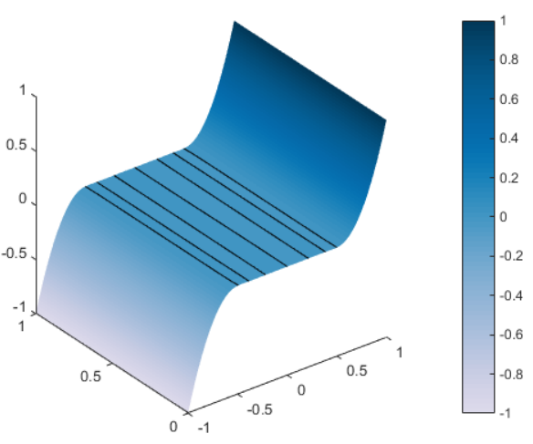
The exact solution is given by the relation independent of ,
| (41) |
and its (exact) energy is The (exact) free boundary is characterized by two lines
The (exact) Lagrange multiplier is then given by
| (42) |
and it is a discontinuous function with a jump on the free boundary. We compute approximation pairs for a sequence of nested uniformly refined meshes. Levels 1 and 2 meshes are depicted in Figure 3. Since some dicretization nodes are lying exactly on the free boundary, there might be a chance to reconstruct the free boundary exactly from approximative solutions. A finer (level 5) approximation pair computed from the dual-based solver is shown in Figure 3. The approximative Lagrange multiplier field however only approximates the exact free boundary. To the given approximation pair , a functional majorant is optimized using 10000 iterations of Algorithm 1 ( we set ). To get more insight on the majorant behaviour, we display space densities of all three additive majorant subparts
separately in Figure 3. The amplitudes of are significantly lower than amplitudes of and , but the value of is still relatively high. The high value of indicates that the exact free boundary is not sufficiently resolved yet and the density of seem to be a reasonable indicator of the exact free boundary.
| level | |||||||
|---|---|---|---|---|---|---|---|
| 1 | 15 | 6.0383 (5.9975) | 7.05e-01 | 1.74e+00 | 1.33e+00 | 3.00e-02 | 3.80e-01 |
| 2 | 45 | 5.5030 (5.5000) | 1.70e-01 | 3.79e-01 | 3.47e-01 | 9.44e-04 | 3.15e-02 |
| 3 | 153 | 5.3765 (5.3750) | 4.32e-02 | 9.14e-02 | 8.41e-02 | 2.47e-05 | 7.28e-03 |
| 4 | 561 | 5.3481 (5.3435) | 1.47e-02 | 2.76e-02 | 2.10e-02 | 6.08e-07 | 6.50e-03 |
| 5 | 2145 | 5.3390 (5.3355) | 5.65e-03 | 8.62e-03 | 5.21e-03 | 7.13e-08 | 3.41e-03 |
Computations on all nested uniformly refined triangular meshes are summarized in 1. The dual energy and primal primal energy converge to the exact energy as . Since we work with nested meshes, we additionally have
The difference of energies is bounded from above by the majorant value as stated in the majorant estimate (26).



Remark 5 (Extension to mixed Dirichlet - Neumann boundary conditions).
This example assumes both Dirichlet and Neumann boundary conditions, but only Dirichlet boundary conditions are considered in . The dual based solver for a double-phase problem can still be applied, with Neumann nodes being added to internal nodes . The majorant estimate (26) is valid with the same majorant form (27), but the flux must satisfy an extra condition on a Neumann boundary, where is a normal vector to the boundary. This condition means that components of from (34) corresponding to Neumann edges must be equal to zero.
4.2 Example II
The second example is also taken from [4] and considers a square domain
| (43) |
constant coefficients
| (44) |
The Dirichlet boundary conditions as assumed in the form
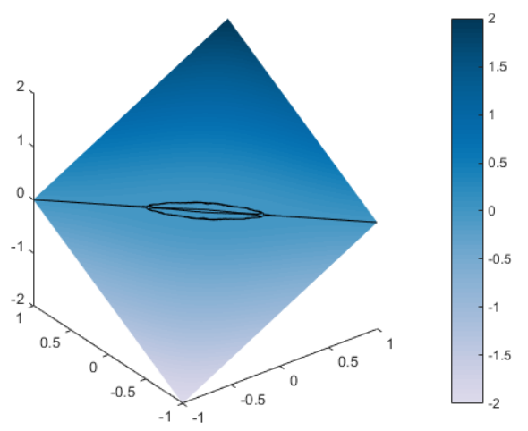
| (45) |
The exact solution is not known for this example. Consequently, no apriori information about the shape of the free boundary or the value of the exact energy is provided. We compute approximation pairs again for a sequence of nested uniformly refined meshes. Levels 1 and 2 meshes are depicted in Figure 7. An approximative solutions pair obtained by the dual-based solver is depicted in Figure 7. The approximative Lagrange multiplier field presumably indicates the exact free boundary. Space distributions of majorant subparts are visualized in Figure 7. We assume that the density of serves as an indicator of the exact free boundary. Table 2 summarizes computations on all nested uniformly refined triangular meshes. The exact energy is not known but it is replaced by the energy of a reference solution in Table 2. The reference solution is computed as on the mesh one level higher (level 6 uniformly refined triangular mesh here).
| level | |||||||
|---|---|---|---|---|---|---|---|
| 1 | 13 | 13.6667 (13.6667) | 6.65e-01 | 2.41e+00 | 2.03e+00 | 3.30e-01 | 5.38e-02 |
| 2 | 41 | 13.1924 (13.1924) | 1.90e-01 | 8.24e-01 | 7.90e-01 | 2.88e-02 | 5.26e-03 |
| 3 | 145 | 13.0491 (13.0489) | 4.71e-02 | 2.18e-01 | 2.15e-01 | 2.20e-03 | 5.24e-04 |
| 4 | 545 | 13.0137 (13.0133) | 1.17e-02 | 5.58e-02 | 5.46e-02 | 1.49e-04 | 1.03e-03 |
| 5 | 2113 | 13.0045 (13.0041) | 2.50e-03 | 1.40e-02 | 1.36e-02 | 1.09e-05 | 4.36e-04 |
| 6 | 8321 | 13.0020 (13.0019) | not evaluated | ||||
Remark 6 (Lower bound of difference of energies based on a reference solution).
If a reference solution is available, its energy satisfies and
| (46) |
The inequality (46) provides actually guaranteed lower and upper bounds of the difference of energies Figure 4 displays convergence of both bounds of for considered 5 levels approximations . By refolmulating (46) we get guranteed bounds of the exact energy
| (47) |
valid for every approximation . For this example, lower bound of create an increasing sequence reported in Table 3.
| level | 1 | 2 | 3 | 4 | 5 |
|---|---|---|---|---|---|
| lower bound of energy | 11.2582 | 12.3686 | 12.8315 | 12.9580 | 12.9905 |



4.3 Implementation details
Both numerical examples are implemented in MATLAB and the code available for download at
http://www.mathworks.com/matlabcentral/fileexchange/57232
The code is based on vetorization techniques of [1, 19]. The main file ’start.m’ is located in the directory ’solver_two_phase_obstacle’. The following parameters can be adjusted:
-
’levels_energy_error’ - the number of the finest uniform triangular level (default is ’5’)
-
’iterations_majorant’ - the number of iterations of Algoritm 2 (default is ’1000’)
The dual based solver of Subsection 3.1 is implemented in ’optimize_energy_dual_mu_constant_compact.m’ and the underlying quadratic programming function ’quadprog’ requires the optimization toolbox of MATLAB to be available. Evalulation of the primal energy for a given function is done in the function ’energy’. This function is able to provide an exact quadrature [14] of the energy for any function , including nondifferentiable terms
5 Conclusions and future outlook
A dual based solution algorithm to provide a finite element approximation of the Lagrange multiplier of the perturbed problem was described and tested on two benchmarks in 2D. The finite elements approximation of the primal minimization problem can be easily reconstructed from Lagrange multipliers by solving one linear system of equations. The quality of such approximation is measured in terms in terms of a fully computational functional majorant. A nonlinear part of the optimized functional majorant seems to work as an indicator of the free boundary. The functional majorant minimization is based on a subsequent minimization and therefore requires many iterations. We would like to speed up majorant optimization in the future.
References
- [1] I. Anjam and J. Valdman: Fast MATLAB assembly of FEM matrices in 2D and 3D: edge elements. Applied Mathematics and Computation 219, 7151–7158, 2013.
- [2] A. Arakelyan : A Finite Difference Method for Two-Phase Parabolic Obstacle-like Problem. Armenian Journal of Mathematics,7,32–49, 2015.
- [3] A. Arakelyan, R. Barkhudaryan, and M. Poghosyan: Numerical solution of the two-phase obstacle problem by finite difference method. Armen. J. Math. 7 (2015), no. 2, 164–182.
- [4] F. Bozorgnia: Numerical solutions of a two-phase membrane problem. Applied Numerical Mathematics, 61, 92–107, 2011.
- [5] H. Buss and S. Repin: A posteriori error estimates for boundary value problems with obstacles. Proceedings of 3nd European Conference on Numerical Mathematics and Advanced Applications, Jÿvaskylä, 1999, World Scientific, 162–170, 2000.
- [6] L. Caffarelli: The obstacle problem revisited. The Journal of Fourier Analysis and Applications, 4, 383–402, 1998.
- [7] Ciarlet P.G., The Finite Element Method for Elliptic Problems. North–Holland, New York, 1978; reprinted as SIAM Classics in Applied Mathematics, Philadelphia, 2002
- [8] I. Ekeland and R. Temam: Convex analysis and variational problems North-Holland, Amsterdam, 1976.
- [9] R. S. Falk: Error estimates for the approximation of a class of variational inequalities. Math. Comput. (1974), 963–971.
- [10] R. Glowinski, J. L. Lions, R. Trémolieres: Numerical analysis of variational inequalities. North-Holland 1981.
- [11] W. Han: A posteriori error analysis via duality theory. Springer 2005.
- [12] P. Harasim, J. Valdman: Verification of functional a posteriori error estimates for obstacle problem in 1D. Kybernetika, 49 (5), 738 – 754, 2013.
- [13] P. Harasim, J. Valdman: Verification of functional a posteriori error estimates for obstacle problem in 2D. Kybernetika, 50 (6), 978 – 1002, 2014.
- [14] J. Kadlec, J. Valdman: Quadrature of the absolute value of a function. MATLAB package. Available at http://www.mathworks.com/matlabcentral/fileexchange/authors/37756.
- [15] D. Kinderlehrer, G. Stampacchia: An Introduction to Variational Inequalities and Their Applications, Academic Press, New York (1980)
- [16] P. Neittaanmäki, S. Repin: Reliable methods for computer simulation (error control and a posteriori estimates). Elsevier, 2004.
- [17] R.H. Nochetto: Sharp -error estimates for semilinear elliptic problems with free boundaries. Numerische Mathematik, 54(3), 243–255, 1989.
- [18] R.H. Nochetto, E. Otárola and A.J. Salgado: Convergence rates for the classical, thin and fractional elliptic obstacle problems. Philos. Trans. A 373 no. 2050, 20140449, 2015.
- [19] T. Rahman and J. Valdman: Fast MATLAB assembly of FEM matrices in 2D and 3D: nodal elements. Applied Mathematics and Computation 219, 7151–7158, 2013.
- [20] S. Repin: A posteriori error estimation for variational problems with uniformly convex functionals. Mathematics of Computation, 69 (230), 481–500, 2000.
- [21] S. Repin: On measures of errors for nonlinear variational problems. Russian Journal of Numerical Analysis and Mathematical Modelling, 6 (27), 577 –- 584, 2012.
- [22] S. Repin and J. Valdman: A posteriori error estimates for two-phase obstacle problem. Journal of Mathematical Sciences 20 (2), 324–336, 2015.
- [23] S. Repin: A posteriori estimates for partial differential equations, Walter de Gruyter, Berlin, 2008.
- [24] H. Shahgholian, N. N. Uraltseva, G. S.Weiss: The Two-Phase Membrane Problem – Regularity of the Free Boundaries in Higher Dimensions, International Mathematics Research Notices, Vol. 2007.
- [25] G. Tran, H. Schaeffer, W. Feldman, and S. Osher: An penalty method for general obstacle problems. SIAM Journal on Applied Mathematics, 75 (4), 1424–1444, 2015.
- [26] N. N. Uraltseva : Two-phase obstacle problem, Journal of Mathematical Sciences, 106 (3), 3073–3077, 2001.
- [27] G. S. Weiss : The Two-Phase Obstacle Problem: Pointwise Regularity of the Solution and an Estimate of the Hausdorff Dimension of the Free Boundary, Interfaces and Free Boundaries, 3 (2), 121–128, 2001.