A Bifurcation Monte Carlo Scheme for Rare Event Simulation

There are many situations where one is interested in an event that happens rarely on the natural time scale of the system [1], [2], [3]. Common examples involve thermal noise assisted transitions from one potential well to another [4]. Direct simulation may be impractical as a way to estimate such transition rates.

There are several approaches to do rare event simulation. Some involve analytic or semi-analytic solution of the associated instanton or large deviations variational problem, e.g., [4]. These methods apply in cases in which a typical rare event trajectory is close to the solution of the variational problem. (Note: “typical” rare event paths are very different from typical paths.) Other methods rely less on theory, and may be preferable in situations where the theory is unavailable or the variational problem is intractable. Some of these, including the bifurcation method presented here, rely on the fact that it is practical to sample the space of typical rare events by Markov chain Monte Carlo (MCMC) even in cases where it is hard to estimate their probability. The bifurcation method presented here is similar to the method of [5], which is applied to problems in queueing theory, and to the method of [6], which is applied to problems of structural reliability. It is similar to the method of nested sampling [7], which, in turn, is motivated by thermodynamic integration.

In the general situation there is a random object, $\mathbf{X}$, with a probability density $f(\mathbf{X})$. We have a function $\phi(\mathbf{X})$. The problem is to estimate

$$p_{\alpha}=\mbox{Pr}\!\left(\phi(\mathbf{X})>\alpha\right)\;.$$

(1)

We are particularly interested in these probabilities when they are very small. In the example presented here, $\mathbf{X}$ represents a path corresponding to some stochastic dynamics, and $\phi(\mathbf{X})$ is a scalar function of the path. The density of the scalar diagnostic variable will be $\rho(\alpha)$, so that

$$\rho(\alpha)\,d\alpha=\mbox{Pr}\!\left(\alpha\leq\phi(\mathbf{X})\leq\alpha+d\alpha\right)\;,$$

and

$$p_{\alpha}=\int_{\alpha}^{\infty}\rho(\alpha^{\prime})\,d\alpha^{\prime}\;.$$

We give a general description of the bifurcation method here with more details for special problems in Sec. 3. At $k=0$, we create $N$ samples $\mathbf{X}^{(0,n)}\sim f$, for $n=1,\ldots,N$, and evaluate the corresponding diagnostic variables,

$$\phi^{(0,n)}=\phi(\mathbf{X}^{(0,n)})\;.$$

These are used to estimate $\alpha_{0}$ as the median of the empirical distribution

$$\widehat{\alpha}_{0}=\mbox{Median}\left\{\phi^{(0,n)}\right\}\;.$$

This $\widehat{\alpha}_{0}$ approximately bifurcates the histogram $\rho(\alpha)$ into the upper and lower $50\%=2^{-1}$ quantiles. In our examples, it is possible to generate independent paths $\mathbf{X}^{(0,n)}$. We call this process as “pre-sampling”.

For any $\alpha$, we define the constrained probability density as

$$f_{\alpha}(\mathbf{X})=\left\{\begin{array}[]{ll}\frac{1}{p_{\alpha}}f(\mathbf{X})&\mbox{ if }\phi(\mathbf{X})>\alpha\\[5.0pt] \;\;0&\mbox{ otherwise.}\end{array}\right.$$

(2)

The constrained histogram density $\rho_{\alpha}$ is similar:

$$\rho_{\alpha}(\alpha^{\prime})=\left\{\begin{array}[]{ll}\frac{1}{p_{\alpha}}\rho(\alpha^{\prime})&\mbox{ if }\alpha^{\prime}>\alpha\\[5.0pt] \;\;0&\mbox{ otherwise.}\end{array}\right.$$

(3)

We assume that it is possible to use MCMC to sample $f_{\alpha}$ starting from a suitably generic $\mathbf{X}$ with $\phi(\mathbf{X})>\alpha$. In the application presented below, we may sample $f_{\alpha}$ using the Crooks-Chandler [8] version of transition path sampling [9], see below.

The bifurcation algorithm is based on the fact that $\alpha_{k}$ is the median of the $\rho_{\alpha_{k-1}}$ histogram. At the start of step $k$, for $k\geq 1$, we have an estimate $\widehat{\alpha}_{k-1}$. We also have a typical sample $\mathbf{X}^{(k,1)}\sim f_{\widehat{\alpha}_{k-1}}$. We run MCMC on the distribution $f_{\widehat{\alpha}_{k-1}}$ to generate enough samples to get a reliable estimate of the median of $\rho_{\widehat{\alpha}_{k-1}}$. This median (the median of the samples as an estimate of the true median) is $\widehat{\alpha}_{k}$. We call this process as “bifurcation loop k”. We also choose at random one of the samples $\mathbf{X}^{(k,n)}$ that has $\phi(\mathbf{X}^{(k,n)})>\widehat{\alpha}_{k}$. This will be $\mathbf{X}^{(k+1,1)}$. Bifurcation loops end when we find the first $k$ with $\widehat{\alpha}_{k}>\alpha$, and let us denote it as $k^{\prime}$. Then we can estimate $p_{\alpha}$ by

$$\widehat{p}_{\alpha}=2^{-k^{\prime}}\times\int_{\alpha}^{\infty}\rho_{\widehat{\alpha}_{k^{\prime}-1}}(\alpha^{\prime})\,d\alpha^{\prime}\;.$$

(4)

The bifurcation method can find rare events more effectively than direct simulation. Suppose $N=10^{7}$ samples are taken at each level. At the end of $k=60$ levels, one is getting samples of events with probability $p_{\alpha_{60}}=2^{-60}\approx 10^{-18}$, having taken only $(k+1)N=6.1\times 10^{8}$ samples in all. This is possible for the following reason: given one typical sample from $f_{\alpha}$, MCMC allows one to get many more, even when $\alpha$ is very small.

We demonstrate in this paper that the bifurcation method can be used to estimate transition rates. We study a system with state $X(t)$ that spends most of its time in stable region $A$ or $B$, with rare transitions between. We first estimate the transition probability $p_{AB}(T)$ for a given time $T$. The random object, $\mathbf{X}$, is the path of $X(t)$ during [0, T]. The transition probability, $p_{AB}(T)$ is estimated by starting the system in region $A$ and estimating the (small) probability that $X_{T}$ is in region $B$, i.e., we define the transition probability as,

$$p_{AB}(T)\equiv\langle h_{B}(X_{T})\rangle\;.$$

(5)

Here, $\langle\cdots\rangle$ denotes a statistical average, and $h_{B}(X_{T})$ is the characteristic function of region B, i.e. $h_{B}(X_{T})=1,$ if $X_{T}$ $\in$ B, else, $h_{B}(X_{T})=0$. If $T$ is taken to be a time longer than the transient time $\tau_{\mbox{\scriptsize ini}}$, but much shorter than the typical time between transitions, $\tau_{\mbox{\scriptsize rxn}}\approx k_{AB}^{-1}$, the transition rate is related to the transition probability by

$$Tk_{AB}\approx p_{AB}(T)\;.$$

(6)

For a practical computation, when $T$ is not very long, it is more accurate to estimate $k_{AB}$ as the plateau value of

$$k_{AB}(t)\equiv\frac{dp_{AB}(t)}{dt}\;.$$

(7)

It can be shown by computational examples that $k_{AB}(t)$ changes during the transient time $\tau_{ini}$. This $\tau_{\mbox{\scriptsize ini}}$ is related to the time needed for the system to reach its local equilibrium in region A. After that, $k_{AB}(t)$ reaches a plateau, and will be a constant for a long time $\tau_{\mbox{\scriptsize rxn}}$. This plateau value is the transition rate $k_{AB}$ in the empirical sense.

This approach does not require a good understanding of the system’s dynamics. It only requires an order parameter $\phi(\mathbf{X})$. It is an advantage of the bifurcation method since it does not require the ”true” (or perfect) reaction coordinate (such as the committor) [9] which is usually quite difficult or impossible to determine in advance for a complex system.

As explained above, we need an MCMC sampler for the constrained distributions $f_{\alpha}$ given by (2). There is a simple way to create one. Choose a Metropolis Hastings sampler for the unconstrained distribution $f$ that has a parameter, $r$, that represents a step size. Small $r$ should correspond to proposals being close to the current sample. Suppose the current sample, $\mathbf{X}^{(n)}$, has the distribution $f_{\alpha}$, and that the proposal is $\mathbf{X}^{(n)}\to\mathbf{Y}$. First perform the usual Metropolis Hastings rejection test on $\mathbf{Y}$. If $\mathbf{Y}$ is accepted in this step, then accept if $\phi(\mathbf{Y})>\alpha$ and set $\mathbf{X}^{(n+1)}=\mathbf{Y}$. Otherwise, if $\phi(\mathbf{Y})<\alpha$, reject and set $\mathbf{X}^{(n+1)}=\mathbf{X}^{(n)}$. It is easy to check that if the original method satisfies detailed balance for $f$, then the modified method satisfies detailed balance for $f_{\alpha}$. If $r$ is small enough and if $\phi(\mathbf{X}^{(n)})>\alpha$, then there is a reasonable probability that $\phi(\mathbf{Y})>\alpha$ also.

Traditional MCMC samplers, such as the Crooks-Chandler method we use, have difficulties in some bifurcation loops due to the fact that paths have fluctuations on many time scales. We propose a multi-scale version of the Crooks-Chandler method that is based on parallel tempering [10] [11] and parallel marginalization [12]. This improves the MCMC efficiency by up to a factor of 38.

In the following sections, we begin with a brief description of the double well problem; then, we describe details of our bifurcation method for this problem, discuss the error estimation of it and methods to improve the efficiency, and describe a method to estimate the transition rate; at last, we show computational results and make a discussion.

The transition rate in a double well potential with small noise is a well studied test problem, which has been used to explore the effectiveness of some rare event sampling methods [13] [14].

Generally, the Langevin dynamics for a noisy system may be written as

$$\frac{dX(t)}{dt}=b(X(t))+\epsilon\dot{W}(t)\;,\qquad X(0)=x_{0}\;,$$

(8)

or in the Itô form

$$dX(t)=b(X(t))dt+\epsilon dW(t)\;,\qquad X(0)=x_{0}\;.$$

(9)

Here, $\dot{W}$ is standard white noise, and $W(t)$ is the corresponding Brownian motion. In a conservative force field, the drift velocity is derived from a potential, $b(X)=-\gamma^{-1}\triangledown U(X)$, where $\gamma$ is the friction coefficient. The parameter $\epsilon=\sqrt{\frac{2k_{B}T}{\gamma}}$, where $k_{B}$ is Boltzmann’s constant and $T$ is the temperature, determines the relative strength of thermal noise and deterministic dynamics. When $U(X)$ has two wells, there are transitions from a locally stable region A to another one B. For small $\epsilon$, the $A\rightarrow B$ transition time is too long to be estimated by direct simulation.

Much theoretical and computational work has gone into this rare-event problem [15] [16] [17] [18]. The theoretical estimate of the transition rate is the Kramers (or Van’t Hoff-Arrhenius) law,

$$k_{AB}=\nu\exp(-\beta E_{a})\;,$$

(10)

where $k_{AB}$ is the transition rate, $\beta=\frac{1}{k_{B}T}$, $E_{a}$ is the activation energy, and $\nu$ is a prefactor. The activation energy is

$$E_{a}=E_{t}-E_{A}\;,$$

(11)

where $E_{A}$ is the energy of region A, and $E_{t}$ is the lowest maximum energy on a path from A to B. We take the specific potential $U(x)=(x^{2}-1)^{2}-1$, which is illustrated in Figure 1. The A and B wells are centered about $x=-1$ and $x=1$ respectively. Their energy is $E_{A}=E_{B}=-1$. The transition energy is $E_{t}=0$. Therefore, the activation energy is $E_{a}=1$.

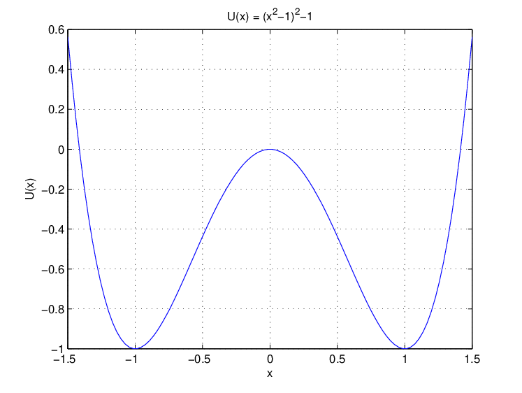
We simulate the stochastic dynamics (8) using the Euler-Maruyama method [19]:

$$\begin{split}X_{t_{i+1}}=X_{t_{i}}+b(X_{t_{i}})\Delta t+\epsilon\sqrt{\Delta t}Z_{i}\;,\\ t_{i}=i\,\Delta t\;,\qquad Z_{i}\sim\mathcal{N}(0,1),\mbox{ (indep)}\;.\end{split}$$

(12)

Here, $\mathcal{N}(0,1)$ is the normal distribution with mean zero and variance one. Figure 2 gives one sample path, calculated for $\epsilon=0.4$, $\gamma=1$, and $\Delta t=10\times 2^{-10}$, which starts from X(0) = -1.

Even with this relatively large noise, transitions are rare and isolated events. A comparable simulation with $\epsilon=0.2$ would show no transitions.

We wish to estimate the transition rate $k_{AB}$ when this rate is very small, using the bifurcation method.

We describe details of the general bifurcation method specific to the transition path problem. The random object is a discrete path, which we denote it as $X_{[0,T]}$,

$$X_{[0,T]}=\{X_{0},\,X_{\Delta t},\,X_{2\Delta t},\,\cdots,X_{T}\}\;.$$

The probability density $f(X_{[0,T]})$ is determined by (12),

$$f(X_{[0,T]})=f(X_{0})\prod_{i=0}^{T/\Delta t-1}p(X_{i\Delta t}\to X_{(i+1)\Delta t})\;,$$

(13)

where $f(X_{0})=\delta(X_{0}-x_{0})$ and

$$p(X_{i\Delta t}\to X_{(i+1)\Delta t})=\frac{1}{\sqrt{2\pi\epsilon^{2}\Delta t}}\exp[-\frac{(X_{(i+1)\Delta t}-X_{i\Delta t}-b(X_{i\Delta t})\Delta t)^{2}}{2\epsilon^{2}\Delta t}]\;.$$

(14)

With this density function, we can find the statistical average of any quantity, for example,

$$\langle h_{B}(X_{T})\rangle=\int f(X_{[0,T]})h_{B}(X_{T})\mathcal{D}X_{[0,T]}\;.$$

(15)

The notation

$$\int\mathcal{D}X_{[0,T]}\equiv\int\prod_{i=0}^{T/\Delta t}dX_{i\Delta t}$$

is borrowed from path integral.

We do pre-sampling by (12), while in bifurcation loops, we use the Crooks-Chandler method to sample the constrained distribution. This method relies on the dynamics (12), which expresses the path $X_{[0,T]}$ in terms of the driving noise

$$Z_{[0,T]}=\{Z_{0},Z_{1},\ldots\}\;.$$

If noise $Z^{(n)}_{[0,T]}$ corresponds to $X^{(n)}_{[0,T]}$, the Crooks-Chandler method generates an independent noise path $\widetilde{Z}_{[0,T]}$ and uses this to create a modified noise path as

$$Z^{\prime}_{[0,T]}=\sqrt{1-r^{2}}\,Z^{(n)}_{[0,T]}+r\widetilde{Z}_{[0,T]}\;.$$

This formula gives $Z^{\prime}_{[0,T]}$ the correct independent ${\cal N}(0,1)$ distribution. The method then calculates $Y_{[0,T]}$, as the corresponding trajectory of (12) with noise $Z^{\prime}_{[0,T]}$. If $Y$ is accepted, then $Z^{(n+1)}_{[0,T]}=Z^{\prime}_{[0,T]}$. Otherwise, $Z^{(n+1)}_{[0,T]}=Z^{(n)}_{[0,T]}$.

Taking the double well potential problem as our computational example, we want to know the transition rate for X changing from well A (near -1) to well B (near 1).

In this paper, we propose a bifurcation method to estimate the transition probability, and apply it to the double well potential problem. In each bifurcation loop, the Crooks-Chandler algorithm is used to do MCMC sampling. We find that during our bifurcation process, some bifurcation loops have very long auto-correlation times when only using the Crooks-Chandler method. When $\epsilon=0.4$ and $\gamma=1$, it happens when we do sampling conditional on $X(10)>\alpha$, where $\alpha\in[-0.5,0.5]$. Sparked by the parallel tempering method and the parallel marginalization method, we propose the “parallel tempering and marginalization” method. With $\epsilon=0.4$ and $\gamma=1$, we take sampling conditional on $X(10)>-0.35$ as a typical example. Our method reduces the time needed to get an almost independent sample from 50,000 units to 1,300 units, while parallel tempering only reduces it to 2750 units. Pointed out by the renormalization theory, judicious elimination of variables by renormalization can reduce long range spatial correlations [22]. So in some other problems, it can reduce the computing time even more. This is another possible advantage to combine the marginalization method together with parallel tempering.

With $\epsilon=0.2$, $\gamma=1$, we test our whole algorithm. By about $7.5\times 10^{8}$ samples, we get the transition probability for $T=5$ is $\widehat{p}(X(5)>0.5)=(5.8\pm 1.8)\times 10^{-22}$. Following that, combining Crooks-Chandler and parallel tempering and marginalization, by one transition path sampling run in the collection of paths which have reached region B in the period [0, 10], with $N=4\times 10^{8}$ samples, we get $\widehat{k}_{AB}\approx(1.7\pm 0.5)\times 10^{-22}$. Analytically, by the Kramers’ theory, the transition rate is

$$k_{AB}=\frac{\omega_{0}\omega_{1}}{2\pi\gamma}\exp(-\frac{2\Delta U}{\gamma\epsilon^{2}})\;,$$

(26)

where $\omega_{0}=\sqrt{\frac{d^{2}U}{dx^{2}}|_{x=-1}}$, $\omega_{1}=\sqrt{-\frac{d^{2}U}{dx^{2}}|_{x=0}}$, and $\Delta U=U(0)-U(-1),$ so $k_{AB,\mbox{\scriptsize Kramer}}=\frac{2\sqrt{2}}{\pi}e^{-\frac{2}{0.04}}=1.7\times 10^{-22}$. For such a small transition rate, we get a pretty good estimation of the transition rate within affordable computational time by our bifurcation method.

At last, we would like to mention that the bifurcation method can be generalized. In the bifurcation loop $k$, we can set $\alpha_{k}$ to satisfy the following equation,

$$\mbox{Pr}_{\alpha_{k-1}}(\phi(X_{[0,T]})\geq\alpha_{k})\equiv\int_{\phi(X_{[0,T]})\geq\alpha_{k}}f_{\alpha_{k-1}}(X_{[0,T]})\mathcal{D}X_{[0,T]}=c\;,$$

(27)

where $0<c<1$. If c is 0.5, it is our bifurcation method proposed in this paper.

References

- [1] K. Fichthorn, E. Gulari, R. Ziff, “Noise-induced Bistability in a Monte Carlo Surface-Reaction Model”, Phys. Rev. Lett. 63, 1527, Oct. 1989.
- [2] S. Kadar, J. Wang, K. Showalter, “Noise-supported traveling waves in sub-excitable media”, Nature, Vol. 391, Feb. 1998.
- [3] J. N. Onuchic, Z. Luthey-Schulten, P. G. Wolynes, “Theory of protein folding: the energy landscape perspective”, Annual Review of Physical Chemistry Vol. 48, Pages 545–600, Oct. 1997.
- [4] K. Martens, D. L. Stein, and A. D. Kent, “Thermally Induced Magnetic Switching in Thin Ferromagnetic Annuli”, Proc. SPIE 5845, June 2005.
- [5] Sungjae Jun, PhD thesis, NYU, 2013.
- [6] K. Zuev, “Subset Simulation Method for Rare Event Estimation: An Introduction”, https://arxiv.org/abs/1505.03506, 2015.
- [7] John Skilling, “Nested Sampling”, AIP Conference Proceedings 735: 395–-405, 2004.
- [8] G. E. Crooks and D. Chandler, “Efficient transition path sampling for non-equilibrium stochastic dynamics”, Phys. Rev. E, 64, 026109, 2001.
- [9] C. Dellago, P. G. Bolhuis, P. L. Geissler, “Transition Path Sampling”, Advances in Chemical Physics, Oct. 2001.
- [10] R. H. Swendsen and J. Wang, “Replica Monte Carlo Simulation of Spin Glasses”, Physical Review Letters, Volume 57, Pages 2607–2609, 1986.
- [11] K. Hukushima, and K. Nemoto, “Exchange Monte Carlo Method and Application to Spin Glass Simulations”, J. Phys. Soc. Jpn. 65, 1604, 1996.
- [12] J. Weare, “Efficient Monte Carlo sampling by parallel marginalization”, PNAS, Pages 12657–12662, July 2007.
- [13] Weinan E, Weiqing Ren, Eric Vanden-Eijnden, “String method for the study of rare events”, Physical Review B 66, 052301, 2002.
- [14] Eric Vanden-Eijnden, Jonathan Weare, “Rare Event Simulation of Small Noise Diffusions”, Communications on Pure and Applied Mathematics, Vol. 65, Issue 12, 2012.
- [15] P. Hnggi, P. Talkner, M. Borkovec, “Reaction-rate theory: fifty years after Kramers”, Review of Modern Physics, Vol. 62, No.2, April 1990.
- [16] H. A. Kramers, “Brownian Motion in a Field of Force and the Diffusion Model of Chemical Reactions”, Physica, Volume 7, Issue 4, Pages 284–304, April 1940.
- [17] L. Gong, D. L. Stein, “The Escape Problem in a Classical Field Theory With Two Coupled Fields”, Journal of Physics A: Mathematical and Theoretical 43 (40), 405004, 2010.
- [18] L. Gong, D. L. Stein, “Noisy classical field theories with two coupled fields: Dependence of escape rates on relative field stiffness”,Physical Review E 84 (3), 031119, 2011.
- [19] P. E. Kloeden, and E. Platen, “Numerical Solution of Stochastic Differential Equations”, Springer, Berlin, 1992.
- [20] A. D. Sokal, “Monte Carlo Methods in Statistical Mechanics: Foundations and New Algorithms”
- [21] J. Goodman, http://www.math.nyu.edu/faculty/goodman/software/acor
- [22] J. Binney, N. Dowrick, A. Fisher, M. Newman, “The theory of Critical Phenomena: An Introduction to the Renormalization Group”, Oxford University Press, New York, 1992.