跳到论文正文
W Papers独立论文阅读器 arXiv:1606.00105 论文正文 计算阅读时间 · 0%
引用这篇论文根据当前论文元数据生成,正式投稿前建议核对。


License: arXiv.org perpetual non-exclusive license
arXiv:1606.00105v1 [nucl-th] 01 Jun 2016

Quantum corrections to the Relativistic Mean-Field theory

Sergei P. Maydanyuk(1,2) Email: maidan@kinr.kiev.ua Affiliation: (1)(1)Institute of Modern Physics, Chinese Academy of Sciences, Lanzhou, 730000, China    Peng-Ming Zhang1 Email: zhpm@impcas.ac.cn Affiliation: (1)(1)Institute of Modern Physics, Chinese Academy of Sciences, Lanzhou, 730000, China    Ahmed Bakry1 Email: abakry@impcas.ac.cn Affiliation: (1)(1)Institute of Modern Physics, Chinese Academy of Sciences, Lanzhou, 730000, China Affiliation: (2)(2)Institute for Nuclear Research, National Academy of Sciences of Ukraine, Kiev, 03680, Ukraine
August 24, 2026
Abstract

In this paper, we have compared the RMF theory and the model of deformed oscillator shells (DOS) in description of the quantum properties of the bound states of the spherically symmetric light nuclei. We have obtained an explicit analytical relation between differential equations for the RMF theory and DOS model, which determine wave functions for nucleons. On such a basis we perform analysis of correspondence of quantum properties of nuclei. Conclusions are the following. (1) On the basis of the relations above, we found the potential VR​M​FV_{RMF} of the RMF theory for nucleons which has the wave functions ff and gg for nucleons with joint part hh coincident exactly analytically with the nucleon wave function of DOS model with potential VshellV_{\rm shell}. This fact confirms that it is possible to describe quantum properties of nucleus in framework of the RMF theory exactly the same as in DOS model. However, a difference between VR​M​FV_{RMF} and VshellV_{\rm shell} is essential for any nucleus. (2) The nucleon wave functions and densities obtained by the DOS and RMF theories are essentially different. The nucleon densities of the RMF theory contradict to knowledge about distribution of the proton and neutron densities inside the nuclei obtained from experimental data. This indicates that gg and ff have no sense of the wave functions of quantum physics. But, hh provides proper description of quantum properties of nucleons inside the nucleus. (3) We calculate meson function w0w^{0} (and corresponding potential VwV_{w} in framework of RMF theory) based on the found nucleon density above. (4) ff and gg are not solutions of Dirac equation with VwV_{w}. If the meson theory describes quantum properties of nucleus well, then a difference between VwV_{w} and VR​M​FV_{RMF} should be as small as possible. We introduce new quantum corrections characterizing difference between these potentials. We find that (a) The function w0w^{0} should be reinforced strongly, (b) The corrections are necessary to describe the quantum properties of the nuclei.

Keywords: 
Relativistic mean-field theory, effective Lagrangian, Shell model, Resonating group approach, many-nucleon system, quantum mechanics, ground state properties of finite nuclei, bound state, tunneling
pacs
21.60.Jz, 21.60.Cs, 03.65.Xp 21.10.Gv, 21.65.Jk, 21.10.Ft

I Introduction

Nuclear interactions are one of the most fundamental subject in physics, which attracted scientists for a very long time and a lot of efforts were put to their understanding. Here, many theories have been developed. In this paper we put our interest to two different theories.

The first one is the Relativistic mean-field (RMF) theory (see Refs. [1, 2, 3, 4, 5, 6, 7, 8, 9] and reference therein) which is based on the relativistic formulation of unified lagrangian, combining nucleons of the studied nuclear system, while nuclear interactions are described via exchange of mesons of different types. This theory, initially born in the 1970s from works of John Dirk Walecka on quantum hadrodynamics, from end of 1980s has been intensively investigated by Piter Ring and coworkers and then many other researchers. It seems this theory is one of the most actively developed and successful in nuclear physics, as it now well describes all known properties of nuclear structure (for example, see general properties [12, 13, 11, 10], deformations and asymmetries [14, 15], superdeformations [12, 16, 17, 18], magnetic multipole moments and transition probabilities [19], magnetic rotation bands [20], collective rotational motion in deformed nuclei [21], shell structure [22], pseudospin symmetry for bound states [23], anomaly in the charge radii [24], phase transitions in nuclear matter [25], etc.), is applied for analysis of nuclear reactions (for example, see for fission [26, 27, 28, 29]), is used in different tasks of nuclear astrophysics [30, 31, 32, 33], exotic nuclei [34, 9], hypernuclei [35], etc. In frameworks of such a theory, nucleons obey the Dirac equation, while the mesons obey the Klein-Gordon equations (i.e. equations of motion). Essential efforts are put to understanding of nuclear matter, symmetry energy and binding energy of nuclei in the region from the lightest to heavy, and even superheavy [36, 37].

The second theory is a microscopic nuclear theory of nucleus (MN theory) which is unified theory oriented on the fully quantum basis in description of properties of the nuclear structure, scattering and reactions [38, 39, 40]. It is very effective in detailed study and description of clustering phenomena in nuclei. The resultant formalism is now generally known as the Generator coordinate method [41, 42, 43] introduced by Hill, Griffin and Wheeler [44, 45]. However, it should be mentioned, that this method is equivalent to the Resonating group method [39] proposed by Wheeler in Refs. [46, 47]. Since 1970-s, a model of the deformed oscillator shells (DOS) as a part of this theory was successfully developed for study of bound states of nuclear systems [48] (note an Algebraic model of the resonating group method [49, 50, 51, 52, 53, 54, 55] which is a unified approach to describe bound and continuous states of nuclear systems, a microscopic continuum-discretized coupled-channels reaction approach [56, 57, 58] oriented on the microscopic description of reactions, see also reference therein). Such a model represents the nuclear many-particle wave functions through their expansions in harmonic oscillator eigenstates (with application of Pauli principle), where nucleon-nucleon potentials are parameterized from data of the experimental nucleon-nucleon scattering. In frameworks of such a model, the light nuclei starting from He4{}^{4}{\rm He} were investigated, with a good agreement with known experimental information for them. This model clearly well describes physics of the light nuclei (binding energy, sizes, deformations, quadruple momenta, etc.) and, so, we shall focus on it in study of bound states of these nuclei in this paper. It is important that this model forms a clear accurate quantum basis for more complicated unified microscopic nuclear theory in description of bound states of the light nuclei.

At a brief comparison of these two theories one can find, that wave function of nucleons in the RMF theory is solution of Dirac equation (with interacting meson potential), while a corresponding nucleon wave function in the MN theory is solution of the Schrödinger equation. This fact provides a principal difference between properties and behavior of these wave functions of two theories: these two wave functions are never identical at any arbitrary interacting potentials, in principle.11 1 We prove this statement by Eqs. (37), see below in the text. Exception is for free particle moving in vacuum only. By such a reason, one can suppose that this difference should be shown both in different description of nuclear structure (bound states), and moreover in nuclear reactions (unbound states, i.e. scattering, decay, capture states, etc.). In particular, it becomes clear from such a logic that nucleon densities in nuclei are always different in framework of two theories. As the wave function is key characteristic of quantum properties of the studied object in quantum mechanics, one can conclude that these two theories cannot provide the same quantum description of the nuclei and nuclear reactions.22 2 One can remind that Dirac equation was written for description of free point-like fermion in vacuum in order to include relativistic relations between space and time, while the Schrödinger equation was devote to the most accurate description of the quantum properties of the studied (spinless) system (which can be complicated) in the interacting potential.

So, a main aim of this paper is to clarify and resolve this puzzle. We analyze and compare these two theories in their quantum description of the nuclear properties and interactions. In order to find key idea and analyze it as clearly as possible, we choose the light nucleus He4{}^{4}{\rm He} for our analysis and calculations. As this nucleus is spherically symmetric, we can apply the spherically symmetric approximation that reduces essentially number of equations. It turns out that one can find an explicit analytical relation between differential equations for the RMF theory and DOS model, which determine wave functions for nucleons. These relation is powerful tools for performing a comparative quantum analysis of these two theories. As a mathematical basis of the RMF theory for analysis in this paper, we use equations of motions as Eqs. (36)–(40) in Ref. [2], densities as Eqs. (41)–(44) in Ref. [2], potentials as Eqs. (45)–(46) in Ref. [2].

This paper is organized by the following. In Sec. II and III we obtain an explicit analytical relation between differential equations for the RMF theory and DOS model, which determine wave functions for nucleons. Here, we present a new approach for determination of a transformed new potential and part of the Dirac wave function corresponding to the potential and wave function of the shell model. A comparative analysis of the potential of the RMF theory found by such a way with a corresponding potential of the shell model is given in Sec. IV. We start practical calculations and analysis on the example of the He4{}^{4}{\rm He} nucleus, which is used in demonstrations of all next found characteristics. The wave function and corresponding density for nucleons are defined and calculated in Sec. V. Here, we add an series expansion approach for determination of these characteristics, which is effective in next determination of the meson potential and quantum corrections. The meson potential based on the nucleon density found above is obtained in Sec. VI, the quantum corrections are defined and calculated in Sec. VII. In Sec. VIII we summarize the paper. Some needed details of calculations are added in Appendixes A– D.

II Spherically symmetric consideration

We start from equation of motion of the RMF theory for nucleon with number ii defined in Eq. (36) in Ref. [2] (in this section we remove the index of numeration of nucleons):

{−iα∇+β(m0+S(𝐫))+V(𝐫))}ψ(𝐫)=εψ(𝐫),\begin{array}[]{lcl}\bigl\{-i\,\alpha\nabla\,+\beta\,(m_{0}+S(\mathbf{r}))+V(\mathbf{r}))\bigr\}\,\psi(\mathbf{r})=\varepsilon\,\psi(\mathbf{r}),\\ \end{array} (1)

where mm is mass of nucleon, V⁡(𝐫)V(\mathbf{r}) and S⁡(𝐫)S(\mathbf{r}) are potentials defined in Eqs. (45) and (46) in Ref. [2]. If V⁡(r)V(r) and S⁡(r)S(r) are radial functions, we look for a solution for wave function in form (see Sect. 1.5.1, page 48 in Ref. [60]):

ψε​j​l​M​(𝐫)=(φε​j​l​M​(𝐫)χε​j​l​M​(𝐫)),\begin{array}[]{lcl}\psi_{\varepsilon jlM}(\mathbf{r})=\left(\begin{array}[]{lcl}\varphi_{\varepsilon jlM}(\mathbf{r})\\ \chi_{\varepsilon jlM}(\mathbf{r})\end{array}\right),\end{array} (2)

where

φε​j​l​M​(𝐫)=g⁡(r)​Ωj​l​M​(𝐧),χε​j​l​M​(𝐫)=i​f​(r)​Ωj​l′​M​(𝐧),\begin{array}[]{lcl}\varphi_{\varepsilon jlM}(\mathbf{r})=g\,(r)\;\Omega_{jlM}(\mathbf{n}),&\chi_{\varepsilon jlM}(\mathbf{r})=i\,f\,(r)\;\Omega_{jl^{\prime}M}(\mathbf{n}),\end{array} (3)

and Ωj​l​M​(𝐧)\Omega_{jlM}(\mathbf{n}) is spherical harmonic spinor (called also as spherical harmonic spinor function), l′=2​j−ll^{\prime}=2j-l, 𝐧=𝐫/r\mathbf{n}=\mathbf{r}/r, r=|𝐫|r=|\mathbf{r}|, g⁡(r)g\,(r) and f⁡(r)f\,(r) are radial functions. According to Ref. [60], ε\varepsilon is eigenvalue for Hamiltonian (but it is not energy for particle), which can be positive and negative. At ε>0\varepsilon>0 equations describe particle, at ε<0\varepsilon<0 — antiparticle. Energy is defined as E=|ε|E=|\varepsilon|, i. e. it is positive for particles and antiparticles.

In the case when scalar potential S⁡(r)=S0S(r)=S_{0} is constant, Eq. (1) can be transformed explicitly to the differential equation of the second order (Schrödinger type equation) as (see Appendix A):

−h′′+V¯​(r)​h=0,-\,h^{\prime\prime}+\bar{V}(r)\,h=0, (4)

where h⁡(r)h(r) is a new unknown wave function and a new potential is introduced as

V¯​(r)=V′′2​(ε+m−V)+3​(V′)24​(ε+m−V)2−V′ε+m−V⁡(r)​χr−[ε−V⁡(r)]2+m2+χ⁡(1+χ)r2,\begin{array}[]{cc}\bar{V}(r)=\displaystyle\frac{V^{\prime\prime}}{2\,(\varepsilon+m-V)}+\displaystyle\frac{3\,(V^{\prime})^{2}}{4\,(\varepsilon+m-V)^{2}}-\displaystyle\frac{V^{\prime}}{\varepsilon+m-V(r)}\,\displaystyle\frac{\chi}{r}\,-\bigl[\varepsilon-V(r)\bigr]^{2}+m^{2}+\displaystyle\frac{\chi(1+\chi)}{r^{2}},\end{array} (5)

and m=m0+S0m=m_{0}+S_{0}, χ=l⁡(l+1)−j⁡(j+1)−1/4\chi=l(l+1)-j(j+1)-1/4 (see (1.4.6), page 44 in [60]). The unknown new wave function h⁡(r)h(r) and its derivative h′​(r)h^{\prime}(r) should be obtained via numeric solution of Eq. (4) with the potential V¯​(r)\bar{V}(r). Then, the old wave function is obtained as (see Appendix A)

g⁡(r)=n0​|ε+m−V⁡(r)|r⋅h⁡(r),f⁡(r)=sign⁡[ε+m−V⁡(r)]​n0r​|ε+m−V⁡(r)|​{[−V′​(r)2​(ε+m−V​(r))+χr]​h​(r)+h′​(r)},\begin{array}[]{lcl}g\,(r)&=&\displaystyle\frac{n_{0}\;\sqrt{|\varepsilon+m-V(r)|}}{r}\cdot h\,(r),\\ f\,(r)&=&{\rm sign}\,\bigl[\varepsilon+m-V(r)\bigr]\;\displaystyle\frac{n_{0}}{r\>\sqrt{|\varepsilon+m-V(r)|}}\;\biggl\{\Bigl[\displaystyle\frac{-V^{\prime}(r)}{2\>(\varepsilon+m-V(r))}+\displaystyle\frac{\chi}{r}\;\Bigr]\;h\,(r)+h^{\prime}\,(r)\biggr\},\end{array} (6)

where n0n_{0} is free arbitrary constant and

sign⁡[x]={1,at ​x>0,−1,at ​x<0.{\rm sign}\,\bigl[x\bigr]=\left\{\begin{array}[]{ll}1,&\mbox{\rm at }x>0,\\ -1,&\mbox{\rm at }x<0.\end{array}\right. (7)

Also we have a property sign⁡[−x]=−sign⁡[x]{\rm sign}\,\bigl[-x\bigr]=-\,{\rm sign}\,\bigl[x\bigr].

We rewrite the solutions above via dimensionless variable. In this connection, it is convenient to introduce, instead of the coordinate rr, a new dimensionless variable ξr\xi_{r} by the relation

ξr=rar,\xi_{r}=\displaystyle\frac{r}{a_{r}}, (8)

where ara_{r} is a new coefficient defined from the shell model for the chosen studied nucleus. After transformations Eq. (4) is transformed to

−d2​hd​ξr2+V¯ξ​(ξr)​h=0,-\,\displaystyle\frac{d^{2}h}{d\xi_{r}^{2}}+\bar{V}_{\xi}(\xi_{r})\,h=0, (9)

where

V¯ξ​(ξr)=V′′2​(ε+m−V)+3​(V′)24​(ε+m−V)2−V′ε+m−V​χξr−ar2​[ε−V]2+ar2​m2+χ⁡(1+χ)ξr2,\begin{array}[]{cc}\bar{V}_{\xi}(\xi_{r})=\displaystyle\frac{V^{\prime\prime}}{2\,(\varepsilon+m-V)}+\displaystyle\frac{3\,(V^{\prime})^{2}}{4\,(\varepsilon+m-V)^{2}}-\displaystyle\frac{V^{\prime}}{\varepsilon+m-V}\,\displaystyle\frac{\chi}{\xi_{r}}-a_{r}^{2}\bigl[\varepsilon-V\bigr]^{2}+a_{r}^{2}m^{2}+\displaystyle\frac{\chi(1+\chi)}{\xi_{r}^{2}},\end{array} (10)

the wave radial functions g⁡(ξr)g(\xi_{r}) and f⁡(ξr)f(\xi_{r}) have the following solutions:

g⁡(ξr)=nξ​0​|ε+m−V⁡(ξr)|ξr⋅h⁡(ξr),f⁡(ξr)=sign⁡[ε+m−V⁡(ξr)]​nξ​0ar​ξr​|ε+m−V⁡(ξξr)|​{[−V′​(ξr)2​(ε+m−V⁡(ξr))+χξr]​h​(ξr)+h′​(ξr)}\begin{array}[]{lc}g\,(\xi_{r})=\displaystyle\frac{n_{\xi 0}\;\sqrt{|\varepsilon+m-V(\xi_{r})|}}{\xi_{r}}\cdot h\,(\xi_{r}),\\ f\,(\xi_{r})={\rm sign}\,\bigl[\varepsilon+m-V(\xi_{r})\bigr]\;\displaystyle\frac{n_{\xi 0}}{a_{r}\xi_{r}\>\sqrt{|\varepsilon+m-V(\xi_{\xi_{r}})|}}\;\biggl\{\Bigl[\displaystyle\frac{-V^{\prime}(\xi_{r})}{2\>(\varepsilon+m-V(\xi_{r}))}+\displaystyle\frac{\chi}{\xi_{r}}\;\Bigr]\;h\,(\xi_{r})+h^{\prime}\,(\xi_{r})\biggr\}\end{array} (11)

and nξ​0n_{\xi 0} is a new arbitrary constant of integration.

III Determination of potential VV on the basis of the given V¯\bar{V}

We shall rewrite the unknown potential V⁡(r)V(r) on the basis of the known potential V¯​(r)\bar{V}(r). We introduce the following change of potential:

V1​(r)=V⁡(r)−ε−mV_{1}(r)=V(r)-\varepsilon-m (12)

and from Eq. (5) we obtain

V¯​(r)=−V1′′2​V1+3​(V1′)24​V12+V1′V1​χr−[V1+m]2+m2+χ⁡(1+χ)r2.\begin{array}[]{cc}\bar{V}(r)=-\,\displaystyle\frac{V_{1}^{\prime\prime}}{2\,V_{1}}+\displaystyle\frac{3\,(V_{1}^{\prime})^{2}}{4\,V_{1}^{2}}+\displaystyle\frac{V_{1}^{\prime}}{V_{1}}\,\displaystyle\frac{\chi}{r}\,-\bigl[V_{1}+m\bigr]^{2}+m^{2}+\displaystyle\frac{\chi(1+\chi)}{r^{2}}.\end{array} (13)

In case of the spherically symmetric nuclei in the ground state we have:

l=0,j=12,χ=−1\begin{array}[]{ccc}l=0,&j=\displaystyle\frac{1}{2},&\chi=-1\end{array} (14)

and

4​V¯​(r)​V12=−2​V1​V1′′+3​(V1′)2−4r​V1​V1′−4​V14−8​V13​m.\begin{array}[]{cc}4\,\bar{V}(r)V_{1}^{2}=-2\,V_{1}V_{1}^{\prime\prime}+3\,(V_{1}^{\prime})^{2}-\displaystyle\frac{4}{r}\,V_{1}V_{1}^{\prime}\,-4\,V_{1}^{4}-8\,V_{1}^{3}\,m.\end{array} (15)

The next task is to find the unknown V1V_{1} on the basis of the given V¯\bar{V}.

III.1 Solutions in form of series

We shall analyze a possibility of existence of solution of equation (15) in form of series:

V1​(r)=f0+∑n=1Nfn​rn,V1′​(r)=f1+∑n=1(n+1)​fn+1​rn,V1′′​(r)=2​f2+∑n=1(n+1)​(n+2)​fn+2​rn.\begin{array}[]{lcl}\vskip 2.84526ptV_{1}(r)&=&f_{0}+\displaystyle\sum\limits_{n=1}^{N}f_{n}r^{n},\\ \vskip 2.84526ptV_{1}^{\prime}(r)&=&f_{1}+\displaystyle\sum\limits_{n=1}(n+1)f_{n+1}r^{n},\\ V_{1}^{\prime\prime}(r)&=&2f_{2}+\displaystyle\sum\limits_{n=1}(n+1)(n+2)f_{n+2}r^{n}.\end{array} (16)

We consider potential in the following form:

V¯​(r)=a0+a1​r+a2​r2,\bar{V}(r)=a_{0}+a_{1}r+a_{2}r^{2}, (17)

where a0a_{0}, a1a_{1} and a3a_{3} are parameters, defined by the microscopic shell model of nucleus. Taking into account the initial equation (15), we obtain equation for determination of the unknown amplitudes fnf_{n}. Solving this equation (see App. B, for details), we obtain such amplitudes (at n≥2n\geq 2, also we shall use f−1=f−2=0f_{-1}=f_{-2}=0):

f1=0,f2=−f03​[a0+2​m​f0+f02],f3=−a1​f03,fn+2=−f2​fn(n+2)​f0+1(n+2)​f0∑s=0n[(s+1)​(3​n−5​s−1)4fs+1fn−s+1−−fs(a0fn−s+a1fn−s−1+a2fn−s−2)−∑p=0s∑t=0pftfp−tfs−pfn−s−2m∑t=0sftfs−tfn−s].\begin{array}[]{lcl}\vskip 4.2679ptf_{1}&=&0,\\ \vskip 4.2679ptf_{2}&=&-\displaystyle\frac{f_{0}}{3}\,\bigl[a_{0}+2mf_{0}+f_{0}^{2}\bigr],\\ \vskip 4.2679ptf_{3}&=&-\,\displaystyle\frac{a_{1}f_{0}}{3},\\ \vskip 1.42262ptf_{n+2}&=&-\,\displaystyle\frac{f_{2}f_{n}}{(n+2)\,f_{0}}\>+\>\displaystyle\frac{1}{(n+2)\,f_{0}}\,\displaystyle\sum\limits_{s=0}^{n}\Bigl[\displaystyle\frac{(s+1)\,(3n-5s-1)}{4}\,f_{s+1}\,f_{n-s+1}\;-\\ &-&f_{s}\,\bigl(a_{0}f_{n-s}+a_{1}f_{n-s-1}+a_{2}f_{n-s-2}\bigr)-\displaystyle\sum\limits_{p=0}^{s}\displaystyle\sum\limits_{t=0}^{p}f_{t}\,f_{p-t}\,f_{s-p}\,f_{n-s}-2m\displaystyle\sum\limits_{t=0}^{s}f_{t}f_{s-t}\,f_{n-s}\Bigr].\end{array} (18)

Note that there is arbitrary choice in definition for f0f_{0} (our analysis has shown that variations of this coefficient change strongly the potential V1V_{1} for larger rr). So, for it definition, it needs to introduce a new additional condition (see further in text).

III.2 Representation of solutions via dimensionless variable

In dimensionless variable (8), for the spherically symmetric nuclei in the ground state we have the following change of potential

V1​(ξr)=V⁡(ξr)−ε−mV_{1}(\xi_{r})=V(\xi_{r})-\varepsilon-m (19)

and Eq. (15) is transformed into

4​V¯ξ​(ξr)​V12=−2​V1​V1′′+3​(V1′)2−4ξr​V1​V1′−4​ar2​V14−8​ar2​V13​m.\begin{array}[]{cc}4\,\bar{V}_{\xi}(\xi_{r})V_{1}^{2}=-2\,V_{1}V_{1}^{\prime\prime}+3\,(V_{1}^{\prime})^{2}-\displaystyle\frac{4}{\xi_{r}}\,V_{1}V_{1}^{\prime}\,-4\,a_{r}^{2}V_{1}^{4}-8\,a_{r}^{2}V_{1}^{3}\,m.\end{array} (20)

Solution of this equation in the dimensionless variable ξr\xi_{r} obtains form:

V1​(ξr)=∑n=0fξ,n​ξrn,V1′​(ξr)=∑n=0(n+1)​fξ,n+1​ξrn,V1′′​(ξr)=∑n=0(n+1)​(n+2)​fξ,n+2​ξrn,\begin{array}[]{lcl}\vskip 2.84526ptV_{1}(\xi_{r})&=&\displaystyle\sum\limits_{n=0}f_{\xi,n}\xi_{r}^{n},\\ \vskip 2.84526ptV_{1}^{\prime}(\xi_{r})&=&\displaystyle\sum\limits_{n=0}(n+1)f_{\xi,n+1}\xi_{r}^{n},\\ V_{1}^{\prime\prime}(\xi_{r})&=&\displaystyle\sum\limits_{n=0}(n+1)(n+2)f_{\xi,n+2}\xi_{r}^{n},\end{array} (21)

where (n≥2n\geq 2, we use fξ,−1=fξ,−2=0f_{\xi,-1}=f_{\xi,-2}=0)

fξ,1=0,fξ,2=−fξ,03​[aξ,0+2​ar2​m​fξ,0+ar2​fξ,02],fξ,3=−aξ,1​fξ,03,fn+2=−f2​fn(n+2)​f0+1(n+2)​f0∑s=0n[(s+1)​(3​n−5​s−1)4fs+1fn−s+1−−ar2∑p=0s∑t=0pftfp−tfs−pfn−s−2ar2m∑t=0sftfs−tfn−s−fs(aξ,0fn−s+aξ,1fn−s−1+aξ,2fn−s−2)]\begin{array}[]{lcl}\vskip 4.2679ptf_{\xi,1}&=&0,\\ \vskip 4.2679ptf_{\xi,2}&=&-\displaystyle\frac{f_{\xi,0}}{3}\,\bigl[a_{\xi,0}+2a_{r}^{2}mf_{\xi,0}+a_{r}^{2}f_{\xi,0}^{2}\bigr],\\ \vskip 4.2679ptf_{\xi,3}&=&-\,\displaystyle\frac{a_{\xi,1}f_{\xi,0}}{3},\\ \vskip 1.42262ptf_{n+2}&=&-\,\displaystyle\frac{f_{2}f_{n}}{(n+2)\,f_{0}}\>+\>\displaystyle\frac{1}{(n+2)\,f_{0}}\,\displaystyle\sum\limits_{s=0}^{n}\Bigl[\displaystyle\frac{(s+1)\,(3n-5s-1)}{4}\,f_{s+1}\,f_{n-s+1}\;-\\ &-&a_{r}^{2}\displaystyle\sum\limits_{p=0}^{s}\displaystyle\sum\limits_{t=0}^{p}f_{t}\,f_{p-t}\,f_{s-p}\,f_{n-s}-2a_{r}^{2}m\displaystyle\sum\limits_{t=0}^{s}f_{t}f_{s-t}\,f_{n-s}-f_{s}\,\bigl(a_{\xi,0}f_{n-s}+a_{\xi,1}f_{n-s-1}+a_{\xi,2}f_{n-s-2}\bigr)\Bigr]\end{array} (22)

and we use the potential V¯ξ\bar{V}_{\xi} in a form

V¯ξ​(ξ)=aξ,0+aξ,1​ξr+aξ,2​ξr2,\bar{V}_{\xi}(\xi)=a_{\xi,0}+a_{\xi,1}\xi_{r}+a_{\xi,2}\xi_{r}^{2}, (23)

where aξ,0a_{\xi,0}, aξ,1a_{\xi,1} and aξ,2a_{\xi,2} are parameters, defined by the microscopic shell model of nucleus, fξ,0f_{\xi,0} is arbitrary.

III.3 Approach of Numerov’s type for solution

We develop discrete solution approach to find the unknown potential. At point ξr,n\xi_{r,n} we have v1,n=V1​(ξr,n)v_{1,n}=V_{1}(\xi_{r,n}) and write derivatives:

V1′​(ξr,n)=v1,n′=v1,n−v1,n−1Δ,V1′′​(ξr,n)=v1,n′′=v1,n+1−2​v1,n+v1,n−1Δ2.\begin{array}[]{cc}V_{1}^{\prime}(\xi_{r,n})=v_{1,n}^{\prime}=\displaystyle\frac{v_{1,n}-v_{1,n-1}}{\Delta},&V_{1}^{\prime\prime}(\xi_{r,n})=v_{1,n}^{\prime\prime}=\displaystyle\frac{v_{1,n+1}-2v_{1,n}+v_{1,n-1}}{\Delta^{2}}.\end{array} (24)

We rewrite Eq. (20) as

4​v¯ξ,n​v1,n2=−2​v1,n​v1,n+1−2​v1,n+v1,n−1Δ2+3​(v1,n−v1,n−1Δ)2−4ξr​v1,n​(v1,n−v1,n−1Δ)−4​ar2​v1,n4−8​ar2​v1,n3​m.\begin{array}[]{cc}4\,\bar{v}_{\xi,n}v_{1,n}^{2}=-2\,v_{1,n}\displaystyle\frac{v_{1,n+1}-2v_{1,n}+v_{1,n-1}}{\Delta^{2}}+3\,\Bigl(\displaystyle\frac{v_{1,n}-v_{1,n-1}}{\Delta}\Bigr)^{2}-\displaystyle\frac{4}{\xi_{r}}\,v_{1,n}\Bigl(\displaystyle\frac{v_{1,n}-v_{1,n-1}}{\Delta}\Bigr)\,-4\,a_{r}^{2}v_{1,n}^{4}-8\,a_{r}^{2}v_{1,n}^{3}\,m.\end{array} (25)

Solving this equation, we obtain:

v1,n+1=2​Δ2​v¯ξ,n​v1,n+72​v1,n−4​v1,n−1+32​v1,n​v1,n−12−2​Δ​v1,nξr,n+2​Δ​v1,n−1ξr,n−2​Δ2​ar2​v1,n3−4​Δ2​ar2​v1,n2​m.\begin{array}[]{ccl}v_{1,n+1}&=&2\,\Delta^{2}\,\bar{v}_{\xi,n}v_{1,n}+\displaystyle\frac{7}{2}\,v_{1,n}-4v_{1,n-1}+\displaystyle\frac{3}{2v_{1,n}}\,v_{1,n-1}^{2}-\displaystyle\frac{2\Delta\,v_{1,n}}{\xi_{r,n}}+\displaystyle\frac{2\Delta\,v_{1,n-1}}{\xi_{r,n}}-2\,\Delta^{2}a_{r}^{2}v_{1,n}^{3}-4\,\Delta^{2}a_{r}^{2}v_{1,n}^{2}\,m.\end{array} (26)

We choose starting conditions (according to presentation (21)):

v1,0=fξ,0,v1,0′=fξ,1=0.\begin{array}[]{ccl}v_{1,0}=f_{\xi,0},&v_{1,0}^{\prime}=f_{\xi,1}=0.\end{array} (27)

IV Comparison of the potential of the oscillator model with the found potential V1V_{1}

IV.1 Spherically symmetric linear harmonic oscillator

The radial Schrödinger equation for linear harmonic oscillator with a frequency wrw_{r} corresponding to the spherically symmetric nuclei in the ground state has a form (n≥l+1n\geq l+1, l=0l=0)33 3 The parameter ara_{r} is chosen in such a form in order to correspond completely to formalism of papers [Steshenko] (for example, this choice is different from approach given in review [Tang] on Resonating group approach. This allows to use and apply results and estimations of different parameters and characteristics for nuclei given in [Steshenko, Filipov, Vasilevsky] in our further analysis).

{−ℏ22​m​d2d​r2+vshell​(r)}​χn​(r)=En​χn​(r),vshell​(r)=m​wr2​r22,ar2=ℏm​wr,\begin{array}[]{lcl}\Bigl\{-\displaystyle\frac{\hbar^{2}}{2m}\,\displaystyle\frac{d^{2}}{dr^{2}}+v_{\rm shell}(r)\Bigr\}\,\chi_{n}(r)=E_{n}\chi_{n}(r),&v_{\rm shell}(r)=\displaystyle\frac{mw_{r}^{2}r^{2}}{2},&a_{r}^{2}=\displaystyle\frac{\hbar}{mw_{r}},\end{array} (28)

where solution is (see Ref. [59], Eqs. (23.6)–(23.13) in pages 97–99)

χn​(r)=12n​n!​(1π​ar2)1/4​exp⁡(−r22​ar2)​Hn​(rar),En=ℏ​wr​(n+12)\begin{array}[]{lcll}\chi_{n}(r)&=&\displaystyle\frac{1}{\sqrt{2^{n}n!}}\,\Bigl(\displaystyle\frac{1}{\pi\,a_{r}^{2}}\Bigr)^{1/4}\exp\Bigl(-\displaystyle\frac{r^{2}}{2\,a_{r}^{2}}\Bigr)\,H_{n}\Bigl(\displaystyle\frac{r}{a_{r}}\Bigr),&E_{n}=\hbar\,w_{r}\,\Bigl(n+\displaystyle\frac{1}{2}\Bigr)\end{array} (29)

and Hn​(x)H_{n}\,(x) are Hermitian Polynomials. One can rewrite Eq. (28) as

{−d2d​r2+Vn​(r)}​χn​(r)=0,Vn​(r)=2​mℏ2​{m​wr2​r22−En}.\begin{array}[]{lcll}\Bigl\{-\displaystyle\frac{d^{2}}{dr^{2}}+V_{n}(r)\Bigr\}\,\chi_{n}(r)=0,&V_{n}(r)=\displaystyle\frac{2m}{\hbar^{2}}\,\Bigl\{\displaystyle\frac{mw_{r}^{2}r^{2}}{2}-E_{n}\Bigr\}.\end{array} (30)

This equation should be equivalent to Eq. (4). So, we impose conditions of V¯​(r)=Vn​(r)\bar{V}(r)=V_{n}(r), h⁡(r)=χ⁡(r)h(r)=\chi(r) (both equations have the same variable rr):

hn​(r)=χn​(r),V¯​(r)=Vn​(r)=2​mℏ2​{m​wr2​r22−En}.\begin{array}[]{lcl}\vskip 2.84526pth_{n}(r)=\chi_{n}(r),&\bar{V}(r)=V_{n}(r)=\displaystyle\frac{2m}{\hbar^{2}}\,\Bigl\{\displaystyle\frac{mw_{r}^{2}r^{2}}{2}-E_{n}\Bigr\}.\end{array} (31)

In particular, for the ground state we have [n=1n=1, H1​(x)=2​xH_{1}(x)=2x, see Ref. [59], Eq. (a.6) in page 781]:

h1​(r)=2π1/4​ar​exp⁡(−r22​ar2)​rar,h1′​(r)=(−rar2+1r)​h1​(r).\begin{array}[]{lcl}h_{1}(r)=\displaystyle\frac{\sqrt{2}}{\pi^{1/4}\,\sqrt{a_{r}}}\,\exp\Bigl(-\displaystyle\frac{r^{2}}{2\,a_{r}^{2}}\Bigr)\,\displaystyle\frac{r}{a_{r}},&h_{1}^{\prime}(r)=\Bigl(-\displaystyle\frac{r}{a_{r}^{2}}+\displaystyle\frac{1}{r}\Bigr)\,h_{1}(r).\end{array} (32)

IV.2 Calculations for the ground state for He4{}^{4}{\rm He}

In frameworks of the oscillator model, for the ground state of He4{}^{4}{\rm He} we have

ar=1.2​fm,wr=ℏm​ar2=29.892​MeV,E1=3​ℏ​wr2=44.8390657954729​MeV.\begin{array}[]{lcl}a_{r}=1.2\;{\rm fm},&w_{r}=\displaystyle\frac{\hbar}{ma_{r}^{2}}=29.892\;{\rm MeV},&E_{1}=\displaystyle\frac{3\,\hbar w_{r}}{2}=44.8390657954729\;{\rm MeV}.\end{array} (33)

For determination of the unknown f0f_{0} we introduce such a new condition: The ground states should be equivalent in frameworks of oscillator model and RMF theory. In practical calculations, we look for value for f0f_{0}, when the potential V1​(r0)V_{1}(r_{0}) given by Eqs. (21) coincides with the potential of the shell model vshell​(r0)v_{\rm shell}(r_{0}) which corresponds to energy E1E_{1} of the ground state (this is radial point of intersection, r0=3​ar=2.078460r_{0}=\sqrt{3}\,a_{r}=2.078460 fm). On such a basis, we find (in calculations we use N=26N=26 as upper limit in summation (21)):44 4 We obtain the same results for f0f_{0} and V1​(r0)V_{1}(r_{0}), if to use series presentation (16) with coefficients (18) for the potential V1​(r)V_{1}(r) and presentation (17) for the potential V¯​(r)\bar{V}(r).

f0=3.63624108 10−8​MeV,V1​(r0)=44.8390655772297​MeV,V¯​(r0)=0​MeV2.\begin{array}[]{lcl}f_{0}=3.63624108\;10^{-8}\;{\rm MeV},&V_{1}(r_{0})=44.8390655772297\;{\rm MeV},&\bar{V}(r_{0})=0\;{\rm MeV}^{2}.\end{array} (34)

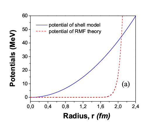
In Fig. 1 we present the potentials vshell​(r)v_{\rm shell}(r) and V1​(r)V_{1}(r) calculated by the approach above.

Refer to caption

Figure 1: (Color online) The potential vshell​(r)v_{\rm shell}(r) of the shell model defined in Eq. (28) (see solid blue line), and the potential of RMF theory V1​(r)V_{1}(r) defined by Eq. (21) and expressed via variable rr (see dashed red line), calculated for the ground state of He4{}^{4}{\rm He}. One can see that both potentials provide only bound states. However, their shapes are essentially different.

From such a picture we see an essential difference between these two potentials. This is the first confirmation of not equivalence in quantum descriptions of nuclear properties and processes provided by the shell model and RMF theory. On such a basis, one can see that difference in quantum description of nuclear processes given by these two potentials given by the shell model and RMF theory should be essential in some cases. Also we obtain:

aξ,0=−2​E1ℏ​wr=−2ℏ​wr​32​ℏ​wr=−3,aξ,1=0,aξ,2=1.\begin{array}[]{lll}a_{\xi,0}=-\displaystyle\frac{2E_{1}}{\hbar w_{r}}=-\displaystyle\frac{2}{\hbar w_{r}}\,\displaystyle\frac{3}{2}\,\hbar w_{r}=-3,&a_{\xi,1}=0,&a_{\xi,2}=1.\end{array} (35)

V Wave functions of nucleons and nucleon densities

V.1 Wave function and density calculations

We shall write a final solution for the wave function of nucleons. Substituting solution (16) for V1​(r)V_{1}(r) to Eqs. (1), (6), we obtain

g⁡(r)=n0​|f0+∑n=1fn​rn|⋅h⁡(r)r,f⁡(r)=−sign⁡[V1​(r)]​n0r​|f0+∑n=1Nfn​rn|​{[f1+∑n=1(n+1)​fn+1​rn2​(f0+∑n=1fn​rn)−1r]​h​(r)+h′​(r)}.\begin{array}[]{lcl}g\,(r)&=&n_{0}\,\sqrt{\Bigl|f_{0}+\displaystyle\sum\limits_{n=1}f_{n}r^{n}\Bigr|}\cdot\displaystyle\frac{h\,(r)}{r},\\ f\,(r)&=&-\,{\rm sign}\,\bigl[V_{1}(r)\bigr]\;\displaystyle\frac{n_{0}}{r\>\sqrt{|f_{0}+\displaystyle\sum\limits_{n=1}^{N}f_{n}r^{n}|}}\;\biggl\{\Bigl[\displaystyle\frac{f_{1}+\displaystyle\sum\limits_{n=1}(n+1)f_{n+1}r^{n}}{2\,(f_{0}+\displaystyle\sum\limits_{n=1}f_{n}r^{n})}-\displaystyle\frac{1}{r}\;\Bigr]\;h\,(r)+h^{\prime}\,(r)\biggr\}.\end{array} (36)

For the ground state of He4{}^{4}{\rm He} we have

g⁡(r)=n0​|V1​(r)|⋅h1​(r)r,f⁡(r)=sign⁡[V1​(r)]​n0|V1​(r)|​{−V1′​(r)2​V1​(r)+rar2}⋅h1​(r)r.\begin{array}[]{lcl}g\,(r)=n_{0}\,\sqrt{\bigl|V_{1}(r)\bigr|}\cdot\displaystyle\frac{h_{1}\,(r)}{r},&f\,(r)={\rm sign}\,\bigl[V_{1}(r)\bigr]\;\displaystyle\frac{n_{0}}{\sqrt{\bigl|V_{1}(r)\bigr|}}\;\biggl\{-\displaystyle\frac{V_{1}^{\prime}(r)}{2\,V_{1}(r)}+\displaystyle\frac{r}{a_{r}^{2}}\biggr\}\cdot\displaystyle\frac{h_{1}\,(r)}{r}.\end{array} (37)

We find the density ρv​(𝐫)\rho_{v}(\mathbf{r}) defined in Eq. (42) in Ref. [2]. For the He4{}^{4}{\rm He} nucleus in the ground state we obtain (n=1n=1, l=0l=0, j=12j=\displaystyle\frac{1}{2}, m=0m=0, M=1/2M=1/2)

ρv​(𝐫)=n02​{|f0+∑n=1fn​rn|+1|f0+∑n=1fn​rn|​|−f1+∑n=1(n+1)​fn+1​rn2​(f0+∑n=1fn​rn)+rar2|2}​h12​(r)r2.\begin{array}[]{lllll}\rho_{v}(\mathbf{r})&=&n_{0}^{2}\,\biggl\{\Bigl|f_{0}+\displaystyle\sum\limits_{n=1}f_{n}r^{n}\Bigr|+\displaystyle\frac{1}{\bigl|f_{0}+\displaystyle\sum\limits_{n=1}f_{n}r^{n}\bigr|}\;\biggl|-\displaystyle\frac{f_{1}+\displaystyle\sum\limits_{n=1}(n+1)f_{n+1}r^{n}}{2\,(f_{0}+\displaystyle\sum\limits_{n=1}f_{n}r^{n})}+\displaystyle\frac{r}{a_{r}^{2}}\biggr|^{2}\biggr\}\,\displaystyle\frac{h_{1}^{2}(r)}{r^{2}}.\end{array} (38)

This solution can be represented in form of series as

ρv​(𝐫)=n02​h2​(r)r2​∑n=0cn​rn.\begin{array}[]{lllll}\rho_{v}(\mathbf{r})&=&n_{0}^{2}\,\displaystyle\frac{h^{2}\,(r)}{r^{2}}\,\displaystyle\sum\limits_{n=0}c_{n}r^{n}.\end{array} (39)

V.2 Calculations of coefficients cnc_{n}

We find the unknown coefficients cnc_{n} in Eq. (39). We combine Eqs. (38) and (39) and obtain the following equation

∑n=0cn​rn=|f0+∑n=1fn​rn|+1|f0+∑n=1fn​rn|​|−f1+∑n=1(n+1)​fn+1​rn2​(f0+∑n=1fn​rn)+rar2|2.\begin{array}[]{lllll}\displaystyle\sum\limits_{n=0}c_{n}r^{n}=\Bigl|f_{0}+\displaystyle\sum\limits_{n=1}f_{n}r^{n}\Bigr|+\displaystyle\frac{1}{\Bigl|f_{0}+\displaystyle\sum\limits_{n=1}f_{n}r^{n}\Bigr|}\;\biggl|-\displaystyle\frac{f_{1}+\displaystyle\sum\limits_{n=1}(n+1)f_{n+1}r^{n}}{2\,(f_{0}+\displaystyle\sum\limits_{n=1}f_{n}r^{n})}+\displaystyle\frac{r}{a_{r}^{2}}\biggr|^{2}.\end{array} (40)

Solving this equation, we obtain the following values for the coefficients (at n≥2n\geq 2, see App. C, for details):

c0=f0+f124​f03,c1=A1​f0−3−3​f0−1​f1​c0,cn=A2​f0−3−f0−3​∑s=1n∑p=0s∑t=0pft​fp−t​fs−p​cn−s,\begin{array}[]{lllll}c_{0}=f_{0}+\displaystyle\frac{f_{1}^{2}}{4f_{0}^{3}},\\ c_{1}=A_{1}f_{0}^{-3}-3f_{0}^{-1}f_{1}\,c_{0},\\ c_{n}=A_{2}f_{0}^{-3}-f_{0}^{-3}\displaystyle\sum\limits_{s=1}^{n}\displaystyle\sum\limits_{p=0}^{s}\displaystyle\sum\limits_{t=0}^{p}f_{t}\,f_{p-t}\,f_{s-p}\,c_{n-s},\end{array} (41)

where

A1=4​f03​f1+f1​f2−1ar2​f0​f1,A2=∑s=0n∑p=0s∑t=0pft​fp−t​fs−p​fn−s+14​∑s=0n(s+1)​(n−s+1)​fs+1​fn−s+1−−1ar2​∑s=0n−1(s+1)​fs+1​fn−s−1+1ar4​∑s=0n−2fs​fn−s−2.\begin{array}[]{lllll}A_{1}&=&4\,f_{0}^{3}f_{1}+f_{1}f_{2}-\displaystyle\frac{1}{a_{r}^{2}}f_{0}f_{1},\\ A_{2}&=&\displaystyle\sum\limits_{s=0}^{n}\displaystyle\sum\limits_{p=0}^{s}\displaystyle\sum\limits_{t=0}^{p}f_{t}\,f_{p-t}\,f_{s-p}\,f_{n-s}+\displaystyle\frac{1}{4}\,\displaystyle\sum\limits_{s=0}^{n}(s+1)(n-s+1)\,f_{s+1}f_{n-s+1}-\\ &-&\displaystyle\frac{1}{a_{r}^{2}}\displaystyle\sum\limits_{s=0}^{n-1}(s+1)\,f_{s+1}f_{n-s-1}+\displaystyle\frac{1}{a_{r}^{4}}\,\displaystyle\sum\limits_{s=0}^{n-2}f_{s}f_{n-s-2}.\end{array} (42)

From the obtained solutions we see, that these coefficients do not depend explicitly on factor n0n_{0}. However, such a dependence is included in calculations of coefficients fnf_{n} in Eqs. (18).

In Fig. 2 we present our calculations of the wave functions and densities provided by the shell model and RMF theory for the ground state of He4{}^{4}{\rm He}.

Refer to caption Refer to caption

Figure 2: (Color online) The nucleon radial wave functions and the densities of the shell model and RMF theory for the He4{}^{4}{\rm He} nucleus in the ground state. Panel a: The wave function h1​(r)h_{1}(r) of the shell model defined in Eq. (32) at n=1n=1 for the ground state (see solid blue line), the wave function r​g​(r)r\,g(r) of the RMF theory defined in Eq. (36) and re-scaled on maximum of the function h1​(r)h_{1}(r) (see dashed red line), and the wave function r​f​(r)r\,f(r) of the RMF theory defined in Eq. (36) and re-scaled on maximum of the function h1​(r)h_{1}(r) (see dash-dotted green line). One case see difference in the shapes of theses wave functions: we observe a clear radial distance between maximums of the function of the shell model [h1​(rmax)=8.31769​MeV1/2h_{1}(r_{\rm max})=8.31769\,{\rm MeV}^{1/2} at rmax=1.2024r_{\rm max}=1.2024 fm] and functions of RMF theory [rmax​g​(rmax)=162.29505​MeV1/2r_{\rm max}\,g(r_{\rm max})=162.29505\,{\rm MeV}^{1/2} at rmax=4.64930r_{\rm max}=4.64930 fm, and rmax​f​(rmax)=8.73757⋅108​MeV1/2r_{\rm max}\,f(r_{\rm max})=8.73757\cdot 10^{8}\,{\rm MeV}^{1/2} at rmax=4.32866r_{\rm max}=4.32866 fm]. From here we conclude that a probability of nucleons described by the wave function f⁡(r)f(r) is essentially larger than the probability given by the function g⁡(r)g(r). So, for more quick calculations we can recommend to use only the function f⁡(r)f(r) in analysis of quantum properties of this nucleus. Panel b: The nucleon density of the shell model defined as ρv​(r)=h12​(r)/r2\rho_{v}(r)=h_{1}^{2}\,(r)/r^{2} (see solid blue line), the nucleon density ρv​(r)\rho_{v}(r) of the RMF theory defined in Eq. (38) (see dashed red line, its maximum is at 3.967943.96794 fm) (the densities are re-scaled on unite at maximums). One can see clear difference between maximums of both lines which describes different nucleon distributions inside the nucleus given by the shell model and RMF theory. Such a difference is explained by appearance of the additional factor |V1​(r)|1/2|V_{1}(r)|^{1/2} in the radial wave function g⁡(r)g(r) and the corresponding factor |V1|−1/2(−V1′/(2V1)+rar−2)|V_{1}|^{-1/2}\,(-V_{1}^{\prime}/(2V_{1})+ra_{r}^{-2}) in the radial wave function f⁡(r)f(r) [see Eqs. (37)].

One can see that these two approaches give essentially different probabilities of nucleons in dependence on the radial distance, which provide principally different physical description of quantum picture of nucleon distribution inside this nucleus. From such a picture, the nucleon densities given by RMF theory contradict to knowledge about distribution of the proton and neutron densities inside the nuclei obtained from experimental study of scattering of high energetic electrons off nuclei, spectroscopic information about transitions in muon atoms, isotopic and isomer shifts in the optical spectra (see Refs. [61, 62, 63]). This strongly indicate that the functions gg and ff have no sense as the wave functions provided by quantum physics. At the same time, the function hh which is connected with these two functions above, provides us a proper description of quantum properties of nucleons inside the He4{}^{4}{\rm He} nucleus.

Refer to caption

Figure 3: (Color online) The nucleon densities of the RMF theory. The density ρv​(r)\rho_{v}(r) is defined in Eq. (38) (see dashed red line), the density ρv​(r)\rho_{v}(r) is defined in series expansion approach (39) with coefficients determined by Eqs. (41) and  (42) (see solid dark cyan line) (the densities are re-normalized on unite at maximums). A difference between shapes is explained by the accuracy of the series expansion approach (that characterizes accuracy of determination of coefficients in Eqs. (41) and  (42)).

VI Solution of equations for mesons

In this section we shall find solution of the system of equations for mesons ww defined in Eq. (38) in Ref. [2].

(−△+mw)​w0​(𝐫)=gw​ρv​(𝐫).(-\triangle+m_{w})\,w^{0}(\mathbf{r})=g_{w}\,\rho_{v}(\mathbf{r}). (43)

We shall rewrite the nucleon density in the right part of this equation in form of series expansion as (39) and we use the following form for the unknown function

w0​(r,θ,ϕ)=Rw​(r)​Yl​m​(θ,ϕ),Rw​(r)=χw​(r)r.\begin{array}[]{lcl}w^{0}(r,\theta,\phi)=R_{w}(r)\,Y_{lm}(\theta,\phi),&R_{w}(r)=\displaystyle\frac{\chi_{w}(r)}{r}.\end{array} (44)

Then the left part of Eq. (43) is transformed into

{−d2d​r2+l⁡(l+1)r2+mw2}​χw​(r)​Yl​m​(θ,ϕ)=gw​ρv​(𝐫)​r.\begin{array}[]{lcl}\Bigl\{-\displaystyle\frac{d^{2}}{dr^{2}}+\displaystyle\frac{l(l+1)}{r^{2}}+m_{w}^{2}\Bigr\}\,\chi_{w}(r)\,Y_{lm}(\theta,\phi)=g_{w}\,\rho_{v}(\mathbf{r})\;r.\end{array} (45)

As the density function ρv​(𝐫)\rho_{v}(\mathbf{r}) has no angular part, this equation has solution only in case of l=0l=0 (we are interesting in such a case). So, Eq. (45) is transformed to one-dimensional

{−d2d​r2+mw2}​χw​(r)=gw​ρv​(𝐫)​r.\begin{array}[]{lcl}\Bigl\{-\displaystyle\frac{d^{2}}{dr^{2}}+m_{w}^{2}\Bigr\}\,\chi_{w}(r)=g_{w}\,\rho_{v}(\mathbf{r})\;r.\end{array} (46)

We look for the unknown function χw​(r)\chi_{w}(r) in form of the series expansion as

χw​(r)=n02​h2​(r)r​∑n=0cw,n​rn,\begin{array}[]{lllll}\chi_{w}(r)&=&n_{0}^{2}\,\displaystyle\frac{h^{2}(r)}{r}\,\displaystyle\sum\limits_{n=0}c_{w,n}r^{n},\end{array} (47)

where cw,nc_{w,n} are new unknown coefficients. We calculate derivatives, rewrite Eq. (46) as

−χw′′​(r)+mw2​χw=−n02h2​(r)r{2​cw,1r+6[cw,2−ar−2cw,0]+[12cw,3−10ar−2cw,1]r−+∑n=2[4ar−4cw,n−2−2ar−2(2n+3)cw,n+(n+2)(n+3)cw,n+2]rn}+mw2n02h2​(r)r∑n=0cw,nrn==gw​ρv​(𝐫)​r=gw​n02​h2​(r)r​∑n=0cn​rn.\begin{array}[]{lllll}\vskip 1.42262pt-\chi_{w}^{\prime\prime}(r)+m_{w}^{2}\chi_{w}&=&-n_{0}^{2}\,\displaystyle\frac{h^{2}(r)}{r}\;\biggl\{\displaystyle\frac{2\,c_{w,1}}{r}+6\,\bigl[c_{w,2}-a_{r}^{-2}c_{w,0}\bigr]+\bigl[12\,c_{w,3}-10a_{r}^{-2}c_{w,1}\bigr]\,r\;-\\ &+&\displaystyle\sum\limits_{n=2}\Bigl[4a_{r}^{-4}c_{w,n-2}-2a_{r}^{-2}(2n+3)\,c_{w,n}+(n+2)\,(n+3)\,c_{w,n+2}\Bigr]\,r^{n}\biggr\}\;+\;\par m_{w}^{2}\,n_{0}^{2}\displaystyle\frac{h^{2}(r)}{r}\displaystyle\sum\limits_{n=0}c_{w,n}r^{n}\;=\\ &=&g_{w}\,\rho_{v}(\mathbf{r})\;r=g_{w}\;n_{0}^{2}\,\displaystyle\frac{h^{2}\,(r)}{r}\,\displaystyle\sum\limits_{n=0}c_{n}r^{n}.\end{array} (48)

and find the unknown coefficients (see App. D, for details)

cw,1=0,cw,2=(ar−2+mw26)​cw,0−gw6​c0,cw,3=−gw12​c1,cw,n+2=−4​ar−4(n+2)​(n+3)​cw,n−2+2​ar−2​(2​n+3)+mw2(n+2)​(n+3)​cw,n−gw(n+2)​(n+3)​cn.\begin{array}[]{lllll}\vskip 5.69054ptc_{w,1}=0,\\ \vskip 5.69054ptc_{w,2}=\Bigl(a_{r}^{-2}+\displaystyle\frac{m_{w}^{2}}{6}\Bigr)\,c_{w,0}-\displaystyle\frac{g_{w}}{6}\,c_{0},\\ \vskip 5.69054ptc_{w,3}=-\displaystyle\frac{g_{w}}{12}\,c_{1},\\ c_{w,n+2}=-\displaystyle\frac{4a_{r}^{-4}}{(n+2)\,(n+3)}\,c_{w,n-2}+\displaystyle\frac{2a_{r}^{-2}(2n+3)+m_{w}^{2}}{(n+2)\,(n+3)}\,c_{w,n}-\displaystyle\frac{g_{w}}{(n+2)\,(n+3)}\,c_{n}.\end{array} (49)

From such solutions we see that there is arbitrary choice in determination of cw,0c_{w,0}. In Fig. 4 we present our calculation of the radial component of the meson wave function, Rw​(r)R_{w}(r), given by Eqs. (44) and (47).

Refer to caption

Figure 4: (Color online) The meson radial wave function Rw​(r)R_{w}(r) defined by Eqs. (44) and (47) where the coefficients cw,nc_{w,n} are determined by Eqs. (49) [maximum of this function is Rw​(rmax)=0.17198​MeV3R_{w}(r_{\rm max})=0.17198\,{\rm MeV}^{3} at rmax=4.32866r_{\rm max}=4.32866 fm, we use cw,0=1c_{w,0}=1 in calculations]. One can observe similarity (after re-scaling) of its shape with the shape of the nucleon density given in Figs. 2(b) and 3.

But in practical calculations, varying cw,0c_{w,0} the shape of the meson wave function Rw​(r)R_{w}(r) keeps to be stable (after re-scaling). At r→0r\to 0, the function χw​(r)→0\chi_{w}(r)\to 0 independently on choice of cw,0c_{w,0}.

VII Quantum correction to the potential

The meson function w0w_{0} was defined in Eqs. (44), (47) and (49) on the basis of solution (41) for the wave function ψε​j​l​M​(𝐫)\psi_{\varepsilon jlM}(\mathbf{r}) in Eqs. (2) and (3) and the potential V1V_{1} in Eqs. (21), (22) which are in direct correspondence with the wave function and potential (30) and (31) of the shell model. So, the potential V⁡(r)V(r) defined in Eq. (45) in Ref. [2] on the basis of the found meson wave function w0w_{0}, is connected with wave function ψε​j​l​M​(𝐫)\psi_{\varepsilon jlM}(\mathbf{r}) but this wave functions is not exact solution for this potential in Dirac Eq. (1). On the other side, we found the potential V1V_{1} which is directly connected with the potential of the shell model. If the meson theory describes quantum properties of nucleus well (like the shell model), then a difference between these two potentials should be as small as possible (tend to zero). In order to analyze this, we introduce new quantum corrections characterizing difference between these two potentials. In order to provide the first estimations and realize this idea as clear as possible, we restrict ourselves by the potential V⁡(r)V(r) without terms gρ​τ3​ρ30​(𝐫)g_{\rho}\tau_{3}\rho_{3}^{0}(\mathbf{r}) and ε​A0​(𝐫)\varepsilon\,A^{0}(\mathbf{r}) (electromagnetic interactions). We formulate the corrections, generalizing the potential V⁡(r)V(r) defined in Eq. (45) in Ref. [2] as

Vgen​(r)=gquant,w​gw​w0​(r)+Δ​V​(r)+V0,V_{\rm gen}(r)=g_{\rm quant,w}\,g_{w}\,w^{0}(r)+\Delta V(r)+V_{0}, (50)

where we introduced a new factor gquant,wg_{\rm quant,w}, a new function Δ​V​(r)\Delta V(r), and a new constant V0V_{0}. In order to find these new corrections, we introduce the following requirement: Correction Δ​V​(r)\Delta V(r) should be minimal. In result, we obtain:

Δ​V​(r)=V1​(r)−vw​(r),vw​(r)=gquant,w​gw​w0​(r),V0=ε1+m,\begin{array}[]{lllll}\vskip 5.69054pt\Delta V(r)=V_{1}(r)-v_{w}(r),&v_{w}(r)=g_{\rm quant,w}\,g_{w}\,w^{0}(r),&V_{0}=\varepsilon_{1}+m,\end{array} (51)

where ε1\varepsilon_{1} is energy of nucleon in the the ground state, and we introduce a new function vw​(r)v_{w}(r) for more easy demonstration of the meson potential.

Before the calculations of the quantum corrections, at first we analyze how much closely these two potentials V1​(r)V_{1}(r) and vw​(r)v_{w}(r) can be located, if to vary the factor gquant,wg_{\rm quant,w}. Results of such calculations are presented in Fig. 5.

Refer to caption Refer to caption

Figure 5: (Color online) The nucleon potential V1​(r)V_{1}(r) defined in Eqs. (21), (22) and the re-normalized meson potential vw​(r)v_{w}(r) defined in Eq. (51). We find an unknown new factor gquant,wg_{\rm quant,w} from condition of coincidence V1​(r0)=vw​(r0)V_{1}(r_{0})=v_{w}(r_{0}) at the radial point of intersection r0r_{0} for the ground state (here, r0=3​arr_{0}=\sqrt{3}\,a_{r}, see Fig. 1). We obtain gquant,w=2.3864127⋅106g_{\rm quant,w}=2.3864127\cdot 10^{6}. This indicates that the initial potential V1V_{1} should be strongly reinforced in order to minimize maximally the additional quantum correction Δ​V\Delta V. Another conclusion is that without inclusion of this quantum correction, the potential of the RMF theory defined in Eq. (45) in Ref. [2] is far from quantum description of properties of the nucleus He4{}^{4}{\rm He} given by the shell model. Panel a: One can see that difference between these two potentials is very small inside a small radial region at r≤r0r\leq r_{0}. Panel b: For large radial distance, at r≥r0r\geq r_{0}, difference between these two functions is highly increased with increasing of radius rr. One can see that the quantum correction Δ​V​(r)\Delta V(r) is practically determined only by the potential V1​(r)V_{1}(r) in this region. A next conclusion is that after inclusion of the new factor qquantum,wq_{\rm quantum,w} (and without adding Δ​V​(r)\Delta V(r)), the modified meson potential vw​(r)v_{w}(r) can be successful in description of the quantum properties (on the level of the shell model) for analyzing nucleus He4{}^{4}{\rm He} for energies below the ground state or a little above. It is impossible to describe the quantum properties properly for the energies higher than the ground state energy level without inclusion of the quantum corrections Δ​V​(r)\Delta V(r). This demonstrates clearly an importance of introduction of the quantum corrections in this paper to the existed RMF theory.

We find that these two functions can be intersected at point r0=3​arr_{0}=\sqrt{3}\,a_{r} (and, so, we use this condition for determination of gquant,wg_{\rm quant,w}). The final calculated quantum correction Δ​V​(r)\Delta V(r) is presented in Fig. 6 in comparison on the potential V1V_{1}.

Refer to caption Refer to caption

Figure 6: (Color online) The quantum correction Δ​V​(r)\Delta V(r) defined in Eq. (51) and the potential V1V_{1}. Panel a: Blue solid line is for the correction Δ​V\Delta V, red dashed line is for the potential V1V_{1}. One can see that the quantum correction is very small at r≤r0r\leq r_{0} (this function is negative in this region), but it is increased highly at r≥r0r\geq r_{0}. Panel b: Ratio |V1​(r)−Δ​V​(r)|/V1​(r)|V_{1}(r)-\Delta V(r)|/V_{1}(r).

One can see that at r≤r0r\leq r_{0} the quantum correction Δ​V\Delta V is very small, but it is increased highly at increasing rr at r>r0r>r_{0}.

VIII Conclusions

In this paper, we have compared the RMF theory [2, 3, 4, 5, 6, 7, 8] and the microscopic model [38, 39, 40, 41] in description of the quantum properties of the light nuclei in the bound states in the spherically symmetric approximation. We have obtained an explicit analytical relation between differential equations for the RMF theory and the model of deformed shells, which determine wave functions for nucleons. On such a basis we perform analysis of correspondence of quantum properties of nuclei described by these wave functions. Conclusions from analysis on the basis of this approach are the following.

  1. 1.

    On the basis of the found relations above, we found the potential VR​M​FV_{RMF} of the RMF theory for nucleons [see Eqs. (19), (21) and (22)] which provides solutions of the wave functions for nucleons, coincident exactly analytically with solutions for the nucleon wave function given by the DOS model. This fact confirms that it is possible to describe quantum properties of nucleus in framework of the RMF theory exactly the same as in the DOS model. Note the following.

    1. (a)

      However, we find that a difference between the potential VR​M​FV_{RMF} of the RMF theory and the corresponding potential Vs​h​e​l​lV_{shell} of the DOS model is essential for any nucleus. On example of the He4{}^{4}{\rm He} nucleus in the ground state, we find that a maximal relative difference between the potentials is for the radius values near zero, 1.6 fm and for region larger 2 fm (see Fig. 1).

    2. (b)

      For determination of the unknown potential VR​M​FV_{RMF} we introduce a series expansion approach [see Eqs. (21) and (22)] which is effective in next calculations of the unknown wave functions for nucleons and densities, solution of equations for mesons. However, this approach provides arbitrary choice of the first unknown coefficient f0f_{0} (which changes the potential VR​M​FV_{RMF}). To resolve this problem, we formulate a new condition: The ground states should be equivalent in frameworks of the DOS model and RMF theory (see Eq. (34) for the found coefficient f0f_{0} for He4{}^{4}{\rm He} on this basis).

  2. 2.

    The wave functions for the nucleons and the nucleon densities obtained by the DOS model and RMF theory are essentially different. On example of the He4{}^{4}{\rm He} nucleus in the ground state we observe a clear radial distance between maximums of the function of the DOS model [h1​(rmax)=8.31769​MeV1/2h_{1}(r_{\rm max})=8.31769\,{\rm MeV}^{1/2} at rmax=1.2024r_{\rm max}=1.2024 fm] and functions of RMF theory [rmax​g​(rmax)=162.29505​MeV1/2r_{\rm max}\,g(r_{\rm max})=162.29505\,{\rm MeV}^{1/2} at rmax=4.64930r_{\rm max}=4.64930 fm, and rmax​f​(rmax)=8.73757⋅108​MeV1/2r_{\rm max}\,f(r_{\rm max})=8.73757\cdot 10^{8}\,{\rm MeV}^{1/2} at rmax=4.32866r_{\rm max}=4.32866 fm] (see Fig. 2). We conclude the following.

    • •

      Such a difference is explained by appearance of the additional factor |V1​(r)|1/2|V_{1}(r)|^{1/2} in the radial wave function g⁡(r)g(r) and the corresponding factor |V1|−1/2(−V1′/(2V1)+rar−2)|V_{1}|^{-1/2}\,(-V_{1}^{\prime}/(2V_{1})+ra_{r}^{-2}) in the radial wave function f⁡(r)f(r) [see Eqs. (37)].

    • •

      A probability of nucleons described by the wave function f⁡(r)f(r) is essentially larger than the probability given by the function g⁡(r)g(r). So, for more quick (simple) calculations we can recommend to use only the function f⁡(r)f(r) in analysis of quantum properties of this nucleus.

    • •

      The nucleon densities given by RMF theory contradict to knowledge about distribution of the proton and neutron densities inside the nuclei obtained from experimental study of scattering of high energetic electrons off nuclei, spectroscopic information about transitions in muon atoms, isotopic and isomer shifts in the optical spectra (see Refs. [61, 62, 63]). This indicates that the functions gg and ff have no sense as the wave functions of quantum physics. At the same time, the function hh which is part of these two functions above, provides us a proper description of quantum properties of nucleons inside the nucleus.

  3. 3.

    We calculate meson function w0​(𝐫)w^{0}(\mathbf{r}) (see Eqs. (44), (47) and (49)) which corresponds to the found nucleon density above (see Fig. 4). We observe similarity of its radial shape (after re-scaling) with the shape of the nucleon radial density given in Figs. 2(b) and 3.

  4. 4.

    The potential V⁡(r)V(r) defined in Eq. (45) in Ref. [2] on the basis of the found meson wave function w0w_{0} above, is connected with the wave function ψε​j​l​M​(𝐫)\psi_{\varepsilon jlM}(\mathbf{r}) in Eqs. (2) and (3) but this wave functions is not exact solution of Dirac Eqs. (1) with this potential. On the other side, we found the potential V1V_{1} which is directly connected with the potential of the DOS model. If the meson theory describes quantum properties of nucleus well, then a difference between these two potentials should be as small as possible (tend to zero). In order to analyze this, we introduce new quantum corrections gquant,wg_{\rm quant,w}, Δ​V​(r)\Delta V(r), and V0V_{0} in Eq. (50) characterizing difference between these two potentials [we restrict ourselves by the potential V⁡(r)V(r) without terms gρ​τ3​ρ30​(𝐫)g_{\rho}\tau_{3}\rho_{3}^{0}(\mathbf{r}) and ε​A0​(𝐫)\varepsilon\,A^{0}(\mathbf{r}) (electromagnetic interactions)]. In order to find these new corrections, we introduce the following requirement: Correction Δ​V​(r)\Delta V(r) should be minimal. Using this condition, we find the following.

    1. (a)

      The potentials V1​(r)V_{1}(r) and vw​(r)v_{w}(r) are very close and are intersected at point r0=3​arr_{0}=\sqrt{3}\,a_{r} (see Fig. 5). The difference between these two potentials is very small inside a small radial region at r≤r0r\leq r_{0}, but at r≥r0r\geq r_{0} it is highly increased at increasing radius rr. The quantum correction Δ​V​(r)\Delta V(r) is practically determined only by the potential V1​(r)V_{1}(r) in this region.

    2. (b)

      We find an unknown new factor gquant,wg_{\rm quant,w} from condition of coincidence V1​(r0)=vw​(r0)V_{1}(r_{0})=v_{w}(r_{0}) at the radial point of intersection r0r_{0} for the ground state (here, r0=3​arr_{0}=\sqrt{3}\,a_{r}, see Fig. 1). We obtain gquant,w=2.3864127⋅106g_{\rm quant,w}=2.3864127\cdot 10^{6}. This indicates that the initial potential V1V_{1} (and meson function w0w^{0}) should be strongly reinforced in order to minimize maximally the additional correction Δ​V\Delta V.

    3. (c)

      After inclusion of the factor qquantum,wq_{\rm quantum,w} (and without adding Δ​V​(r)\Delta V(r)), the modified meson potential vw​(r)v_{w}(r) can be successful in description of the quantum properties (on the level of the shell model) for analyzing nucleus He4{}^{4}{\rm He} for energies below the ground state or a little above (for scattering processes). It is impossible to describe the quantum properties properly for the energies higher than the ground state energy level without inclusion of the quantum corrections Δ​V​(r)\Delta V(r). This demonstrates an importance of introduction of the quantum corrections to the RMF theory.

    4. (d)

      Introduction of the correction Δ​V​(r)\Delta V(r) allows to describe completely the quantum properties of the nucleus He4{}^{4}{\rm He}, as in the DOS model. The shape of the correction Δ​V​(r)\Delta V(r) is presented in Fig. 6. One can see that at r≤r0r\leq r_{0} the correction Δ​V\Delta V is very small, but it is increased highly at increasing rr at r>r0r>r_{0}.

At finishing, we should like to note that the approach proposed in this paper opens a new perspective of next application of methods of quantum mechanics (oriented on high accuracy in detailed description and study of quantum properties in nuclear physic) to the tasks of the RMF theory (for example, see Ref. [64] for details).

Acknowledgements

S. P. M. thanks the Institute of Modern Physics of Chinese Academy of Sciences for its warm hospitality and support. This work has been supported by the Major State Basic Research Development Program in China (No. 2015CB856903), the National Natural Science Foundation of China (Grant Nos. 11575254, 11447105 and 11175215), the Chinese Academy of Sciences fellowships for researchers from developing countries (No. 2014FFJA0003), and the Chinese Academy of Sciences President’s International Fellowship Initiative (No. 2015PM062).

Appendix A Transition from the radial Dirac equation to one-dimensional differential equation of the second order (type of equation of Schrödinger-like form)

Let us consider equation of Dirac

i​ℏ​∂Ψ∂t=H^​Ψi\,\hbar\displaystyle\frac{\partial\Psi}{\partial t}=\hat{H}\Psi (52)

with Hamiltonian of form:

H^=α​𝐩+β​m+V⁡(r),\hat{H}=\alpha\mathbf{p}+\beta m+V(r), (53)

where V⁡(r)V(r) is potential energy, dependent on the radial variable rr, α\alpha and β\beta are ÷åòûðåõðÿäíûå matrixes of Dirac, 𝐩=−i∂/∂𝐫\mathbf{p}=-i\,\partial/\partial\mathbf{r} is operator of momentum of the particle, mm is mass of the particle. We choose a system of units where c=ℏ=1c=\hbar=1 (i. e. we shall omit these constants sometimes).

We shall find a solution for the wave function in form (see Sect. 1.5.1, page 48 in [60]):

Ψ(𝐫,t)=ψε​j​l​M(𝐫)⋅e−iεt/ℏ,ψε​j​l​M​(𝐫)=(φε​j​l​M​(𝐫)χε​j​l​M​(𝐫)),\begin{array}[]{lcl}\Psi(\mathbf{r},t)=\psi_{\varepsilon jlM}(\mathbf{r})\cdot e^{-i\varepsilon t/\hbar},&\psi_{\varepsilon jlM}(\mathbf{r})=\left(\begin{array}[]{lcl}\varphi_{\varepsilon jlM}(\mathbf{r})\\ \chi_{\varepsilon jlM}(\mathbf{r})\end{array}\right),\end{array} (54)

where

φε​j​l​M​(𝐫)=g⁡(r)​Ωj​l​M​(𝐧),χε​j​l​M​(𝐫)=i​f​(r)​Ωj​l′​M​(𝐧)\begin{array}[]{lcl}\varphi_{\varepsilon jlM}(\mathbf{r})=g\,(r)\;\Omega_{jlM}(\mathbf{n}),&\chi_{\varepsilon jlM}(\mathbf{r})=i\,f\,(r)\;\Omega_{jl^{\prime}M}(\mathbf{n})\end{array} (55)

and Ωj​l​M​(𝐧)\Omega_{jlM}(\mathbf{n}) is spherical harmonic spinor (called also as spherical harmonic spinor function), l′=2​j−ll^{\prime}=2j-l, 𝐧=𝐫/r\mathbf{n}=\mathbf{r}/r, r=|𝐫|r=|\mathbf{r}|, g⁡(r)g\,(r) and f⁡(r)f\,(r) are radial functions. According to [60], ε\varepsilon is eigenvalue of Hamiltonian (but not energy of the particle), which can be positive and negative. At ε>0\varepsilon>0, the equation describes particle, at ε<0\varepsilon<0 — antiparticle. The energy is defined as E=|ε|E=|\varepsilon|, i. e. it is positive for the particles, and for the antiparticles. Substituting formulas (54) and (55) for the wave function into equation (52), we obtain system of two equations for the radial functions (see (1.5.4), page 49 in [60]):

d⁡(r​g​(r))d​r+χr​(r​g​(r))−[ε+m−V⁡(r)]​(r​f​(r))=0,d⁡(r​f​(r))d​r−χr​(r​f​(r))+[ε−m−V⁡(r)]​(r​g​(r))=0,\begin{array}[]{lcl}\vskip 5.69054pt\displaystyle\frac{d\,(rg(r))}{dr}+\displaystyle\frac{\chi}{r}\,(rg(r))-\bigl[\varepsilon+m-V(r)\bigr]\,(rf(r))=0,\\ \displaystyle\frac{d\,(rf(r))}{dr}-\displaystyle\frac{\chi}{r}\,(rf(r))+\bigl[\varepsilon-m-V(r)\bigr]\,(rg(r))=0,\end{array} (56)

where χ=l⁡(l+1)−j⁡(j+1)−1/4\chi=l(l+1)-j(j+1)-1/4 (see (1.4.6), page 44 in [60]). From this system we remove ff, in order to obtain equation for determination of gg. From the first equation we find:

r​f​(r)=1ε+m−V⁡(r)​{d⁡(r​g​(r))d​r+χr​(r​g​(r))}\begin{array}[]{lcl}rf(r)&=&\displaystyle\frac{1}{\varepsilon+m-V(r)}\,\Bigl\{\displaystyle\frac{d\,(rg(r))}{dr}+\displaystyle\frac{\chi}{r}\,(rg(r))\Bigr\}\end{array} (57)

and derivative from this function:

d⁡(r​f​(r))d​r=dd​r​[1ε+m−V⁡(r)​{d⁡(r​g​(r))d​r+χr​(r​g​(r))}]==1ε+m−V⁡(r)​d2​(r​g​(r))d​r2+[1(ε+m−V⁡(r))2​d​V​(r)d​r+1ε+m−V⁡(r)​χr]​d⁡(r​g​(r))d​r++[1(ε+m−V⁡(r))2​χr​d​V​(r)d​r−1ε+m−V⁡(r)​χr2]​(r​g​(r)).\begin{array}[]{lcl}\vskip 5.69054pt\displaystyle\frac{d\,(rf(r))}{dr}&=&\displaystyle\frac{d}{dr}\,\biggl[\displaystyle\frac{1}{\varepsilon+m-V(r)}\,\Bigl\{\displaystyle\frac{d\,(rg(r))}{dr}+\displaystyle\frac{\chi}{r}\,(rg(r))\Bigr\}\biggr]=\\ &=&\displaystyle\frac{1}{\varepsilon+m-V(r)}\,\displaystyle\frac{d^{2}\,(rg(r))}{dr^{2}}+\biggl[\displaystyle\frac{1}{(\varepsilon+m-V(r))^{2}}\,\displaystyle\frac{dV(r)}{dr}+\displaystyle\frac{1}{\varepsilon+m-V(r)}\,\displaystyle\frac{\chi}{r}\biggr]\,\displaystyle\frac{d\,(rg(r))}{dr}+\\ &+&\biggl[\displaystyle\frac{1}{(\varepsilon+m-V(r))^{2}}\,\displaystyle\frac{\chi}{r}\,\displaystyle\frac{dV(r)}{dr}-\displaystyle\frac{1}{\varepsilon+m-V(r)}\,\displaystyle\frac{\chi}{r^{2}}\biggr](rg(r)).\end{array} (58)

We substitute these formulas into the second equation of the system (56), and obtain:

d2​(r​g​(r))d​r2+1ε+m−V⁡(r)​d​V​(r)d​r​d⁡(r​g​(r))d​r+F⁡(r)​(r​g​(r))=0,\begin{array}[]{cl}&\displaystyle\frac{d^{2}\,(rg(r))}{dr^{2}}+\displaystyle\frac{1}{\varepsilon+m-V(r)}\,\displaystyle\frac{dV(r)}{dr}\,\displaystyle\frac{d\,(rg(r))}{dr}\;+\;F(r)\,(rg(r))=0,\end{array} (59)

where a new function was introduced:

F⁡(r)=1ε+m−V⁡(r)​χr​d​V​(r)d​r−χ⁡(1+χ)r2+[ε−V⁡(r)]2−m2.F(r)=\displaystyle\frac{1}{\varepsilon+m-V(r)}\,\displaystyle\frac{\chi}{r}\,\displaystyle\frac{dV(r)}{dr}-\displaystyle\frac{\chi(1+\chi)}{r^{2}}+\bigl[\varepsilon-V(r)\bigr]^{2}-m^{2}. (60)

Now we use change:

r​g​(r)=a⁡(r)​h​(r),r\,g(r)=a(r)\,h(r), (61)

from where we find:

(r​g​(r))′=a′​(r)​h​(r)+a⁡(r)​h​(r)′,(r​g​(r))′′=a′′​(r)​h​(r)+2​a′​(r)​h′​(r)+a⁡(r)​h​(r)′′.\begin{array}[]{cc}(r\,g(r))^{\prime}=a^{\prime}(r)\,h(r)+a(r)\,h(r)^{\prime},&(r\,g(r))^{\prime\prime}=a^{\prime\prime}(r)\,h(r)+2a^{\prime}(r)\,h^{\prime}(r)+a(r)\,h(r)^{\prime\prime}.\end{array} (62)

Then, we shall rewrite equation (59) in form:

a′′​h+ 2​a′​h′+a​h′′+1ε+m−V​d​Vd​r​{a′​h+a​h′}+F​a​h=0.a^{\prime\prime}\,h\;+\;2a^{\prime}\,h^{\prime}\;+\;a\,h^{\prime\prime}\;+\;\displaystyle\frac{1}{\varepsilon+m-V}\,\displaystyle\frac{dV}{dr}\Bigl\{a^{\prime}\,h+a\,h^{\prime}\Bigr\}\;+\;F\,a\,h=0. (63)

Let us transform further as

h′′+{ 2​a′a+V′ε+m−V}​h′+{a′′a+V′ε+m−V​a′a+F}​h=0.h^{\prime\prime}+\Bigl\{\ 2\,\displaystyle\frac{a^{\prime}}{a}+\displaystyle\frac{V^{\prime}}{\varepsilon+m-V}\,\Bigr\}\,h^{\prime}+\Bigl\{\ \displaystyle\frac{a^{\prime\prime}}{a}+\displaystyle\frac{V^{\prime}}{\varepsilon+m-V}\,\displaystyle\frac{a^{\prime}}{a}+F\Bigr\}\,h=0. (64)

From this equation we formulate a new condition for determination of the unknown function a⁡(r)a(r):

2​a′a+V′ε+m−V=0.2\,\displaystyle\frac{a^{\prime}}{a}+\displaystyle\frac{V^{\prime}}{\varepsilon+m-V}=0. (65)

Then, equation (64) is transformed to

h′′+{a′′a+V′ε+m−V​a′a+F}​h=0.\begin{array}[]{cc}h^{\prime\prime}+\Bigl\{\ \displaystyle\frac{a^{\prime\prime}}{a}+\displaystyle\frac{V^{\prime}}{\varepsilon+m-V}\,\displaystyle\frac{a^{\prime}}{a}+F\Bigr\}\,h=0.\end{array} (66)

We rewrite it in the final form, introducing a new potential function (and taking eq. (65) into account):

−h′′+V¯​(r)​h=0,-\,h^{\prime\prime}+\bar{V}(r)\,h=0, (67)

where

V¯​(r)=−a′′a+12​{V′ε+m−V}2−V′ε+m−V⁡(r)​χr−[ε−V⁡(r)]2+m2+χ⁡(1+χ)r2.\begin{array}[]{cc}\bar{V}(r)=-\,\displaystyle\frac{a^{\prime\prime}}{a}+\displaystyle\frac{1}{2}\,\Bigl\{\displaystyle\frac{V^{\prime}}{\varepsilon+m-V}\,\Bigr\}^{2}-\displaystyle\frac{V^{\prime}}{\varepsilon+m-V(r)}\,\displaystyle\frac{\chi}{r}\,-\bigl[\varepsilon-V(r)\bigr]^{2}+m^{2}+\displaystyle\frac{\chi(1+\chi)}{r^{2}}.\end{array} (68)

From Eq. (65) we find:

a′′a=−V′′2​(ε+m−V)−(V′)24​(ε+m−V)2.\begin{array}[]{l}\displaystyle\frac{a^{\prime\prime}}{a}=-\displaystyle\frac{V^{\prime\prime}}{2\,(\varepsilon+m-V)}-\displaystyle\frac{(V^{\prime})^{2}}{4\,(\varepsilon+m-V)^{2}}.\end{array} (69)

Substituting this formula to eq. (68), we find:

V¯​(r)=V′′2​(ε+m−V)+3​(V′)24​(ε+m−V)2−V′ε+m−V⁡(r)​χr−[ε−V⁡(r)]2+m2+χ⁡(1+χ)r2.\begin{array}[]{cc}\bar{V}(r)=\displaystyle\frac{V^{\prime\prime}}{2\,(\varepsilon+m-V)}+\displaystyle\frac{3\,(V^{\prime})^{2}}{4\,(\varepsilon+m-V)^{2}}-\displaystyle\frac{V^{\prime}}{\varepsilon+m-V(r)}\,\displaystyle\frac{\chi}{r}\,-\bigl[\varepsilon-V(r)\bigr]^{2}+m^{2}+\displaystyle\frac{\chi(1+\chi)}{r^{2}}.\end{array} (70)

Now we shall obtain the wave function. From eq. (65) we find a solution for aa (we shall consider case of a>0a>0)55 5 at ε+m−V<0\varepsilon+m-V<0 we have the same formula: 2​a′a=(ln⁡a2)′=−V′ε+m−V=(V−ε−m)′V−ε−m=[ln⁡|V−ε−m|]′2\,\displaystyle\frac{a^{\prime}}{a}=(\ln a^{2})^{\prime}=-\displaystyle\frac{V^{\prime}}{\varepsilon+m-V}=\displaystyle\frac{(V-\varepsilon-m)^{\prime}}{V-\varepsilon-m}=[\ln\,|V-\varepsilon-m|]^{\prime}.:

a=n0​|ε+m−V|,a=n_{0}\;\sqrt{|\varepsilon+m-V|}, (71)

where n0n_{0} is arbitrary constant of integration. We write the final solution for the radial function g⁡(r)g(r):

g⁡(r)=n0​|ε+m−V⁡(r)|r⋅h⁡(r).g\,(r)=\displaystyle\frac{n_{0}\;\sqrt{|\varepsilon+m-V(r)|}}{r}\cdot h\,(r). (72)

Now we shall find solution for function f⁡(r)f(r). From eq. (57) with taking into account eq. (72), we have

f⁡(r)=±n0r​|ε+m−V⁡(r)|​{[−V′​(r)2​(ε+m−V​(r))+χr]​h​(r)+h′​(r)}.f\,(r)=\displaystyle\frac{\pm\,n_{0}}{r\>\sqrt{|\varepsilon+m-V(r)|}}\;\biggl\{\Bigl[\displaystyle\frac{-V^{\prime}(r)}{2\>(\varepsilon+m-V(r))}+\displaystyle\frac{\chi}{r}\;\Bigr]\;h\,(r)+h^{\prime}\,(r)\biggr\}. (73)

Here, upper sign is used at ε+m−V⁡(r)>0\varepsilon+m-V(r)>0 and bottom sign — at ε+m−V⁡(r)<0\varepsilon+m-V(r)<0. Introducing a function

sign⁡[x]={1,at ​x>0,−1,at ​x<0,{\rm sign}\,\bigl[x\bigr]=\left\{\begin{array}[]{ll}1,&\mbox{\rm at }x>0,\\ -1,&\mbox{\rm at }x<0,\\ \end{array}\right. (74)

we rewrite solution (73) in form:

f⁡(r)=sign⁡[ε+m−V⁡(r)]​n0r​|ε+m−V⁡(r)|​{[−V′​(r)2​(ε+m−V​(r))+χr]​h​(r)+h′​(r)}.f\,(r)={\rm sign}\,\bigl[\varepsilon+m-V(r)\bigr]\;\displaystyle\frac{n_{0}}{r\>\sqrt{|\varepsilon+m-V(r)|}}\;\biggl\{\Bigl[\displaystyle\frac{-V^{\prime}(r)}{2\>(\varepsilon+m-V(r))}+\displaystyle\frac{\chi}{r}\;\Bigr]\;h\,(r)+h^{\prime}\,(r)\biggr\}. (75)

Appendix B Search of solutions in form of series

In this section we shall analyze possibility of existence of solution of equation (15)

4​V¯​(r)​V12=−2​V1​V1′′+3​(V1′)2−4r​V1​V1′−4​V14−8​V13​m\begin{array}[]{cc}4\,\bar{V}(r)V_{1}^{2}=-2\,V_{1}V_{1}^{\prime\prime}+3\,(V_{1}^{\prime})^{2}-\displaystyle\frac{4}{r}\,V_{1}V_{1}^{\prime}\,-4\,V_{1}^{4}-8\,V_{1}^{3}\,m\end{array} (76)

in for of series

V1​(r)=f0+∑n=1Nfn​rn,V1′​(r)=f1+∑n=1(n+1)​fn+1​rn,V1′′​(r)=2​f2+∑n=1(n+1)​(n+2)​fn+2​rn.\begin{array}[]{lcl}\vskip 2.84526ptV_{1}(r)&=&f_{0}+\displaystyle\sum\limits_{n=1}^{N}f_{n}r^{n},\\ \vskip 2.84526ptV_{1}^{\prime}(r)&=&f_{1}+\displaystyle\sum\limits_{n=1}(n+1)f_{n+1}r^{n},\\ V_{1}^{\prime\prime}(r)&=&2f_{2}+\displaystyle\sum\limits_{n=1}(n+1)(n+2)f_{n+2}r^{n}.\end{array} (77)

We have property

∑n=0(n+1)​fn+1​rn​∑k=0(k+1)​fk+1​rk=∑n=0{∑s=0n(s+1)​(n−s+1)​fs+1​fn−s+1}​rn.\displaystyle\sum\limits_{n=0}(n+1)f_{n+1}r^{n}\displaystyle\sum\limits_{k=0}(k+1)f_{k+1}r^{k}=\displaystyle\sum\limits_{n=0}\Bigl\{\displaystyle\sum\limits_{s=0}^{n}(s+1)(n-s+1)f_{s+1}f_{n-s+1}\Bigr\}\,r^{n}. (78)

At first, we calculate powers of potential V1V_{1}:

V12=∑n=0∑s=0nfs​fn−s​rn,V13=∑n=0{∑s=0n∑t=0sft​fs−t​fn−s}​rn,V14=∑n=0{∑s=0n∑p=0s∑t=0pft​fp−t​fs−p​fn−s}​rn.\begin{array}[]{lcl}\vskip 2.84526ptV_{1}^{2}&=&\displaystyle\sum\limits_{n=0}\displaystyle\sum\limits_{s=0}^{n}f_{s}f_{n-s}\,r^{n},\\ \vskip 4.2679ptV_{1}^{3}&=&\displaystyle\sum\limits_{n=0}\Bigl\{\displaystyle\sum\limits_{s=0}^{n}\displaystyle\sum\limits_{t=0}^{s}f_{t}f_{s-t}\,f_{n-s}\Bigr\}\,r^{n},\\ V_{1}^{4}&=&\displaystyle\sum\limits_{n=0}\Bigl\{\displaystyle\sum\limits_{s=0}^{n}\displaystyle\sum\limits_{p=0}^{s}\displaystyle\sum\limits_{t=0}^{p}f_{t}\,f_{p-t}\,f_{s-p}\,f_{n-s}\Bigr\}\,r^{n}.\end{array} (79)

The first, second and third terms in the right part of Eq. (76) are

V1​V1′′=∑n=0{∑s=0n(s+1)​(s+2)​fs+2​fn−s}​rn,(V1′)2=∑n=0{∑s=0n(s+1)​fs+1​(n−s+1)​fn−s+1}​rn,1r​V1​V1′=f0​f1​1r+∑n=0{∑s=0n+1(s+1)​fs+1​fn−s+1}​rn.\begin{array}[]{lcl}V_{1}V_{1}^{\prime\prime}&=&\displaystyle\sum\limits_{n=0}\Bigl\{\displaystyle\sum\limits_{s=0}^{n}(s+1)(s+2)\,f_{s+2}\,f_{n-s}\Bigr\}\,r^{n},\\ (V_{1}^{\prime})^{2}&=&\displaystyle\sum\limits_{n=0}\Bigl\{\displaystyle\sum\limits_{s=0}^{n}(s+1)f_{s+1}\>(n-s+1)f_{n-s+1}\Bigr\}\,r^{n},\\ \displaystyle\frac{1}{r}\,V_{1}V_{1}^{\prime}&=&f_{0}f_{1}\,\displaystyle\frac{1}{r}+\displaystyle\sum\limits_{n=0}\Bigl\{\displaystyle\sum\limits_{s=0}^{n+1}(s+1)f_{s+1}\,f_{n-s+1}\Bigr\}\;r^{n}.\end{array} (80)

We find summation of terms in the right part of Eq. (76):

−2​V1​V1′′+3​(V1′)2−4r​V1​V1′−4​V14−8​V13​m==−4f0f11r+∑n=0{∑s=0n[−2(s+1)(s+2)fs+2fn−s+3(s+1)(n−s+1)fs+1fn−s+1−− 4(s+1)fs+1fn−s+1−4∑p=0s∑t=0pftfp−tfs−pfn−s−8m∑t=0sftfs−tfn−s]− 4(n+2)f0fn+2}rn.\begin{array}[]{lcl}&&-2\,V_{1}V_{1}^{\prime\prime}+3\,(V_{1}^{\prime})^{2}-\displaystyle\frac{4}{r}\,V_{1}V_{1}^{\prime}\,-4\,V_{1}^{4}-8\,V_{1}^{3}\,m\;=\\ &=&-4\,f_{0}f_{1}\,\displaystyle\frac{1}{r}+\displaystyle\sum\limits_{n=0}\biggl\{\displaystyle\sum\limits_{s=0}^{n}\Bigl[-2\,(s+1)(s+2)\>f_{s+2}\,f_{n-s}+3\,(s+1)(n-s+1)\>f_{s+1}\,f_{n-s+1}\;-\\ &&-\;4\,(s+1)f_{s+1}\,f_{n-s+1}-4\displaystyle\sum\limits_{p=0}^{s}\displaystyle\sum\limits_{t=0}^{p}f_{t}\,f_{p-t}\,f_{s-p}\,f_{n-s}-8m\displaystyle\sum\limits_{t=0}^{s}f_{t}f_{s-t}\,f_{n-s}\Bigr]\,-\,4\,(n+2)\,f_{0}f_{n+2}\biggl\}\,r^{n}.\end{array} (81)

We simplify this expression further. We have

∑s=0n−2(s+1)(s+2)fs+2fn−s+∑s=0n3(s+1)(n−s+1)fs+1fn−s+1==−4​f2​fn+2​n​(n+1)​f1​fn+1+∑s=0n(s+1)​(3​n−5​s+3)​fs+1​fn−s+1\begin{array}[]{lcl}&&\displaystyle\sum\limits_{s=0}^{n}-2\,(s+1)(s+2)\>f_{s+2}\,f_{n-s}+\displaystyle\sum\limits_{s=0}^{n}3\,(s+1)(n-s+1)\>f_{s+1}\,f_{n-s+1}\;=\\ &=&-4\,f_{2}\,f_{n}+2n\,(n+1)\,f_{1}\,f_{n+1}+\displaystyle\sum\limits_{s=0}^{n}(s+1)\,(3n-5s+3)\,f_{s+1}\,f_{n-s+1}\end{array} (82)

and obtain

−2​V1​V1′′+3​(V1′)2−4r​V1​V1′−4​V14−8​V13​m==−4f0f11r+∑n=0{∑s=0n[(s+1)(3n−5s−1)fs+1fn−s+1−4∑p=0s∑t=0pftfp−tfs−pfn−s−8m∑t=0sftfs−tfn−s]−− 4f2fn+2n(n+1)f1fn+1− 4(n+2)f0fn+2}rn.\begin{array}[]{lcl}&&-2\,V_{1}V_{1}^{\prime\prime}+3\,(V_{1}^{\prime})^{2}-\displaystyle\frac{4}{r}\,V_{1}V_{1}^{\prime}\,-4\,V_{1}^{4}-8\,V_{1}^{3}\,m\;=\\ &=&-4\,f_{0}f_{1}\,\displaystyle\frac{1}{r}+\displaystyle\sum\limits_{n=0}\biggl\{\displaystyle\sum\limits_{s=0}^{n}\Bigl[(s+1)\,(3n-5s-1)\,f_{s+1}\,f_{n-s+1}-4\displaystyle\sum\limits_{p=0}^{s}\displaystyle\sum\limits_{t=0}^{p}f_{t}\,f_{p-t}\,f_{s-p}\,f_{n-s}-8m\displaystyle\sum\limits_{t=0}^{s}f_{t}f_{s-t}\,f_{n-s}\Bigr]\;-\\ &&-\;4\,f_{2}\,f_{n}+2n\,(n+1)\,f_{1}\,f_{n+1}-\,4\,(n+2)\,f_{0}f_{n+2}\biggl\}\,r^{n}.\end{array} (83)

Now we analyze the potential in a form

V¯​(r)=a0+a1​r+a2​r2,\bar{V}(r)=a_{0}+a_{1}r+a_{2}r^{2}, (84)

where a0a_{0}, a1a_{1} and a3a_{3} are coefficients defined from the microscopic model. We obtain (we assume f−1=f−2=0f_{-1}=f_{-2}=0):

4​V¯​V12=4​a0​f02+4​f0​(2​a0​f1+a1​f0)​r+  4​∑n=2∑s=0nfs​[a0​fn−s+a1​fn−s−1+a2​fn−s−2]​rn.\begin{array}[]{lcl}4\,\bar{V}\,V_{1}^{2}&=&4\,a_{0}\,f_{0}^{2}+4\,f_{0}(2a_{0}f_{1}+a_{1}f_{0})\,r\;\;+\;\;4\,\displaystyle\sum\limits_{n=2}\displaystyle\sum\limits_{s=0}^{n}f_{s}\>\bigl[a_{0}f_{n-s}+a_{1}f_{n-s-1}+a_{2}f_{n-s-2}\bigr]\>r^{n}.\end{array} (85)

Taking into account that this equation has no terms r−nr^{-n} with negative powers, from Eq. (83) we obtain:

f1=0.f_{1}=0. (86)

Taking this into account, we simplify Eq. (83) as

−2​V1​V1′′+3​(V1′)2−4r​V1​V1′−4​V14−8​V13​m==∑n=0{∑s=1n[(s+1)(3n−5s−1)fs+1fn−s+1−4∑p=0s∑t=0pftfp−tfs−pfn−s−8m∑t=0sftfs−tfn−s]−− 4f2fn−4(n+2)f0fn+2}rn.\begin{array}[]{lcl}&&-2\,V_{1}V_{1}^{\prime\prime}+3\,(V_{1}^{\prime})^{2}-\displaystyle\frac{4}{r}\,V_{1}V_{1}^{\prime}\,-4\,V_{1}^{4}-8\,V_{1}^{3}\,m\;=\\ &=&\displaystyle\sum\limits_{n=0}\biggl\{\displaystyle\sum\limits_{s=1}^{n}\Bigl[(s+1)\,(3n-5s-1)\,f_{s+1}\,f_{n-s+1}-4\displaystyle\sum\limits_{p=0}^{s}\displaystyle\sum\limits_{t=0}^{p}f_{t}\,f_{p-t}\,f_{s-p}\,f_{n-s}-8m\displaystyle\sum\limits_{t=0}^{s}f_{t}f_{s-t}\,f_{n-s}\Bigr]\;-\\ &&-\;4\,f_{2}\,f_{n}-4\,(n+2)\,f_{0}f_{n+2}\biggl\}\,r^{n}.\end{array} (87)

Expression (85) is transformed into the following

4​V¯​V12=4​a0​f02+4​a1​f02​r+  4​∑n=2∑s=0nfs​[a0​fn−s+a1​fn−s−1+a2​fn−s−2]​rn.\begin{array}[]{lcl}4\,\bar{V}\,V_{1}^{2}&=&4\,a_{0}\,f_{0}^{2}+4\,a_{1}f_{0}^{2}\,r\;\;+\;\;4\,\displaystyle\sum\limits_{n=2}\displaystyle\sum\limits_{s=0}^{n}f_{s}\>\bigl[a_{0}f_{n-s}+a_{1}f_{n-s-1}+a_{2}f_{n-s-2}\bigr]\>r^{n}.\end{array} (88)

Taking into account the initial equation (82), we obtain equation for determination the unknown amplitudes fnf_{n}

4​a0​f02+4​a1​f02​r+  4​∑n=2∑s=0nfs​[a0​fn−s+a1​fn−s−1+a2​fn−s−2]​rn=={−4f04−8mf03−12f0f2}++{−∑s=01[4∑p=0s∑t=0pftfp−tfs−pf1−s+8m∑t=0sftfs−tf1−s]− 12f0f3}r++∑n=2{∑s=0n[(s+1)(3n−5s−1)fs+1fn−s+1−4∑p=0s∑t=0pftfp−tfs−pfn−s−8m∑t=0sftfs−tfn−s]−− 4f2fn−4(n+2)f0fn+2}rn.\begin{array}[]{lcl}&&4\,a_{0}\,f_{0}^{2}+4\,a_{1}f_{0}^{2}\,r\;\;+\;\;4\,\displaystyle\sum\limits_{n=2}\displaystyle\sum\limits_{s=0}^{n}f_{s}\>\bigl[a_{0}f_{n-s}+a_{1}f_{n-s-1}+a_{2}f_{n-s-2}\bigr]\>r^{n}=\\ &=&\Bigl\{-4f_{0}^{4}-8mf_{0}^{3}-12f_{0}f_{2}\Bigl\}\;+\\ &+&\biggl\{-\displaystyle\sum\limits_{s=0}^{1}\Bigl[4\displaystyle\sum\limits_{p=0}^{s}\displaystyle\sum\limits_{t=0}^{p}f_{t}f_{p-t}f_{s-p}f_{1-s}+8m\displaystyle\sum\limits_{t=0}^{s}f_{t}f_{s-t}f_{1-s}\Bigr]\,-\,12\,f_{0}f_{3}\biggl\}\,r\;+\\ &+&\displaystyle\sum\limits_{n=2}\biggl\{\displaystyle\sum\limits_{s=0}^{n}\Bigl[(s+1)\,(3n-5s-1)\,f_{s+1}\,f_{n-s+1}-4\displaystyle\sum\limits_{p=0}^{s}\displaystyle\sum\limits_{t=0}^{p}f_{t}\,f_{p-t}\,f_{s-p}\,f_{n-s}-8m\displaystyle\sum\limits_{t=0}^{s}f_{t}f_{s-t}\,f_{n-s}\Bigr]\;-\\ &&-\;4\,f_{2}\,f_{n}-4\,(n+2)\,f_{0}f_{n+2}\biggl\}\,r^{n}.\end{array} (89)

From it, we obtain solutions for the coefficients fnf_{n} at different powers of nn (n≥2n\geq 2)

f1=0,f2=−f03​[a0+2​m​f0+f02],f3=−a1​f03,fn+2=−f2​fn(n+2)​f0+1(n+2)​f0∑s=0n[(s+1)​(3​n−5​s−1)4fs+1fn−s+1−−∑p=0s∑t=0pftfp−tfs−pfn−s−2m∑t=0sftfs−tfn−s−fs(a0fn−s+a1fn−s−1+a2fn−s−2)].\begin{array}[]{lcl}\vskip 4.2679ptf_{1}&=&0,\\ \vskip 4.2679ptf_{2}&=&-\displaystyle\frac{f_{0}}{3}\,\bigl[a_{0}+2mf_{0}+f_{0}^{2}\bigr],\\ \vskip 4.2679ptf_{3}&=&-\,\displaystyle\frac{a_{1}f_{0}}{3},\\ \vskip 1.42262ptf_{n+2}&=&-\,\displaystyle\frac{f_{2}f_{n}}{(n+2)\,f_{0}}\>+\>\displaystyle\frac{1}{(n+2)\,f_{0}}\,\displaystyle\sum\limits_{s=0}^{n}\Bigl[\displaystyle\frac{(s+1)\,(3n-5s-1)}{4}\,f_{s+1}\,f_{n-s+1}\;-\\ &-&\displaystyle\sum\limits_{p=0}^{s}\displaystyle\sum\limits_{t=0}^{p}f_{t}\,f_{p-t}\,f_{s-p}\,f_{n-s}-2m\displaystyle\sum\limits_{t=0}^{s}f_{t}f_{s-t}\,f_{n-s}-f_{s}\,\bigl(a_{0}f_{n-s}+a_{1}f_{n-s-1}+a_{2}f_{n-s-2}\bigr)\Bigr].\end{array} (90)

Appendix C Calculations of coefficients cnc_{n}

In this Section we shall find the unknown coefficients in Eq. (39). We combine Eqs. (38) and (39) as

ρv​(𝐫)=n02​{|f0+∑n=1fn​rn|+1|f0+∑n=1fn​rn|​|−f1+∑n=1(n+1)​fn+1​rn2​(f0+∑n=1fn​rn)+rar2|2}​h12​(r)r2=n02​h12​(r)r2​∑n=0cn​rn\begin{array}[]{lllll}\rho_{v}(\mathbf{r})&=&n_{0}^{2}\,\biggl\{\Bigl|f_{0}+\displaystyle\sum\limits_{n=1}f_{n}r^{n}\Bigr|+\displaystyle\frac{1}{\bigl|f_{0}+\displaystyle\sum\limits_{n=1}f_{n}r^{n}\bigr|}\;\biggl|-\displaystyle\frac{f_{1}+\displaystyle\sum\limits_{n=1}(n+1)f_{n+1}r^{n}}{2\,(f_{0}+\displaystyle\sum\limits_{n=1}f_{n}r^{n})}+\displaystyle\frac{r}{a_{r}^{2}}\biggr|^{2}\biggr\}\,\displaystyle\frac{h_{1}^{2}(r)}{r^{2}}=n_{0}^{2}\,\displaystyle\frac{h_{1}^{2}\,(r)}{r^{2}}\,\displaystyle\sum\limits_{n=0}c_{n}r^{n}\end{array} (91)

and obtain

∑n=0cn​rn=|f0+∑n=1fn​rn|+1|f0+∑n=1fn​rn|​|−f1+∑n=1(n+1)​fn+1​rn2​(f0+∑n=1fn​rn)+rar2|2.\begin{array}[]{lllll}\displaystyle\sum\limits_{n=0}c_{n}r^{n}=\Bigl|f_{0}+\displaystyle\sum\limits_{n=1}f_{n}r^{n}\Bigr|+\displaystyle\frac{1}{\bigl|f_{0}+\displaystyle\sum\limits_{n=1}f_{n}r^{n}\bigr|}\;\biggl|-\displaystyle\frac{f_{1}+\displaystyle\sum\limits_{n=1}(n+1)f_{n+1}r^{n}}{2\,(f_{0}+\displaystyle\sum\limits_{n=1}f_{n}r^{n})}+\displaystyle\frac{r}{a_{r}^{2}}\biggr|^{2}.\end{array} (92)

Now we consider a case when the potential V1V_{1} is positive. We have

∑n=0cn​rn​(∑n=0fn​rn)3=(∑n=0fn​rn)4+14​(∑n=0(n+1)​fn+1​rn)2−rar2​∑n=0(n+1)​fn+1​rn​∑n=0fn​rn+r2ar4​(∑n=0fn​rn)2.\begin{array}[]{lllll}\displaystyle\sum\limits_{n=0}c_{n}r^{n}\Bigl(\displaystyle\sum\limits_{n=0}f_{n}r^{n}\Bigr)^{3}=\Bigl(\displaystyle\sum\limits_{n=0}f_{n}r^{n}\Bigr)^{4}+\displaystyle\frac{1}{4}\,\Bigl(\displaystyle\sum\limits_{n=0}(n+1)f_{n+1}r^{n}\Bigr)^{2}-\displaystyle\frac{r}{a_{r}^{2}}\,\displaystyle\sum\limits_{n=0}(n+1)f_{n+1}r^{n}\displaystyle\sum\limits_{n=0}f_{n}r^{n}+\displaystyle\frac{r^{2}}{a_{r}^{4}}\,\Bigl(\displaystyle\sum\limits_{n=0}f_{n}r^{n}\Bigr)^{2}.\end{array} (93)

We use solutions (79) for summations of series and find

∑n=0cn​rn​(∑n=0fn​rn)3=∑n=0{∑s=0n∑p=0s∑t=0pft​fp−t​fs−p​cn−s}​rn,(∑n=0fn​rn)4=∑n=0{∑s=0n∑p=0s∑t=0pft​fp−t​fs−p​fn−s}​rn,(∑n=0(n+1)​fn+1​rn)2=∑n=0∑s=0n(s+1)​(n−s+1)​fs+1​fn−s+1​rn,rar2​∑n=0(n+1)​fn+1​rn​∑n=0fn​rn=1ar2​∑n=1∑s=0n−1(s+1)​fs+1​fn−s−1​rn,r2ar4​(∑n=0fn​rn)2=1ar4​∑n=2∑s=0n−2fs​fn−s−2​rn.\begin{array}[]{lllll}\displaystyle\sum\limits_{n=0}c_{n}r^{n}\Bigl(\displaystyle\sum\limits_{n=0}f_{n}r^{n}\Bigr)^{3}=\displaystyle\sum\limits_{n=0}\Bigl\{\displaystyle\sum\limits_{s=0}^{n}\displaystyle\sum\limits_{p=0}^{s}\displaystyle\sum\limits_{t=0}^{p}f_{t}\,f_{p-t}\,f_{s-p}\,c_{n-s}\Bigr\}\,r^{n},\\ \Bigl(\displaystyle\sum\limits_{n=0}f_{n}r^{n}\Bigr)^{4}=\displaystyle\sum\limits_{n=0}\Bigl\{\displaystyle\sum\limits_{s=0}^{n}\displaystyle\sum\limits_{p=0}^{s}\displaystyle\sum\limits_{t=0}^{p}f_{t}\,f_{p-t}\,f_{s-p}\,f_{n-s}\Bigr\}\,r^{n},\\ \Bigl(\displaystyle\sum\limits_{n=0}(n+1)f_{n+1}r^{n}\Bigr)^{2}=\displaystyle\sum\limits_{n=0}\displaystyle\sum\limits_{s=0}^{n}(s+1)(n-s+1)\,f_{s+1}f_{n-s+1}\,r^{n},\\ \displaystyle\frac{r}{a_{r}^{2}}\displaystyle\sum\limits_{n=0}(n+1)f_{n+1}r^{n}\displaystyle\sum\limits_{n=0}f_{n}r^{n}=\displaystyle\frac{1}{a_{r}^{2}}\displaystyle\sum\limits_{n=1}\displaystyle\sum\limits_{s=0}^{n-1}(s+1)\,f_{s+1}f_{n-s-1}\,r^{n},\\ \displaystyle\frac{r^{2}}{a_{r}^{4}}\,\Bigl(\displaystyle\sum\limits_{n=0}f_{n}r^{n}\Bigr)^{2}=\displaystyle\frac{1}{a_{r}^{4}}\,\displaystyle\sum\limits_{n=2}\displaystyle\sum\limits_{s=0}^{n-2}f_{s}f_{n-s-2}\,r^{n}.\end{array} (94)

We transform Eq. (93) as

∑n=0{∑s=0n∑p=0s∑t=0pft​fp−t​fs−p​cn−s}​rn=∑n=0{∑s=0n∑p=0s∑t=0pft​fp−t​fs−p​fn−s}​rn+14​∑n=0∑s=0n(s+1)​(n−s+1)​fs+1​fn−s+1​rn−−1ar2∑n=1∑s=0n−1(s+1)fs+1fn−s−1rn+1ar4∑n=2∑s=0n−2fsfn−s−2rn.\begin{array}[]{lllll}\displaystyle\sum\limits_{n=0}\Bigl\{\displaystyle\sum\limits_{s=0}^{n}\displaystyle\sum\limits_{p=0}^{s}\displaystyle\sum\limits_{t=0}^{p}f_{t}\,f_{p-t}\,f_{s-p}\,c_{n-s}\Bigr\}\,r^{n}=\par\displaystyle\sum\limits_{n=0}\Bigl\{\displaystyle\sum\limits_{s=0}^{n}\displaystyle\sum\limits_{p=0}^{s}\displaystyle\sum\limits_{t=0}^{p}f_{t}\,f_{p-t}\,f_{s-p}\,f_{n-s}\Bigr\}\,r^{n}+\par\displaystyle\frac{1}{4}\,\displaystyle\sum\limits_{n=0}\displaystyle\sum\limits_{s=0}^{n}(s+1)(n-s+1)\,f_{s+1}f_{n-s+1}\,r^{n}-\\ -\displaystyle\frac{1}{a_{r}^{2}}\displaystyle\sum\limits_{n=1}\displaystyle\sum\limits_{s=0}^{n-1}(s+1)\,f_{s+1}f_{n-s-1}\,r^{n}+\par\displaystyle\frac{1}{a_{r}^{4}}\,\displaystyle\sum\limits_{n=2}\displaystyle\sum\limits_{s=0}^{n-2}f_{s}f_{n-s-2}\,r^{n}.\end{array} (95)

We solve this equation for different powers of variable rr and obtain

c0=f0+f124​f03,c1=A1​f0−3−3​f0−1​f1​c0,cn=A2​f0−3−f0−3​∑s=1n∑p=0s∑t=0pft​fp−t​fs−p​cn−s,\begin{array}[]{lllll}c_{0}=f_{0}+\displaystyle\frac{f_{1}^{2}}{4f_{0}^{3}},\\ c_{1}=A_{1}f_{0}^{-3}-3f_{0}^{-1}f_{1}\,c_{0},\\ c_{n}=A_{2}f_{0}^{-3}-f_{0}^{-3}\displaystyle\sum\limits_{s=1}^{n}\displaystyle\sum\limits_{p=0}^{s}\displaystyle\sum\limits_{t=0}^{p}f_{t}\,f_{p-t}\,f_{s-p}\,c_{n-s},\end{array} (96)

where

A1=4​f03​f1+f1​f2−1ar2​f0​f1,A2=∑s=0n∑p=0s∑t=0pft​fp−t​fs−p​fn−s+14​∑s=0n(s+1)​(n−s+1)​fs+1​fn−s+1−−1ar2​∑s=0n−1(s+1)​fs+1​fn−s−1+1ar4​∑s=0n−2fs​fn−s−2.\begin{array}[]{lllll}A_{1}&=&4\,f_{0}^{3}f_{1}+f_{1}f_{2}-\displaystyle\frac{1}{a_{r}^{2}}f_{0}f_{1},\\ A_{2}&=&\displaystyle\sum\limits_{s=0}^{n}\displaystyle\sum\limits_{p=0}^{s}\displaystyle\sum\limits_{t=0}^{p}f_{t}\,f_{p-t}\,f_{s-p}\,f_{n-s}+\displaystyle\frac{1}{4}\,\displaystyle\sum\limits_{s=0}^{n}(s+1)(n-s+1)\,f_{s+1}f_{n-s+1}-\\ &-&\displaystyle\frac{1}{a_{r}^{2}}\displaystyle\sum\limits_{s=0}^{n-1}(s+1)\,f_{s+1}f_{n-s-1}+\displaystyle\frac{1}{a_{r}^{4}}\,\displaystyle\sum\limits_{s=0}^{n-2}f_{s}f_{n-s-2}.\end{array} (97)

Appendix D Calculations of coefficients cn,wc_{n,w} for the meson function χw​(r)\chi_{w}(r)

In this Section we shall find the unknown coefficients cn,wc_{n,w} for the meson function χw​(r)\chi_{w}(r) defined in Eq. (47) as

χw​(r)=n02​h2​(r)r​∑n=0cw,n​rn.\begin{array}[]{lllll}\chi_{w}(r)&=&n_{0}^{2}\,\displaystyle\frac{h^{2}(r)}{r}\,\displaystyle\sum\limits_{n=0}c_{w,n}r^{n}.\end{array} (98)

We calculate derivatives of this function

χw′​(r)=n02​h2​(r)r​{cw,0​r−1+2​cw,1+∑n=1[(n+2)​cw,n+1−2​ar−2​cw,n−1]​rn},χw′′​(r)=n02h2​(r)r{2​cw,1r+6[cw,2−ar−2cw,0]+[12cw,3−10ar−2cw,1]r−+∑n=2[4ar−4cw,n−2−2ar−2(2n+3)cw,n+(n+2)(n+3)cw,n+2]rn}.\begin{array}[]{lllll}\vskip 5.69054pt\chi_{w}^{\prime}(r)&=&n_{0}^{2}\,\displaystyle\frac{h^{2}(r)}{r}\,\biggl\{c_{w,0}\,r^{-1}+2\,c_{w,1}+\displaystyle\sum\limits_{n=1}[(n+2)\,c_{w,n+1}-2a_{r}^{-2}c_{w,n-1}]\,r^{n}\biggr\},\\ \vskip-0.56905pt\chi_{w}^{\prime\prime}(r)&=&n_{0}^{2}\,\displaystyle\frac{h^{2}(r)}{r}\;\biggl\{\displaystyle\frac{2\,c_{w,1}}{r}+6\,\bigl[c_{w,2}-a_{r}^{-2}c_{w,0}\bigr]+\bigl[12\,c_{w,3}-10a_{r}^{-2}c_{w,1}\bigr]\,r\;-\\ &+&\displaystyle\sum\limits_{n=2}\Bigl[4a_{r}^{-4}c_{w,n-2}-2a_{r}^{-2}(2n+3)\,c_{w,n}+(n+2)\,(n+3)\,c_{w,n+2}\Bigr]\,r^{n}\biggr\}.\end{array} (99)

Now we consider equation (46), having form:

−χw′′​(r)+mw​χw=−n02h2​(r)r{2​cw,1r+6[cw,2−ar−2cw,0]+[12cw,3−10ar−2cw,1]r−+∑n=2[4ar−4cw,n−2−2ar−2(2n+3)cw,n+(n+2)(n+3)cw,n+2]rn}+mwn02h2​(r)r∑n=0cw,nrn==gw​ρv​(𝐫)​r=gw​n02​h2​(r)r​∑n=0cn​rn\begin{array}[]{lllll}\vskip 1.42262pt-\chi_{w}^{\prime\prime}(r)+m_{w}\chi_{w}&=&-n_{0}^{2}\,\displaystyle\frac{h^{2}(r)}{r}\;\biggl\{\displaystyle\frac{2\,c_{w,1}}{r}+6\,\bigl[c_{w,2}-a_{r}^{-2}c_{w,0}\bigr]+\bigl[12\,c_{w,3}-10a_{r}^{-2}c_{w,1}\bigr]\,r\;-\\ &+&\displaystyle\sum\limits_{n=2}\Bigl[4a_{r}^{-4}c_{w,n-2}-2a_{r}^{-2}(2n+3)\,c_{w,n}+(n+2)\,(n+3)\,c_{w,n+2}\Bigr]\,r^{n}\biggr\}\;+\;\par m_{w}\,n_{0}^{2}\displaystyle\frac{h^{2}(r)}{r}\displaystyle\sum\limits_{n=0}c_{w,n}r^{n}\;=\\ &=&g_{w}\,\rho_{v}(\mathbf{r})\;r=g_{w}\;n_{0}^{2}\,\displaystyle\frac{h^{2}\,(r)}{r}\,\displaystyle\sum\limits_{n=0}c_{n}r^{n}\end{array} (100)

which is transformed to

−{2​cw,1r+6[cw,2−ar−2cw,0]+[12cw,3−10ar−2cw,1]r−+∑n=2[4ar−4cw,n−2−2ar−2(2n+3)cw,n+(n+2)(n+3)cw,n+2]rn}+∑n=0(mwcw,n−gwcn)rn=0.\begin{array}[]{lllll}&-&\biggl\{\displaystyle\frac{2\,c_{w,1}}{r}+6\,\bigl[c_{w,2}-a_{r}^{-2}c_{w,0}\bigr]+\bigl[12\,c_{w,3}-10a_{r}^{-2}c_{w,1}\bigr]\,r\;-\\ &+&\displaystyle\sum\limits_{n=2}\Bigl[4a_{r}^{-4}c_{w,n-2}-2a_{r}^{-2}(2n+3)\,c_{w,n}+(n+2)\,(n+3)\,c_{w,n+2}\Bigr]\,r^{n}\biggr\}\;+\;\displaystyle\sum\limits_{n=0}(m_{w}c_{w,n}-g_{w}c_{n})\,r^{n}\;=0.\end{array} (101)

From this equation we obtain (n≥2n\geq 2)

cw,1=0,cw,2=(ar−2+mw6)​cw,0−gw6​c0,cw,3=−gw12​c1,cw,n+2=−4​ar−4(n+2)​(n+3)​cw,n−2+2​ar−2​(2​n+3)+mw(n+2)​(n+3)​cw,n−gw(n+2)​(n+3)​cn.\begin{array}[]{lllll}\vskip 5.69054ptc_{w,1}=0,\\ \vskip 5.69054ptc_{w,2}=\Bigl(a_{r}^{-2}+\displaystyle\frac{m_{w}}{6}\Bigr)\,c_{w,0}-\displaystyle\frac{g_{w}}{6}\,c_{0},\\ \vskip 5.69054ptc_{w,3}=-\displaystyle\frac{g_{w}}{12}\,c_{1},\\ c_{w,n+2}=-\displaystyle\frac{4a_{r}^{-4}}{(n+2)\,(n+3)}\,c_{w,n-2}+\displaystyle\frac{2a_{r}^{-2}(2n+3)+m_{w}}{(n+2)\,(n+3)}\,c_{w,n}-\displaystyle\frac{g_{w}}{(n+2)\,(n+3)}\,c_{n}.\end{array} (102)

Appendixes:

  • [1] Y. K. Gambhir, P. Ring, and A. Thimet, Relativistic mean field theory for finite nuclei, Ann. Phys. 198, 132–179 (1990).
  • [2] P. Ring, Relativistic Mean Field Theory in Finite Nuclei, Prog. Part. Nucl. Phys. 37, 193–263 (1996).
  • [3] P. Ring, A. V. Afanasjev, Relativistic Description of High Spin States, Prog. Part. Nucl. Phys. 38, 137–146 (1997).
  • [4] P. Ring, Nuclear Structure Far from the Valley of Stability, Prog. Part. Nucl. Phys. 46, 165–174 (2001).
  • [5] M. Serra, A. Rummel, and P. Ring, Nuclear Structure Far from the Valley of Stability, Prog. Part. Nucl. Phys. 46, 175–176 (2001).
  • [6] P. Ring, E. Litvinova, D. Vretenar, Covariant density functional theory and nuclear dynamics far from stability, Prog. Part. Nucl. Phys. 59, 393–400 (2007).
  • [7] D. Pena Arteaga, P. Ring, Relativistic quasiparticle random phase approximation in deformed nuclei, Prog. Part. Nucl. Phys. 59, 314–316 (2007).
  • [8] T. Niksic, D. Vretenar, P. Ring, Relativistic nuclear energy density functionals: Mean-field and beyond, Prog. Part. Nucl. Phys. 66, 519–548 (2011).
  • [9] D. Vretenar, A. V. Afanasjev, G. A. Lalazissis, and P. Ring, Relativistic Hartree-Bogoliubov theory: static and dynamic aspects of exotic nuclear structure, Phys. Rep. 409, 101–259 (2005).
  • [10] J. Boguta and A. R. Bodmer, Relativistic calculation of nuclear matter and the nuclear surface, Nucl. Phys. A 292, 413–428 (1977).
  • [11] P. Ring and J. Speth, Nuclear structure calculations with a density-dependent force in Pb208{}^{208}{\rm Pb}, Nucl. Phys. A 235, 315–351 (1974).
  • [12] G. A. Lalazissis, J. König, and P. Ring, New parametrization for the Lagrangian density of relativistic mean field theory, Phys. Rev. C 55, 540 (1997).
  • [13] G. A. Lalazissis, S. Raman, and P. Ring, Ground-state properties of even-even nuclei in the relativistic mean-field theory, Atom.Data Nucl.Data Tabl. 71, 1–40 (1999).
  • [14] J. Zhao, B.-N. Lu, E.-G. Zhao, and S.-G. Zhou, Nonaxial-octupole Y32{}^{32}{\rm Y} correlations in N=150N=150 isotones from multidimensional constrained covariant density functional theories, Phys. Rev. C86, 057304 (2012).
  • [15] M. Bhuyan, Structural evolution in transitional nuclei of mass 82≤A≤13282\leq A\leq 132, Phys. Rev. C92, 034323 (2015).
  • [16] W. Koepf and P. Ring, A relativistic theory of superdeformations in rapidly rotating nuclei, Nucl. Phys. A 511, 279–300 (1990).
  • [17] A. V. Afanasjev, J. Konig, and P. Ring, Superdeformed rotational bands in the A≈140−−50A\approx 140--50 mass region: A cranked relativistic mean field description, Nucl. Phys. A 608, 107–175 (1996).
  • [18] P. Bonche, H. Flocard, and P.-H. Heenen, Microscopic study of superdeformation in the A=150A=150 mass region, Nucl. Phys. A 598, 169–186 (1996).
  • [19] R. Bauer, J. Speth, V. Klemt, P. Ring, E. Werner, and T. Yamazaki, Magnetic multipole moments and transition probabilities of single-particle states around Pb208{}^{208}{\rm Pb}, Nucl. Phys. A 209, 535–556 (1973).
  • [20] P. W. Zhao, S. Q. Zhang, J. Peng, H. Z. Liang, P. Ring, and J. Meng, Novel structure for magnetic rotation bands in Ni60{}^{60}{\rm Ni}, Phys. Lett. B 699, 181–186 (2011).
  • [21] W. Koepf and P. Ring, A relativistic description of rotating nuclei: The yrast line of Ne20{}^{20}{\rm Ne}, Nucl. Phys. A 493, 61–82 (1989).
  • [22] M. Bender, K. Rutz, P. G. Reinhard, J. A. Maruhn, and W. Greiner, Shell structure of superheavy nuclei in selfconsistent mean field models, Phys. Rev. C 60, 034304 (1999); nucl-th/9906030.
  • [23] B.-N. Lu, E.-G. Zhao, and S.-G. Zhou, Pseudospin symmetry in single-particle resonances in spherical square wells, Phys. Rev. C88, 024323 (2013).
  • [24] M. M. Sharma, G. A. Lalazissis, P. Ring, Anomaly in the charge radii of P​bPb isotopes, Phys. Let. B 317, 9-13 (1993); nucl-th/9310009.
  • [25] H. Muller and B. D. Serot, Phase transitions in warm, asymmetric nuclear matter, Phys. Rev. C 52, 2072–2091 (1995). nucl-th/9505013.
  • [26] B.-N. Lu, E.-G. Zhao, and S.-G. Zhou, Potential energy surfaces of actinide nuclei from a multidimensional constrained covariant density functional theory: Barrier heights and saddle point shapes, Phys. Rev. C85, 011301(R) (2012).
  • [27] B.-N. Lu, J. Zhao, E.-G. Zhao, and S.-G. Zhou, Multidimensionally-constrained relativistic mean-field models and potential-energy surfaces of actinide nuclei, Phys. Rev. C89, 014323 (2014).
  • [28] J. Zhao, B.-N. Lu, D. Vretenar, E.-G. Zhao, and S.-G. Zhou, Multidimensionally constrained relativistic mean-field study of triple-humped barriers in actinides, Phys. Rev. C91, 014321 (2015).
  • [29] J. Zhao, B.-N. Lu, T. Niksic, D. Vretenar, and S.-G. Zhou, Multidimensionally-constrained relativistic mean-field study of spontaneous fission: coupling between shape and pairing degrees of freedom, Phys. Rev. C93, 044315 (2016), arXiv:1603.00992.
  • [30] P. Danielewicz, R. Lacey, and W. G. Lynch, Determination of the equation of state of dense matter, Science 298, 1592–1596 (2002). nucl-th/0208016.
  • [31] S. A. Chin, A relativistic many body theory of high density matter, Ann. Phys. 108, 301–367 (1977). nucl-th/0208016.
  • [32] H. Shen, H. Toki, K. Oyamatsu, and K. Sumiyoshi, Relativistic equation of state of nuclear matter for supernova and neutron star, Nucl. Phys. A 637, 435–450 (1998). nucl-th/9805035.
  • [33] S. K. Singh, S. K. Biswal, M. Bhuyan, and S. K. Patra, Effect of isospin asymmetry in a nuclear system, J. Phys. G: Nucl. Part. Phys. 41, 055201 (2014).
  • [34] M. M. Sharma, M. A. Nagarajan, P. Ring, Rho meson coupling in the relativistic mean field theory and description of exotic nuclei, Phys. Lett. B 312, 377–381 (1993).
  • [35] B.-. Lu, E.-G. Zhao, and S.-G. Zhou, Quadrupole deformation (β,γ)(\beta,\gamma) of light Λ\Lambda hypernuclei in a constrained relativistic mean field model: Shape evolution and shape polarization effect of the Λ\Lambda hyperon, Phys. Rev. C84, 014328 (2011).
  • [36] Y. Sugahara, H. Toki, Relativistic mean-field theory for unstable nuclei with non-linear σ\sigma and ww terms, Nucl. Phys. A 579, 557–572 (1994).
  • [37] D. Vretenar, T. Niksic, and P. Ring, A Microscopic estimate of the nuclear matter compressibility and symmetry energy in relativistic mean field models, Phys. Rev. C 68, 024310 (2003); nucl-th/0302070.
  • [38] K. Wildermuth and Y. C. Tang, A Unifierd Theory of the Nucleus, (Vieweg, 1977).
  • [39] Y. C. Tang, M. LeMere, and D. R. Thompson, Resonating-group method for nuclear many-body problems, Physics Reports 47, 167–223 (1978).
  • [40] Y. C. Tang, in Topics in Nuclear Physics II, Lecture Notes in Physics, Vol. 145 (Springer, Berlin, 1981), pp. 571–692.
  • [41] H. Horiuchi, Prog. Theor. Phys. Suppl. 62, 90 (1977).
  • [42] G. F. Filippov, V. S. Vasilevsky, and L. L. Chopovsky, Fiz. Elem. Chastits At. Yadra 15, 1338 (1984).
  • [43] G. F. Filippov, V. S. Vasilevsky, and L. L. Chopovsky, Fiz. Elem. Chastits At. Yadra 16, 349 (1985). [Sov. J. Part. Nucl. 16, 153 (1985)].
  • [44] D. L. Hill and J. A. Wheeler, Phys. Rev. 89, 1102 (1953).
  • [45] J. J. Griffin and J. A. Wheeler, Phys. Rev. 108, 311 (1957).
  • [46] J. A. Wheeler, Molecular Viewpoints in Nuclear Structure, Phys. Rev. 52, 1083 (1937).
  • [47] J. A. Wheeler, On the Mathematical Description of Light Nuclei by the Method of Resonating Group Structure, Phys. Rev. 52, 1107 (1937).
  • [48] A. I. Steshenko and G. F. Filipov, Size and shape of neutron-excess nuclei, Sov. Journ. NUcl. Phys. 14, 715 (1971).
  • [49] V. S. Vasilevsky and F. Arickx, Algebraic model for quantum scattering: Reformulation, analysis, and numerical strategies, Phys. Rev. A 55, 265 (1997).
  • [50] V. Vasilevsky, A. V. Nesterov, F. Arickx, and J. Broeckhove, Algebraic model for scattering in three-ss-cluster systems. I. Theoretical background, Phys. Rev. C 63, 034606 (2001).
  • [51] V. Vasilevsky, A. V. Nesterov, F. Arickx, and J. Broeckhove, Algebraic model for scattering in three-ss-cluster systems. II. Resonances in the three-cluster continuum of He6{}^{6}{\rm He} and Be6{}^{6}{\rm Be}, Phys. Rev. C 63, 034607 (2001).
  • [52] V. Vasilevsky, A. V. Nesterov, F. Arickx, and J. Broeckhove, SS factor of the H3(3H,2n)4He{}^{3}{\rm H}(^{3}{\rm H},2n)^{4}{\rm He} and He3(3He,2p)4He{}^{3}{\rm He}(^{3}{\rm He},2p)^{4}{\rm He} reactions using a three-cluster exit channel, Phys. Rev. C 63, 064604 (2001).
  • [53] A. Sytcheva, F. Arickx, J. Broeckhove, and V. S. Vasilevsky, Monopole and quadrupole polarization effects on the a-particle description of Be8{}^{8}{\rm Be}, Phys. Rev. C 71, 044322 (2005).
  • [54] Y. Bidasyuk, W. Vanroose, J. Broeckhove, F. Arickx, and V. Vasilevsky, Hybrid method (JM-ECS) combining the JJ-matrix and exterior complex scaling methods for scattering calculations, Phys. Rev. C 82, 064603 (2010).
  • [55] V. Vasilevsky, F. Arickx, W. Vanroose, and J. Broeckhove, Microscopic cluster description of C12{}^{12}{\rm C}, Phys. Rev. C 85, 034318 (2012).
  • [56] E. C. Pinilla and P. Descouvemont, Microscopic description of Li7{}^{7}{\rm Li} in 7Li+12C{}^{7}{\rm Li}+^{12}{\rm C} and 7Li+28Si{}^{7}{\rm Li}+^{28}{\rm Si} elastic scattering at high energies, Phys. Rev. C 89, 054615 (2014).
  • [57] J. Grineviciute and P. Descouvemont, Elastic scattering of F17{}^{17}{\rm F}, O17{}^{17}{\rm O}, and F19{}^{19}{\rm F} on a heavy target in a microscopic continuum discretized coupled-channels method, Phys. Rev. C 90, 034616 (2016).
  • [58] P. Descouvemont, Low-energy He6{}^{6}{\rm He} scattering in a microscopic model, Phys. Rev. C 93, 034616 (2016).
  • [59] L. D. Landau and E. M. Lifshitz, Kvantovaya Mehanika, kurs Teoreticheskoi Fiziki (Quantum mechanics, course of Theoretical Physics), Vol. 3 (Nauka, Mockva, 1989) p. 768 — [in Russian; eng. variant: Oxford, Uk, Pergamon, 1982].
  • [60] A. I. Ahiezer and V. B. Berestetskii, Kvantovaya Elektrodinamika (Nauka, Mockva, 1981) p. 432 — [in Russian].
  • [61] C. W. De Jager, H. De Vries, C. De Vries, Nuclear charge- and magnetizationdensity-distribution parameters from elastic electron scattering,
  • [62] H. De Vries, C. W. De Jager, C. De Vries, Nuclear charge-density-distribution parameters from elastic electron scattering, At. Data Nucl. Data Tabl. 36, 495 (1987).
  • [63] I. Angeli, A consistent set of nuclear rms charge radii: properties of the radius surface R(N,Z), At. Data Nucl. Data Tabl. 87, 185 (2004).
  • [64] S. P. Maydanyuk, P.-M. Zhang, and S. V. Belchikov, Quantum design using a multiple internal reflections method in a study of fusion processes in the capture of alpha-particles by nuclei, Nucl. Phys. A 940, 89–118 (2015); arXiv:1504.00567.