Selective Trapping of DNA using Glass Microcapillaries

DNA in aqueous solution is strongly negatively charged and forms a positive double layer with an excess of $\text{K}^{+}$ ions and a characteristic length scale for its thickness, given by the Debye-length, and ranging from $10\text{\,}\mathrm{nm}0.3\text{\,}\mathrm{nm}$ for typical salt concentrations $c_{s}$ of $1\text{\,}\mathrm{mM}1000\text{\,}\mathrm{mM}$. The Debye-length is given by $\lambda_{D}=\sqrt{\varepsilon_{0}\varepsilon_{\text{r}}k_{B}T/(2N_{A}e^{2}c_{s})}$, where $\varepsilon_{\text{r}}=78.54$ is the relative permittivity of water at temperature $T=$298.15\text{\,}\mathrm{K}$$, $\varepsilon_{0}$ is the vacuum permittivity, $k_{B}$ is Boltzmann’s constant, $e$ is the elementary charge, and $N_{A}$ is Avogadro’s constant.

In the presence of an electric field, the negatively charged DNA molecule and $\text{Cl}^{-}$ ions move against the local electric field, while most of the positively charged $\text{K}^{+}$ ions surrounding the DNA move in the direction of the electric field in a process called electrophoresis. Some $\text{K}^{+}$ ions are strongly bound to and co-moving with the DNA molecule, effectively reducing its charge. [20]

In addition to this relative motion of DNA and fluid, the DNA also advects with the local fluid velocity $\bm{u}$. The fluid velocity several Debye-lengths from the charged DNA molecule remains unaffected by the DNA molecule’s presence.

The velocity of the DNA molecule $\bm{v}$ relative to the surrounding bulk fluid flow $\bm{u}$ scales linearly with the local electric field $\bm{E}$ for sufficiently small electric field magnitudes, which allows us to define an electrophoretic mobility $\mu$ for the DNA molecule. [21, 22, 23, 24] This mobility depends on the intricate coupling of ion motion, hydrodynamics, and electrostatics. The mobility decreases with increasing salt concentration and increases with increasing length of the DNA, but reaches a plateau at 400 DNA bases or more. [25] For a given mobility, the velocity of a DNA molecule is therefore:

In the experiments described in Section I, the fluid velocity is given by a superposition of the EOF and pressure-driven flow, which we discuss next.

In a cylindrical capillary with no tapering, the pressure-driven flow assumes the typical parabolic Poiseuille flow profile, while EOF leads to a plug flow profile with a constant flow velocity everywhere except in the double layers of the capillary walls and DNA molecules, where considerable shear allows the fluid to fulfill the no-slip boundary condition. The flow profiles in our conical capillaries deviate from this idealized situation due to pressure buildup in the axial direction.

To evaluate the flow $\bm{u}$ due to EOF and pressure differences between the reservoirs, as well as the electric field $\bm{E}$, we need to solve the coupled system of electrokinetic equations. We describe the electric field through the electrostatic potential $\Phi$ using Poisson’s equation

Here, the charge density $\varrho$ is given in terms of the concentrations $c_{\pm}$ of $\text{K}^{+}$ and $\text{Cl}^{-}$ ions, respectively, and the externally applied field enters through boundary conditions for the electric potential $\Phi$.

We model the ionic concentrations using a stationary diffusion-advection and continuity equation for each of the two ionic species:

The ions’ diffusion coefficients $D_{\pm}=$2\text{\times}{10}^{-9}\text{\,}\mathrm{m}$$ are related to their respective mobilities $\mu_{\pm}$ through the Einstein-Smoluchowski relation $D_{\pm}/\mu_{\pm}=k_{B}T$. The second and third term model the flux of ions relative to the fluid due to an electric field $\bm{E}=-\nabla\Phi$, and the flux of ions co-moving with the local fluid flow $\bm{u}$, respectively. The first term models the Fickian diffusion, which is the movement of ions from regions of high concentration to regions of low concentration due to Brownian motion. $z_{\pm}=\pm 1$ denotes the valency of the $\text{K}^{+}$ and $\text{Cl}^{-}$ ions, respectively.

The flow velocity $\bm{u}$ is given by Stokes’ equations

which model momentum transport due to viscous friction in an incompressible Newtonian fluid, in our case water with a viscosity $\eta=$8.94\text{\times}{10}^{-4}\text{\,}\mathrm{Pa}\text{\,}\mathrm{s}$$. Here $p$ denotes the hydrostatic pressure. Due to the small size ($\mathrm{\SIUnitSymbolMicro m}$) and low flow velocities ($\mathrm{mm}\text{\,}{\mathrm{s}}^{-1}$) in our microfluidic system, convective momentum transport and compressibility effects are insignificant, as indicated by the small Reynold’s number $\text{Re}\approx 10^{-4}$ and Mach number $\text{Ma}\approx 10^{-8}$. In addition, the fluid flow relaxes on a time scale much faster than the inhomogeneities in the ionic concentrations or the motion of DNA, which makes Stokes’ equations (Eq. 4) an excellent model for this kind of flow. The coupling force $\bm{f}=\textstyle\sum_{\pm}\bm{j}_{\pm}^{\text{diff}}/\mu_{\pm}$ chosen here represents the drag force exerted by the ions onto the fluid and is responsible for driving EOF. Using this fluid coupling over formulations comprising only electrostatic forces leads to improved stability in numerical algorithms, while producing the same solutions for the flow velocity. [26]

Numerically solving the electrokinetic equations (Eqs. 2-4) is challenging because of the large discrepancy between the length scale of the double layer ($\mathrm{nm}$) and the system geometry ($\mathrm{cm}$). We employ the finite-element method (FEM) using a highly adaptive mesh in combination with a carefully crafted representative geometry to limit the computational effort to a level that allows us to investigate a vast parameter space.

Figure 1b depicts this representative geometry, whose rotational symmetry we take advantage of to reduce the computational cost. The geometry consists of a conical microcapillary with length $L=$20\text{\,}\mathrm{\SIUnitSymbolMicro m}$$, inner opening angle $\alpha=$$$, and orifice radius $r_{\text{m}}=$0.5\text{\,}\mathrm{\SIUnitSymbolMicro m}$$. The capillary extrudes from a circular barrier of radius $R=2.5L$ and width $W=0.15L$, separating two hemispherical reservoirs. The capillary carries a surface charge $\sigma_{\text{p}}=$-0.02\text{\,}\mathrm{C}\text{\,}\mathrm{m}$$, which fades out smoothly into the uncharged barrier, and which we later vary. Both the capillary and barrier are impermeable to ions and act as no-slip boundaries for the fluid. The relative permittivity of the solution $\varepsilon_{\text{r}}=78.54$ is homogeneous and chosen to be that of water, while the pore and barrier permittivities $\varepsilon_{\text{p}}=4.2$ match that of borosilicate glass. A voltage $U=\pm$1\text{\,}\mathrm{V}$$ and a pressure difference $P=$-250\text{\,}\mathrm{Pa}$$ is applied over the capillary via the hemispherical edges of the reservoirs, which are also used to impose the bulk salt concentration $c_{s}$ for both ionic species. Hydrodynamic exchange of momentum with the reservoir is prevented by imposing zero normal stress as boundary condition for the flow at these boundaries.

We perform a detailed analysis of the influence of geometric parameters, including the length of the capillary, the smoothing of the capillary tip, the barrier thickness, the shape of the electrodes, the surface charge smoothing, and the reservoir size. For a length of $L=$20\text{\,}\mathrm{\SIUnitSymbolMicro m}$$, there is a $2\text{\,}\mathrm{\%}$ deviation from the result for an infinitely long pore (established via finite-size-scaling). Thus our simulations are representative of the experiment described in Section I, where the pore is centimeters long.
Using the resulting solutions for the flow field $\bm{u}$ and the electric field $\bm{E}$, we determine a field of trajectories for DNA molecules of any given electrophoretic mobility by integrating their equation of motion (Eq. 1). We validate this approach with simulations of a charged sphere with a diameter of $10\text{\,}\mathrm{nm}$ explicitly represented as a spherical boundary on the symmetry axis in the finite-element simulation and find excellent agreement.
While the approach described in Section II.1 to II.3 allows us to evaluate trajectory fields for a wide range of system parameters, we do so using an important simplification. Since the λ-phage DNA is not represented in the FEM simulation for the electric field $\bm{E}$ and fluid flow $\bm{u}$, we assume there to be no electrostatic or hydrodynamic interactions between different λ-phage DNA molecules. Furthermore, eq. 1 models λ-phage DNA molecules as point particles, which neglects excluded volume interactions and interactions of different parts of the same molecule. The lack of the repulsive electrostatic and excluded volume interactions leads to minor differences between the experimentally observed DNA distributions and their simulated counterparts as shown in Section III.

We use sample cells as described in Section I with a salt concentration of $10\text{\,}\mathrm{mM}$ KCl and apply a positive voltage of $500\text{\,}\mathrm{mV}$ between the capillary and the reservoir containing the λ-phage DNA (electric field and EOF directed out of the capillary tip). At a distance of several $\mathrm{\SIUnitSymbolMicro m}$ from the capillary orifice, the motion of λ-phage DNA is diffusion dominated. Within a radius of a few $\mathrm{\SIUnitSymbolMicro m}$, negatively charged λ-phage DNA moves to the capillary orifice by means of electrophoresis. Instead of translocating through the orifice and moving into the capillary, large amounts of λ-phage DNA accumulate in the capillary tip over a time of $1300\text{\,}\mathrm{ms}$ and remain there, as indicated by the large fluorescent intensity observed at the capillary tip in the images in Fig. 2a.

In the next step, we immediately invert the applied voltage, switching from an electric field directed out of the capillary to one directed into the capillary, as shown in the first image ($t=$0\text{\,}\mathrm{ms}$$) of Fig. 2b. As the images in the right column at progressively later times show, the accumulated DNA breaks up: part of it exits through the capillary orifice back into the reservoir (to the right of the image); part of it moves further into the capillary (to the left of the image).
In addition to controlling the motion and accumulation of λ-phage DNA using an electric field, we can also control its behavior using pressure-driven flow. To create a pressure bias between the two reservoirs, we vary the filling height of the two reservoirs. This creates pressure-driven flow through the capillary superimposed with the EOF induced by the electric field.
As discussed in detail in section Section II, EOF produces a plug flow profile in the capillary, whose flow magnitude is independent of the capillary diameter. On the other hand, the flow magnitude of the pressure-driven Poiseuille flow profile scales quadratically with the capillary diameter. We therefore expect pressure-driven flow to dominate the transport of DNA molecules for capillaries of large diameter, and a combination of EOF and electrophoresis to dominate for capillaries of small diameter. Capillaries with intermediate diameters are the most interesting for potential trapping applications, since they should allow us to use both voltage and pressure differences to control the DNA motion.
We again trap λ-phage DNA at the capillary tip by applying a positive voltage to the working electrode. We then observe how the behavior of the λ-phage DNA changes when we vary the direction and magnitude of a superimposed pressure-driven flow. We find that for small orifice diameters of up to $4\text{\,}\mathrm{\SIUnitSymbolMicro m}$, the DNA remains trapped at the capillary tip, but the shape of the DNA accumulation can be heavily influenced by the pressure-driven flow. We conclude that for these orifice diameters, the magnitude of pressure-driven flow and EOF are comparable. Figure 2c shows the experiment carried out using capillaries with a larger orifice diameters of $8\text{\,}\mathrm{\SIUnitSymbolMicro m}$. As expected for these large orifice diameters, we observe pressure-driven translocation of λ-phage DNA, independently of the applied voltage.

Using the experimental parameters for the applied voltage, pressure bias, salt concentration, and capillary orifice radius as a starting point, we carried out a number of simulations, as described in Section II, to identify a set of system parameters and a particle mobility that result in a pronounced trapping effect. This optimization results in the system depicted in Fig. 3a with parameters of $U=$1\text{\,}\mathrm{V}$$, $P=$-250\text{\,}\mathrm{Pa}$$, $c_{s}=$1\text{\,}\mathrm{mM}$$, and $\sigma_{\text{p}}=$-0.02\text{\,}\mathrm{C}\text{\,}\mathrm{m}$$, and an electrophoretic mobility $\mu=$-9.70\text{\times}{10}^{-4}\text{\,}{\mathrm{cm}}^{2}\text{\,}{\mathrm{V}}^{-1}\text{\,}{\mathrm{s}}^{-1}$$ for the analyte molecules, somewhat higher than that of λ-phage DNA with $\mu_{\text{DNA}}=$-6.23\text{\times}{10}^{-4}\text{\,}{\mathrm{cm}}^{2}\text{\,}{\mathrm{V}}^{-1}\text{\,}{\mathrm{s}}^{-1}$$ at $1\text{\,}\mathrm{mM}$ salt concentration. [27] All of these parameters are experimentally relevant.

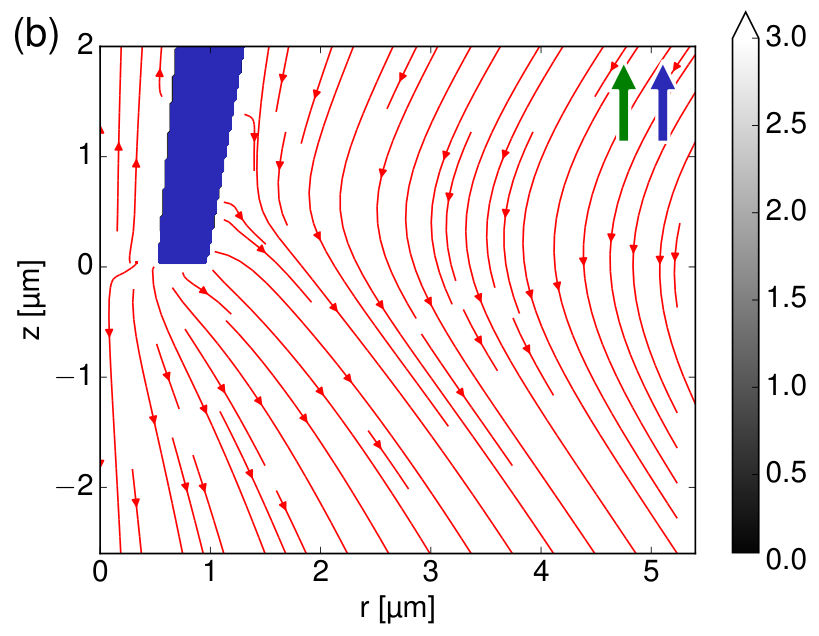
Figure 3a shows a small subvolume of the simulation domain at the tip of the capillary for the system with the aforementioned optimized parameters. The blue area represents the tapered capillary tip, the red streamlines depict the trajectories of a small charged particle with the above mobility $\mu$. The trajectories were obtained using the equation of motion (Eq. 1), with the electric field and flow profile from the FEM simulation as input. The green and blue arrows denote the direction of the pressure-driven flow and the EOF on the inside of the capillary, respectively.

Note that with the low salt concentrations and complex geometry used here, the interplay between the ionic distributions, electrostatics, and hydrodynamics can lead to unexpected polarization effects and even reversal of the EOF in the reservoir. [13]

The shape of the trajectories clearly shows transport of analyte molecules from the reservoir bulk to the capillary tip and a region directly at and in front of the capillary orifice, where they continuously recirculate. This effect directly corresponds to strong accumulation of highly concentrated DNA observed in the experiment (Fig. 2a).

Interestingly, the complicated interplay of EOF, pressure-driven flow, and electrophoresis does not lead to a simple stalling of analyte molecules at the capillary tip. Previous investigations based on one-dimensional transition state theory as carried out by Hoogerheide et al. [28] for solid state nanopores can therefore not be applied to this capillary based system. White et al. [14, 15, 16] have carried out studies using FEM based models similar to the one presented here. They investigated the nanopore translocation of a colloidal particle explicitly represented in the FEM simulation. They relied on the cylindrical symmetry of the system and could therefore not study the off-axis dynamics of the colloidal particle. Tsutsui et al. [29] investigated the off-axis translocation of a colloid through a solid-state nanopore and found significant differences to the on-axis translocation.

The gray-shaded background depicts the distance an analyte particle travels from a given point. The motion of particles in the recirculation region is limited to distances smaller than this trapping region. Consequently, the trapping region is shaded in black/dark-gray, according to its diameter of $1\text{\,}\mathrm{\SIUnitSymbolMicro m}2\text{\,}\mathrm{\SIUnitSymbolMicro m}$. The region shaded in lighter gray marks the subvolume from which analyte particles are transported into the trapping region. This capture region extends over $33\text{\,}\mathrm{\SIUnitSymbolMicro m}$ in the negative z-direction, all the way to the boundary of the simulation domain. Even at that boundary, the analyte molecules’ velocities due to advection and electrophoresis range from $1\text{\,}\mathrm{\SIUnitSymbolMicro m}2.5\text{\,}\mathrm{\SIUnitSymbolMicro m}$, significantly above the average thermal velocity of λ-phage DNA of $0.57\text{\,}\mathrm{\SIUnitSymbolMicro m}$. Analyte molecules originating in the white sub-volume do not become trapped: those molecules initially located more than $0.4\text{\,}\mathrm{\SIUnitSymbolMicro m}$ deep inside the capillary tip move up into the capillary, while particles located in the white region on the outside of the capillary move up along the outer capillary surface.
The size and position of the simulated trapping region in the left panel of Fig. 3a differs from that of the experimentally observed λ-phage DNA accumulation. The reasons for this are two-fold. Firstly, the optimized trapping parameters determined here do differ somewhat from the experimentally used parameters: the salt concentration is lower ($1\text{\,}\mathrm{mM}$ instead of $10\text{\,}\mathrm{mM}$), the applied voltage higher ($1\text{\,}\mathrm{V}$ instead of $500\text{\,}\mathrm{mV}$), and the pore orifice diameter smaller ($1\text{\,}\mathrm{\SIUnitSymbolMicro m}$ instead of $4\text{\,}\mathrm{\SIUnitSymbolMicro m}$). Such a change in the parameters to achieve trapping is expected, due to the relative physical simplicity of our model. Secondly, the simulation neglects the repulsive electrostatic and excluded volume interactions between different DNA molecules as discussed in Section II. The lack of repulsive interactions and the smaller orifice radius explain why the size of the trapping region in the simulations is smaller than that of the DNA accumulation observed in the experiment (Fig. 2a).

Figure 3b depicts the system with reversed voltage ($U=$-1\text{\,}\mathrm{V}$$) and otherwise identical parameters. The trajectories split up into two populations from where they were previously recirculating. One part of the molecules, which were previously trapped, now moves up into the capillary, while the other part disperses back into the reservoir. This situation also directly corresponds to the experimental observations as depicted in Fig. 2b. We therefore conclude that our simulation model accurately captures the relevant physics of the experimental system observed and described in Section III.1.

Having identified a set of parameters for this microcapillary based DNA trap, we now perform a numerical, exploratory study to determine whether this system can be tuned to trap a wide range of very specific molecules. We restrict ourselves to a numerical study here, as this is the most suited to consider a large parameter space and affords the most control over the variation of external parameters. While the fabrication method for the capillaries is relatively inexpensive and facile, performing a multitude of experiments on different types of molecules and varying external parameters is time consuming and costly, thus going well beyond the scope of the current work.
To determine the generality of capillary trapping, we varied the system parameters for the voltage, the pressure difference, the salt concentration, and the capillary surface charge, starting from the optimized parameters identified in Section III.2. For each of these systems, we then investigated the resulting trajectory field for its suitability as a trap, depending on the electrophoretic mobility of analyte molecules. This procedure yields upper and lower bounds for the trapping mobility of analyte molecules as a function of the varied system parameters. We refer to lower and higher mobilities in terms of their absolute values, that is, higher mobilities are more negative, while lower mobilities are mobilities closer to zero.
As Fig. 4 demonstrates, only particles with negative mobilities become trapped for all of the investigated parameters. Due to symmetry, positive analyte molecules can be trapped by applying the opposite pressure and voltage to a device of the same geometry but with opposite capillary surface charge.

Fig. 4a shows how the mobilities of trapped analyte particles vary with the salt concentration. We find that at low salt concentrations of $0.1\text{\,}\mathrm{mM}$, a relatively wide range of mobilities between $-1.08\text{\times}{10}^{-3}\text{\,}{\mathrm{cm}}^{2}\text{\,}{\mathrm{V}}^{-1}\text{\,}{\mathrm{s}}^{-1}$ and $-1.64\text{\times}{10}^{-3}\text{\,}{\mathrm{cm}}^{2}\text{\,}{\mathrm{V}}^{-1}\text{\,}{\mathrm{s}}^{-1}$ leads to trapping. Moderately increasing the salt concentration to $3\text{\,}\mathrm{mM}$ gradually shifts the interval for the mobilities of trapped particles to lower values and continuously increases the specificity of the trap. At a salt concentration of $3\text{\,}\mathrm{mM}$, only particles with mobilities in the range from $-6.90\text{\times}{10}^{-4}\text{\,}{\mathrm{cm}}^{2}\text{\,}{\mathrm{V}}^{-1}\text{\,}{\mathrm{s}}^{-1}$ to $-7.09\text{\times}{10}^{-4}\text{\,}{\mathrm{cm}}^{2}\text{\,}{\mathrm{V}}^{-1}\text{\,}{\mathrm{s}}^{-1}$ become trapped. Experimentally varying the salt concentration within this range from $0.1\text{\,}\mathrm{mM}$ to $3\text{\,}\mathrm{mM}$ is very feasible.
Fig. 4b shows the range of mobilities of trapped particles as a function of the capillary surface charge density. Varying the pore surface charge density from $-0.07\text{\,}\mathrm{C}\text{\,}\mathrm{m}-0.01\text{\,}\mathrm{C}\text{\,}\mathrm{m}$ allows us to tune the mobilities of trapped particles to very similar bounds as before when varying the salt concentration from $0.1\text{\,}\mathrm{mM}$ to $3\text{\,}\mathrm{mM}$. At a surface charge concentration of $-0.07\text{\,}\mathrm{C}\text{\,}\mathrm{m}$, analyte particles with mobilities in the range from $-1.31\text{\times}{10}^{-3}\text{\,}{\mathrm{cm}}^{2}\text{\,}{\mathrm{V}}^{-1}\text{\,}{\mathrm{s}}^{-1}$ to $-1.75\text{\times}{10}^{-3}\text{\,}{\mathrm{cm}}^{2}\text{\,}{\mathrm{V}}^{-1}\text{\,}{\mathrm{s}}^{-1}$ become trapped. With decreasing capillary surface charge density (in absolutes), this interval gradually moves to lower mobilities and the trap becomes more specific. At a capillary surface charge density of $-0.01\text{\,}\mathrm{C}\text{\,}{\mathrm{m}}^{-1}$, only particles with mobilities in the range from $-5.97\text{\times}{10}^{-4}\text{\,}{\mathrm{cm}}^{2}\text{\,}{\mathrm{V}}^{-1}\text{\,}{\mathrm{s}}^{-1}$ to $-6.71\text{\times}{10}^{-4}\text{\,}{\mathrm{cm}}^{2}\text{\,}{\mathrm{V}}^{-1}\text{\,}{\mathrm{s}}^{-1}$ become trapped. This range includes the mobility of λ-phage DNA $\mu_{\text{DNA}}=$-6.23\text{\times}{10}^{-4}\text{\,}{\mathrm{cm}}^{2}\text{\,}{\mathrm{V}}^{-1}\text{\,}{\mathrm{s}}^{-1}$$ at $1\text{\,}\mathrm{mM}$ salt concentration. [27] Varying the spatial distribution of the capillary surface charge density experimentally is non-trivial. However, surface charge can be controlled changing the pH, or by using a wide range of available polyelectrolyte coatings, or even coatings with lipid membranes. All of these surface coatings can suppress or enhance EOF, leading to an effective surface charge that can be tuned over a wide range.
Fig. 4c depicts the dependency of the trapped particle’s mobility as a function of the applied voltage. We vary the applied voltage from $0.8\text{\,}\mathrm{V}1.6\text{\,}\mathrm{V}$ and find that in contrast with the other parameters, the voltage in this range does not change the specificity of the trap drastically. At $0.8\text{\,}\mathrm{V}$, particles with mobilities between $-8.21\text{\times}{10}^{-4}\text{\,}{\mathrm{cm}}^{2}\text{\,}{\mathrm{V}}^{-1}\text{\,}{\mathrm{s}}^{-1}$ and $-9.70\text{\times}{10}^{-4}\text{\,}{\mathrm{cm}}^{2}\text{\,}{\mathrm{V}}^{-1}\text{\,}{\mathrm{s}}^{-1}$ become trapped. With increasing voltage, this interval moves to higher mobilities. At $1.6\text{\,}\mathrm{V}$, particles with mobilities between $-9.32\text{\times}{10}^{-4}\text{\,}{\mathrm{cm}}^{2}\text{\,}{\mathrm{V}}^{-1}\text{\,}{\mathrm{s}}^{-1}$ and $-1.27\text{\times}{10}^{-3}\text{\,}{\mathrm{cm}}^{2}\text{\,}{\mathrm{V}}^{-1}\text{\,}{\mathrm{s}}^{-1}$ become trapped. Electrolysis of water happens for voltages exceeding $1.23\text{\,}\mathrm{V}$, negatively impacting the experiment due to pH shifts and bubble formation at the electrodes causing current instabilities. [30]
Finally, Fig. 4d shows how the applied pressure difference influences the mobilities of trapped particles. The lower limit for the mobility of trapped particles is only weakly affected by varying the pressure difference in the range from $-400\text{\,}\mathrm{Pa}-150\text{\,}\mathrm{Pa}$ and varies from $-8.21\text{\times}{10}^{-4}\text{\,}{\mathrm{cm}}^{2}\text{\,}{\mathrm{V}}^{-1}\text{\,}{\mathrm{s}}^{-1}$ to $-8.58\text{\times}{10}^{-4}\text{\,}{\mathrm{cm}}^{2}\text{\,}{\mathrm{V}}^{-1}\text{\,}{\mathrm{s}}^{-1}$. The upper limit of mobilities leading to trapping, on the other hand, is significantly affected by that change in pressure and changes from $-8.58\text{\times}{10}^{-4}\text{\,}{\mathrm{cm}}^{2}\text{\,}{\mathrm{V}}^{-1}\text{\,}{\mathrm{s}}^{-1}$ at a pressure of $-400\text{\,}\mathrm{Pa}$ to $-1.27\text{\times}{10}^{-3}\text{\,}{\mathrm{cm}}^{2}\text{\,}{\mathrm{V}}^{-1}\text{\,}{\mathrm{s}}^{-1}$ at a pressure of $-150\text{\,}\mathrm{Pa}$. These pressure differences can easily be achieved experimentally by closing the reservoirs and connecting them to a microfluidic pressure regulator.
Our results in Fig. 4 therefore suggest that varying the salt concentration or the pore surface charge density within experimentally plausible values offers the greatest specificity for trapping analyte molecules. Pressure variations in the region of $-400\text{\,}\mathrm{Pa}-350\text{\,}\mathrm{Pa}$ also offer a reasonable degree of specificity, but varying the voltage has little effect on specificity. This is in a sense fortuitous since voltages exceeding $1.23\text{\,}\mathrm{V}$ cause the undesirable electrolysis of water. Our glass nanopore system therefore shows strong promise as an experimental useful and cheap system for trapping charged macromolecules with a high degree of control.

References

- [1] A. J. Ninfa, D. P. Ballou, and M. Benore, Fundamental Laboratory Approaches for Biochemistry and Biotechnology (Wiley, 2009).
- [2] P. Cuatrecasas, J. Biol. Chem. 245, 3059 (1970).
- [3] D. Figeys and D. Pinto, Anal. Chem. 72, 330 A (2000).
- [4] C. L. Asbury and G. v. d. Engh, Biophysical Journal 74, 1024 (1998).
- [5] C. L. Asbury, A. H. Diercks, and G. van den Engh, Electrophoresis 23, 2658 (2002).
- [6] Y.-C. Wang, A. L. Stevens, and J. Han, Anal. Chem. 77, 4293 (2005).
- [7] Z. Huang and C. F. Ivory, Anal. Chem. 71, 1628 (1999).
- [8] D. Stein, Z. Deurvorst, F. H. J. van der Heyden, W. J. A. Koopmans, A. Gabel, and C. Dekker, Nano Lett. 10, 765 (2010).
- [9] L. Ying, A. Bruckbauer, A. M. Rothery, Y. E. Korchev, and D. Klenerman, Anal. Chem. 74, 1380 (2002).
- [10] L. Ying, S. S. White, A. Bruckbauer, L. Meadows, Y. E. Korchev, and D. Klenerman, Biophysical Journal 86, 1018 (2004).
- [11] H. S. White and A. Bund, Langmuir 24, 2212 (2008).
- [12] N. Laohakunakorn and U. F. Keyser, Nanotechnology 26, 275202 (2015).
- [13] N. Laohakunakorn, V. V. Thacker, M. Muthukumar, and U. F. Keyser, Nano Lett. 15, 695 (2015).
- [14] W.-J. Lan, D. A. Holden, B. Zhang, and H. S. White, Anal. Chem. 83, 3840 (2011).
- [15] S. R. German, L. Luo, H. S. White, and T. L. Mega, J. Phys. Chem. C 117, 703 (2013).
- [16] W.-J. Lan, C. Kubeil, J.-W. Xiong, A. Bund, and H. S. White, J. Phys. Chem. C 118, 2726 (2014).
- [17] N. Laohakunakorn, S. Ghosal, O. Otto, K. Misiunas, and U. F. Keyser, Nano Lett. 13, 2798 (2013).
- [18] M. Mao, S. Ghosal, and G. Hu, Nanotechnology 24, 245202 (2013).
- [19] V. V. Thacker, S. Ghosal, S. Hernández-Ainsa, N. A. W. Bell, and U. F. Keyser, Appl. Phys. Lett. 101, 223704 (2012).
- [20] G. S. Manning, J. Phys. Chem. 85, 1506 (1981).
- [21] E. Hückel, Phys. Z 25, 204 (1924).
- [22] M. v. Smoluchowski, Bull. Int. Acad. Sci. Cracovie , 182 (1903).
- [23] R. W. O’Brien and L. R. White, J. Chem. Soc. Farad. T. 2 74, 1607 (1978).
- [24] N. C. Stellwagen, C. Gelfi, and P. G. Righetti, Biopolymers 42, 687 (1997).
- [25] S. Allison, C. Chen, and D. Stigter, Biophys. J. 81, 2558 (2001).
- [26] G. Rempfer, G. B. Davies, C. Holm, and J. de Graaf, arXiv:1604.02054 [cond-mat] (2016).
- [27] D. A. Hoagland, E. Arvanitidou, and C. Welch, Macromolecules 32, 6180 (1999).
- [28] D. P. Hoogerheide, B. Lu, and J. A. Golovchenko, ACS Nano 8, 7384 (2014).
- [29] M. Tsutsui, Y. He, K. Yokota, A. Arima, S. Hongo, M. Taniguchi, T. Washio, and T. Kawai, ACS Nano 10, 803 (2016).
- [30] P. Atkins and J. d. Paula, Elements of Physical Chemistry (OUP Oxford, 2013).