∎

Quantum Image Matching Thanks: This work is supported by the National Natural Science Foundation of China under Grants No. 61502016, the Fundamental Research Funds for the Central Universities under Grants No. 2015JBM027, and the Graduate Technology Fund of BJUT under Grants No. ykj-2015-11719.

Nan Jiang Yijie Dang Jian Wang Affiliation: College of Computer Science, Beijing University of Technology, Beijing 100124, China
College of Science, Purdue University, West Lafayette 47905, USA
Beijing Key Laboratory of Trusted Computing, Beijing 100124, China
National Engineering Laboratory for Critical Technologies of Information Security Classified Protection, Beijing 100124, China Affiliation: College of Computer Science, Beijing University of Technology, Beijing 100124, China Affiliation: School of Computer and Information Technology, Beijing Jiaotong University, Beijing 100044, China
College of Science, Purdue University, West Lafayette 47905, USA E-mail: wangjian@bjtu.edu.cn

Received: date / Accepted: date

Abstract

Quantum image processing (QIP) means the quantum based methods to speed up image processing algorithms. Many quantum image processing schemes claim that their efficiency are theoretically higher than their corresponding classical schemes. However, most of them do not consider the problem of measurement. As we all know, measurement will lead to collapse. That is to say, executing the algorithm once, users can only measure the final state one time. Therefore, if users want to regain the results (the processed images), they must execute the algorithms many times and then measure the final state many times to get all the pixels’ values. If the measurement process is taken into account, whether or not the algorithms are really efficient needs to be reconsidered. In this paper, we try to solve the problem of measurement and give a quantum image matching algorithm. Unlike most of the QIP algorithms, our scheme interests only one pixel (the target pixel) instead of the whole image. It modifies the probability of pixels based on Grover’s algorithm to make the target pixel to be measured with higher probability, and the measurement step is executed only once. An example is given to explain the algorithm more vividly. Complexity analysis indicates that the quantum scheme’s complexity is $O(2^{n})$ in contradistinction to the classical scheme’s complexity $O(2^{2n+2m})$ , where $m$ and $n$ are integers related to the size of images.

Keywords:

Quantum image processing Quantum computation Quantum image matching

1 Introduction

In 1982, Feynman proposed a novel computation model, named quantum computers which can efficiently solve some problems that are believed to be intractable on classical computers [1]. After that, many researchers devote themselves into the research about quantum computers. The latest research shows that quantum computers are 100 million times faster than classical computers [2].

The developing of quantum computer causes people’s interest to study quantum image processing (QIP) which refers to use quantum computers to process images. Many researchers have proposed a number kinds of QIP algorithms, such as geometric transformation [3-6], color transformation [7-8], image scrambling [9-11], image segmentation [12-14], feature extraction [15], quantum image watermark [16-23], quantum image encryption [24-27], and quantum imaging [32]. Their efficiency are theoretically higher than their corresponding classical schemes.

However, most of them do not consider the problem of measurement. Fig. 1(a) gives an example.

Refer to caption — Figure 1: The difference between ordinary quantum image processing algorithms and our scheme.

No matter the image are the original one or the processed one, its representation method is similar: a superposition state is used to store the image and every pixel has the same probability to be measured. Taking the processed image in Fig. 1(a) as an example, its representation is

|I\rangle=\frac{1}{2}|1101\rangle\otimes|00\rangle+\frac{1}{2}|1111\rangle\otimes|01\rangle+\frac{1}{2}|1100\rangle\otimes|10\rangle+\frac{1}{2}|1011\rangle\otimes|11\rangle.

$|I\rangle$ is a superposition state. If we want to read the image out, it must be measured. However, once the state is measured, it will collapse to the non-superposition state that has been measured. That is to say, once a pixel is measured, other pixels will disappear. Like the image $|I\rangle$ , it has 4 pixels and the probabilities of a pixel being measured are all $\left(\frac{1}{2}\right)^{2}=\frac{1}{4}$ . If the pixel being measured is $|1111\rangle\otimes|01\rangle$ , $|I\rangle$ collapses to $|1111\rangle\otimes|01\rangle$ and the other 3 pixels disappear. How to measure the other pixels? The only method is performing the quantum image processing again. Most fortunately, if a different pixel is measured each time, by repeating the whole process 4 times, the 4 pixels’ values are regained. However, if we are not so fortunate, it can not say the exact number of repetitions, maybe 10 times, maybe 100 times, and maybe never get all the 4 values.

Hence, in order to read out the result, users must execute the quantum algorithm many times. Therefore, whether or not the algorithms are really efficient needs to be reconsidered. In Ref. [38-39], Mario Mastriani holds a similar view.

In this paper, we try to solve the problem of measurement and give a quantum image matching algorithm (see Fig. 1(b)). This scheme modifies the probability of pixels to make the target pixel to be measured with higher probability and the whole scheme is executed only once.

The rest of the paper is organized as follows. Sect. 2 gives related works about quantum image matching. Sect. 3 introduces what image matching is. Our scheme is discussed in Sect. 4 including the basic ideas, the scheme steps, and the theoretical analysis. Sect. 5 analysis the network complexity. Sect. 6 gives the conclusion.

2 Related works

There have been several references that discuss the quantum image matching.

Yang and etc give a quantum gray-scale image matching scheme in Ref. [34], in which the quantum template image is directly mapped with quantum reference image, i.e., the quantum register representing each corresponding pixel of the quantum template image is subtracted from that of the quantum reference image by running a quantum subtracter. According to the quantum measurement results, the difference is saved and sum all the differences. Then compare the sum with a Tolerance value. If the sum is smaller than the Tolerance value, then quantum image matching succeeds. However, we think that it has 3 shortcomings: (1) Although the title is “quantum image matching”, in fact, the paper computes the similarity between two quantum images instead of giving a quantum image matching scheme. (2) What the quantum part of the scheme does only is subtraction, which can be done more efficiently in classical computers. (3) It needs to regain all the pixels in the different image, i.e., it needs to be processed and measured many times.

A chaotic quantum-behaved particle swarm optimization based on lateral inhibition (LI-CQPSO) is proposed in Ref. [35], which is used to solve complicated image matching problems. In this work, the proposed LI-CQPSO combines the techniques of chaos theory, quantum and lateral inhibition. Chaos can guarantee the PSO escaping from local best, quantum can make the traditional PSO with better searching performance as well as having fewer parameters to control, and lateral inhibition is applied to extract the edge of the images by sharpening the spatial profile of excitation in response to a localized stimulus. However, it is a classical algorithm and all steps are done in classical computers. Quantum-behaved particle swarm optimization (QPSO) is only motivated by concepts from quantum mechanics, but is not a quantum algorithm.

Ref. [36] proposes to combine the shape context (SC) descriptor with quantum genetic algorithms (QGA) to define a new shape matching and retrieval method. The SC matching method is based on finding the best correspondence between two point sets. However, it is suitable for shape matching instead of natural images matching.

The algorithm proposed in Ref. [37] is similar to our work: change the probability of the target pixel. However, as the authors say in this paper, it is not a complete solution because that although the probability of the target pixel is larger than the probability of other pixels, it is still relatively small.

Unlike the above works, we will give a quantum image matching solution which does not compute similarity, is not a classical algorithm based on quantum concepts, and is not for shape matching.

3 Image matching

Image matching is the process of searching for a small image in a big image. It is widely used in computer vision, military automatic target recognition, face detection, manufacturing quality control, visual positioning and tracking, and so on. Fig. 2 gives an example.

The simplest image matching method is the exhaustive search. Assume that the size of the big image is $2^{n}\times 2^{n}$ and the size of the small image is $2^{m}\times 2^{m}$ , where $n>m$ . For each $2^{m}\times 2^{m}$ image block in the big image, the method compares all the pixels in the block with the corresponding ones in the small image. If the block is the same as the small image, the method will finish its work and output the block’s location. Hence, the complexity of the exhaustive search is $O(2^{2n+2m})$ . It is exponential and too high to bear in most application cases.

Therefore, researchers give other schemes to reduce the complexity. Most of them take advantage of the features of images:

$\bullet$

Feature-based scheme compares the image features instead of the whole image pixels to match two images [28]. Color, edge, feature points and so on can all be used as features. Fig. 3 gives two examples. In general, no matter what kind of features, their data volume is obviously smaller than the original image (the pixels), which helps to reduce the complexity.

(a) Feature points (Only the red points are feature points.)

(b) Edge

Figure 3: Different kinds of features.
$\bullet$

Frequency-domain schemes find the transformation parameters for matching [29]. The commonly used transformations include the discrete cosine transform, the discrete Fourier transform, the discrete wavelet transform and so on. This method can not only reduce the complexity by cutting down the data volume to be compared, but also tolerate a certain degree of deformation caused by illumination, angle, distance and etc (see Fig. 4).

(a) illumination

(b) angle

(c) distance

Figure 4: Deformation caused by illumination, angle and distance, in which (a) and (b) are cited from [30].
$\bullet$

Interactive schemes provide tools to match the images manually which reduce user bias by performing certain key operations automatically while still relying on the user to guide the matching [29].

Although these improved schemes enhance the performance of image matching, it is still a difficult problem in image processing because the efficiency is unsatisfactory yet.

In this paper, by taking advantage of the high computing ability of quantum computers, we give a quantum image matching algorithm to reduce the complexity.

4 Quantum image matching algorithm

4.1 Basic ideas

We use the generalized quantum image representation (GQIR) method [6] to store quantum images in this paper. GQIR is developed from the novel enhanced quantum representation (NEQR) [7] with the difference that GQIR can represent arbitrary $H\times W$ images instead of only $2^{n}\times 2^{n}$ images. If a quantum image is with size $2^{n}\times 2^{n}$ , its GQIR representation and NEQR representation are the same. Readers please refer Ref. [6] about GQIR’s preparation and analysis. For the sake of simplicity, in this paper, we only describe GQIR briefly.

An images can be seen as a function: $I(x,y)$ . Hence, a GQIR image is represented as an entangled state

|I(x,y)\rangle\otimes|xy\rangle

(1)

Assume that the size of an image is $2^{n}\times 2^{n}$ and $I(x,y)\in\{0,1,\cdots,2^{q}-1\}$ . Due to the equal role of every pixels in an image, their probability are equivalent. Hence,

|xy\rangle=\frac{1}{\sqrt{2^{2n}}}\sum_{k=0}^{2^{2n}-1}|k\rangle=\frac{1}{2^{n}}\sum_{k=0}^{2^{2n}-1}|k\rangle

(2)

In image matching, the inputs are two images: the big image $A$ with size $2^{n}\times 2^{n}$ and the small image $B$ with size $2^{m}\times 2^{m}$ , where $n>m$ . The matching algorithm’s output is the location $(x,y)$ of the upper left pixel of $B$ in $A$ . Fig. 5 gives a sketch map.

In order to get $(x,y)$ in measurement, the basic idea of our solution is to increase the probability of $(x,y)$ and reduce the probability of other pixels. As early as 1996, Grover had provided the idea [31]. In this paper, we use it into quantum image matching.

4.2 Algorithm

According to the previous presentation, the two input images $A$ and $B$ are

|A\rangle=\frac{1}{2^{n}}\sum_{k_{A}=0}^{2^{2n}-1}|I_{A}(k_{A})\rangle\otimes|k_{A}\rangle

(3)

|B\rangle=\frac{1}{2^{m}}\sum_{k_{B}=0}^{2^{2m}-1}|I_{B}(k_{B})\rangle\otimes|k_{B}\rangle

(4)

Additionally, two auxiliary qubit $|f\rangle=|0\rangle$ and $|g\rangle=\frac{1}{\sqrt{2}}(|0\rangle-|1\rangle)$ are needed. Hence, the initial state of the algorithm is

\begin{split}\Psi_{0}&=|g\rangle\otimes|f\rangle\otimes|A\rangle\otimes|B\rangle\\ &=|g\rangle\otimes\left(\frac{1}{2^{n+m}}\sum_{k_{A}=0}^{2^{2n}-1}\sum_{k_{B}=0}^{2^{2m}-1}|0\rangle\otimes|I_{A}(k_{A})\rangle\otimes|k_{A}\rangle\otimes|I_{B}(k_{B})\rangle\otimes|k_{B}\rangle\right)\end{split}

(5)

Step 1

Find out the matched area, i.e., the pixels that $I_{A}=I_{B}$ .

Due to $I_{A},I_{B}\in\{0,1,\cdots,2^{q}-1\}$ , $q$ qubits are used to store $|I_{A}\rangle$ and $|I_{B}\rangle$ .

|I_{T}(k_{T})\rangle=|I^{q-1}_{T}(k_{T})I^{q-2}_{T}(k_{T})\cdots I^{0}_{T}(k_{T})\rangle

(6)

where, $T\in\{A,B\}$ and $I^{i}_{T}(k_{T})\in\{0,1\}$ , $i=q-1,q-2,\cdots,0$ .

Define

U_{1}^{i}:|I^{i}_{A},I^{i}_{B}\rangle\rightarrow|I^{i}_{A}\oplus I^{i}_{B},I^{i}_{B}\rangle

(7)

That is to say, $U_{1}^{i}$ is a CNOT gate: if $I^{i}_{A}=I^{i}_{B}$ , $I^{i}_{A}$ is changed to 0; otherwise, $I^{i}_{A}$ is changed to 1. Hence, by acting

U_{1}=\bigotimes_{i=q-1}^{0}U_{1}^{i}

(8)

to state $\Psi_{0}$ , we can get

\begin{split}\Psi_{1}&=U_{1}(\Psi_{0})\\ &=|g\rangle\otimes\left(\frac{1}{2^{n+m}}\sum_{k_{A}}\sum_{k_{B}}|0\rangle\otimes[\otimes_{i=q-1}^{0}|I^{i}_{A}(k_{A})\oplus I^{i}_{B}(k_{B})\rangle]\otimes|k_{A}\rangle\otimes|I_{B}(k_{B})\rangle\otimes|k_{B}\rangle\right)\\ &=|g\rangle\otimes\left(\frac{1}{2^{n+m}}\sum_{k_{A}}\sum_{k_{B}}|0\rangle\otimes|I_{A}(k_{A})\oplus I_{B}(k_{B})\rangle\otimes|k_{A}\rangle\otimes|I_{B}(k_{B})\rangle\otimes|k_{B}\rangle\right)\end{split}

(9)

For the sake of simplicity, when no ambiguity is possible, we still use $I_{A}(k_{A})$ to substitute $I_{A}(k_{A})\oplus I_{B}(k_{B})$ . Therefore

\begin{split}\Psi_{1}=&|g\rangle\otimes\left(\frac{1}{2^{n+m}}\sum_{k_{A}}\sum_{k_{B}}|0\rangle\otimes|I_{A}(k_{A})\rangle\otimes|k_{A}\rangle\otimes|I_{B}(k_{B})\rangle\otimes|k_{B}\rangle\right)\\ =&|g\rangle\otimes\left(\frac{1}{2^{n+m}}\left[\sum_{k_{A},k_{B},\text{ and }I_{A}=I_{B}}|0\rangle\otimes|0\rangle^{\otimes q}\otimes|k_{A}\rangle\otimes|I_{B}(k_{B})\rangle\otimes|k_{B}\rangle\right.\right.\\ &\left.\left.+\sum_{k_{A},k_{B},\text{ and }I_{A}\neq I_{B}}|0\rangle\otimes|I_{A}(k_{A})\rangle\otimes|k_{A}\rangle\otimes|I_{B}(k_{B})\rangle\otimes|k_{B}\rangle\right]\right)\end{split}

(10)

Therefore, in image $A$ , all the pixels that $I_{A}=I_{B}$ , i.e., in state $\Psi_{1}$ , all the pixels that $|I_{A}\rangle=|0\rangle^{\otimes q}$ , consist the matched area.

Step 2

Find out the upper left corner of the matched area.

Although the matched area is found out, the upper left corner of it is still unknown. However, in image $B$ , the upper left corner is fixed: it is pixel $(0,0)$ . Hence, in $\Psi_{1}=|g\rangle\otimes\left(\frac{1}{2^{n+m}}\sum_{k_{A}}\sum_{k_{B}}|0\rangle\otimes|I_{A}(k_{A})\rangle\otimes|k_{A}\rangle\otimes|I_{B}(k_{B})\rangle\otimes|k_{B}\rangle\right)$ , when $|I_{A}(k_{A})\rangle=|0\rangle^{\otimes q}$ and $|k_{B}\rangle=|0\rangle^{\otimes m}$ , their corresponding $|k_{A}\rangle$ is the quantum image matching algorithm’s output. We call it as $|k_{A_{0}}\rangle$ . In Step 2, a transform $U_{2}$ is used to change the state of the auxiliary qubit $|f\rangle$ .

U_{2}:|f=0\rangle\rightarrow|f=1\rangle\text{, if }|I_{A}(k_{A})\rangle=|0\rangle^{\otimes q}\text{ and }|k_{B}\rangle=|0\rangle^{\otimes m}

(11)

where, $U_{2}$ is a $(q+m)$ -CNOT gate (a CNOT gate with $(q+m)$ control qubits).

Act $U_{2}$ to $\Psi_{1}$

\begin{split}\Psi_{2}=&U_{2}(\Psi_{1})\\ =&|g\rangle\otimes\left(\frac{1}{2^{n+m}}\left[|1\rangle\otimes|0\rangle^{\otimes q}\otimes|k_{A_{0}}\rangle\otimes|I_{B}(k_{B})\rangle\otimes|0\rangle^{\otimes 2m}\right.\right.\\ &\left.\left.+\sum_{I_{A}\neq|0\rangle^{\otimes q}\text{ or }|k_{B}\rangle\neq|0\rangle^{\otimes m}}|0\rangle\otimes|I_{A}(k_{A})\rangle\otimes|k_{A}\rangle\otimes|I_{B}(k_{B})\rangle\otimes|k_{B}\rangle\right]\right)\end{split}

(12)

That is to say, in the superposition state $\Psi_{2}$ , the basis that $|f\rangle=|1\rangle$ corresponds to the upper left corner of the matched area.

Step 3

Change the probability of subspace $|k_{A}\rangle$ .

In the first two steps, the upper left corner of the matched area has been found out according to the color information $|I_{A}\rangle$ and $|I_{B}\rangle$ and location information $|k_{B}\rangle$ . $|f\rangle$ is the deliverable of the first two steps. Hence, The three information ( $|I_{A}\rangle$ , $|I_{B}\rangle$ and $|k_{B}\rangle$ ) has no use in the following and $|f\rangle$ substitutes them.

Therefore, in this step, we only work on the subspace $|k_{A}\rangle$ and increase the probability of $|k_{A_{0}}\rangle$ based on Grover’s algorithm. Hence, the initial state of Step 3 is

\begin{split}\Psi_{30}=&|k_{A}\rangle\otimes|g\rangle\otimes|f\rangle\\ =&\frac{1}{2^{n}\sqrt{2}}\left[|k_{A_{0}}\rangle\otimes(|0\rangle-|1\rangle)\otimes|1\rangle+\sum_{f=0}|k_{A}\rangle\otimes(|0\rangle-|1\rangle)\otimes|f\rangle\right]\end{split}

(13)

Step 3.1

Rotate the phase of $|k_{A_{0}}\rangle$ by $\pi$ radians with the help of the auxiliary qubit $|g\rangle$ [33].

Define

U_{31}:|k_{A},g,f\rangle\rightarrow|k_{A},g\oplus f,f\rangle

(14)

Obviously, $U_{31}$ is a CNOT gate. Then

\begin{split}\Psi_{31}=&U_{31}(\Psi_{30})\\ =&\frac{1}{2^{n}\sqrt{2}}\left[|k_{A_{0}}\rangle\otimes(|1\rangle-|0\rangle)\otimes|1\rangle+\sum_{f=0}|k_{A}\rangle\otimes(|0\rangle-|1\rangle)\otimes|f\rangle\right]\\ =&-\frac{1}{2^{n}}|k_{A_{0}}\rangle\otimes|g\rangle\otimes|f\rangle+\frac{1}{2^{n}}\sum_{f=0}|k_{A}\rangle\otimes|g\rangle\otimes|f\rangle\end{split}

(15)

Hence, in the subspace $|k_{A}\rangle$ ,

\Psi_{31}=\left(\frac{1}{2^{n}},\cdots,\frac{1}{2^{n}},-\frac{1}{2^{n}},\frac{1}{2^{n}},\cdots,\frac{1}{2^{n}}\right)^{\text{T}}

(16)

That is to say, the function of Step 3.1 is to change the coefficient of $k_{A_{0}}$ to a negative.

Step 3.2

Increase the probability of $|k_{A_{0}}\rangle$ and decrease the probability of other $|k_{A}\rangle$ .

Apply the diffusion transform $D$ on $\Psi_{31}$ which is defined by the matrix $D$ as follows [31]:

$D_{ij}=\frac{2}{2^{2n}}\text{ if }i\neq j,\text{ and }D_{ii}=\frac{2}{2^{2n}}-1$ (17)

This diffusion transform $D$ can be implemented as $D=WRW$ , where $R$ is the rotation matrix and $W$ is the Walsh-Hadamard Transform Matrix are defined as follows:

$R_{ij}=0\text{ if }i\neq j,\text{ and }R_{00}=1,\text{ and }R_{ii}=-1\text{ if }i\neq 0$ (18)

$W_{ij}=\frac{1}{2^{n}}(-1)^{\overline{i}\cdot\overline{j}}$ (19)

where $\overline{i}$ is the binary representation of $i$ , and $\overline{i}\cdot\overline{j}$ denotes the bitwise dot product of the two strings $\overline{i}$ and $\overline{j}$ .

After Step 3.2, the probability of $|k_{A_{0}}\rangle$ is increased and the probability of other pixels is decreased.
Step 3.3

Repeat the unitary operations Step 3.1 and 3.2

$\hat{i}\approx 0.7962a-0.6057$ (20)

times, where $a=2^{n}$ (Eq. (20) will be proved in Section 4.3). In the subspace $|k_{A}\rangle$ , the final state of this step is

$\Psi_{33}=\left(t_{\hat{i}},\cdots,t_{\hat{i}},t_{\hat{i}0},t_{\hat{i}},\cdots,t_{\hat{i}}\right)^{\text{T}}$ (21)

where, $t_{\hat{i}0}$ is the corresponding element of $|k_{A_{0}}\rangle$ and $t_{\hat{i}}$ is the corresponding element of other pixels.

Step 4

Measurement.

Use projective measurements to measure state $\Psi_{33}$ and define measurement operators as

P_{j}=|j\rangle\langle j|,\ j=0,1,\cdots,2^{2n-1}

(22)

Hence, the probability that the basis $|j\rangle$ being measured is

\langle\Psi_{33}|P_{j}|\Psi_{33}\rangle=(t_{j})^{2}

(23)

where, $t_{j}$ is the $j$ th element in $\Psi_{33}$ , $j=0,1,\cdots,2^{2n-1}$ . Hence, the basis $|k_{A_{0}}\rangle$ (i.e., the upper left corner of the matched area) is measured with probability $t_{\hat{i}0}^{2}$ and

t_{\hat{i}0}^{2}\geq(0.9194+0.0567a^{-1}+0.2302a^{-2}-0.0336a^{-3})^{2}.

(24)

(Eq. (24) will be proved in Section 4.3)

Fig. 6 gives the circuit of quantum image matching.

4.3 Lemmas and theorems

In Section 4.2, there are two key variables: $\hat{i}$ and $t_{\hat{i}0}$ . In this section, we will prove their values, i.e., Eq. (20) and (24).

Lemma 1

The output of Step 3.2 after the $i$ th iteration is in the form of

T_{i}=\left(t_{i},\cdots,t_{i},t_{i0},t_{i},\cdots,t_{i}\right)^{\text{T}}

(25)

and

\begin{split}t_{(i+1)0}=&-\frac{2t_{i0}}{a^{2}}-\frac{2t_{i}}{a^{2}}+2t_{i}+t_{i0}\\ t_{i+1}=&-\frac{2t_{i0}}{a^{2}}-\frac{2t_{i}}{a^{2}}+t_{i}\end{split}

(26)

where $a=2^{n}$ . That is to say, after the $i$ th iteration, the output $T_{i}$ only has two values: $t_{i}$ and $t_{i0}$ and $t_{i0}^{2}$ is the probability of $|k_{A_{0}}\rangle$ being measured and $t_{i}^{2}$ is the probability of other $|k_{A}\rangle$ being measured.

Proof.

According to Eq. (17),

D\equiv-I+2P

(27)

where $I$ is the identity matrix and $P$ is a projection matrix with $P_{ij}=\frac{1}{2^{2n}}$ for all $i,j$ . Hence, for an arbitrary $2^{2n}\times 1$ matrix $S$

\begin{split}&DS=D\left(\begin{array}[]{c}s_{0}\\ s_{1}\\ \cdots\\ s_{2^{2n}-1}\\ \end{array}\right)=(2P-I)\left(\begin{array}[]{c}s_{0}\\ s_{1}\\ \cdots\\ s_{2^{2n}-1}\\ \end{array}\right)\\ =&\left(\begin{array}[]{c}2\cdot\frac{s_{0}+s_{1}+\cdots+s_{2^{2n}-1}}{2^{2n}}-s_{0}\\ 2\cdot\frac{s_{0}+s_{1}+\cdots+s_{2^{2n}-1}}{2^{2n}}-s_{1}\\ \cdots\\ 2\cdot\frac{s_{0}+s_{1}+\cdots+s_{2^{2n}-1}}{2^{2n}}-s_{2^{2n}-1}\\ \end{array}\right)=\left(\begin{array}[]{c}2\overline{s}-s_{0}\\ 2\overline{s}-s_{1}\\ \cdots\\ 2\overline{s}-s_{2^{2n}-1}\\ \end{array}\right)\end{split}

(28)

where $\overline{s}=\frac{s_{0}+s_{1}+\cdots+s_{2^{2n}-1}}{2^{2n}}$ is the average value of $s_{0},s_{1},\cdots,s_{2^{2n}-1}$ . From Eq. (28), it is obviously that if $s_{i}=s_{j}$ , then $2\overline{s}-s_{i}=2\overline{s}-s_{j}$ . Due to the input of Step 3.2 in the first iteration is $\Psi_{31}=\left(\frac{1}{2^{n}},\cdots,\frac{1}{2^{n}},-\frac{1}{2^{n}},\frac{1}{2^{n}},\cdots,\frac{1}{2^{n}}\right)^{\text{T}}$ which only has two values: $\frac{1}{2^{n}}$ and $-\frac{1}{2^{n}}$ , i.e., $t_{00}=t_{0}=\frac{1}{2^{n}}=\frac{1}{a}$ , hence

T_{1}=\left(t_{1},\cdots,t_{1},t_{10},t_{1},\cdots,t_{1}\right)^{\text{T}}

and if we use $\overline{t}_{i}$ to respect the average value in the $i$ th iteration,

\overline{t}_{1}=\left.\left((a^{2}-1)\cdot t_{0}-t_{00}\right)\middle/a^{2}\right.=\left.\left((a^{2}-1)\cdot\frac{1}{a}-\frac{1}{a}\right)\middle/a^{2}\right.=\frac{1}{a}-\frac{2}{a^{3}}

then

t_{10}=2\overline{t}_{1}+t_{00}=\frac{3}{a}-\frac{4}{a^{3}}=-\frac{2t_{00}}{a^{2}}-\frac{2t_{0}}{a^{2}}+2t_{0}+t_{00}

t_{1}=2\overline{t}_{1}-t_{0}=\frac{1}{a}-\frac{4}{a^{3}}=-\frac{2t_{00}}{a^{2}}-\frac{2t_{0}}{a^{2}}+t_{0}

By assuming that after the $l$ th iteration,

T_{l}=\left(t_{l},\cdots,t_{l},t_{l0},t_{l},\cdots,t_{l}\right)^{\text{T}},

and

\begin{split}t_{l0}=&-\frac{2t_{(l-1)0}}{a^{2}}-\frac{2t_{(l-1)}}{a^{2}}+2t_{(l-1)}+t_{(l-1)0}\\ t_{l}=&-\frac{2t_{(l-1)0}}{a^{2}}-\frac{2t_{(l-1)}}{a^{2}}+t_{(l-1)}\end{split}

according to the function of Step 3.1, the input of Step 3.2 in the $(l+1)$ th iteration will be

\left(t_{l},\cdots,t_{l},-t_{l0},t_{l},\cdots,t_{l}\right)^{\text{T}}.

Hence, after the $(l+1)$ th iteration,

T_{l+1}=\left(t_{l+1},\cdots,t_{l+1},t_{(l+1)0},t_{l+1},\cdots,t_{l+1}\right)^{\text{T}}.

and

\begin{split}\overline{t}_{l+1}=&\left.\left((a^{2}-1)\cdot t_{l}-t_{l0}\right)\middle/a^{2}\right.=-\frac{t_{l0}}{a^{2}}-\frac{t_{l}}{a^{2}}+t_{l}\\ t_{(l+1)0}=&2\overline{t}_{l+1}+t_{l0}=-\frac{2t_{l0}}{a^{2}}-\frac{2t_{l}}{a^{2}}+2t_{l}+t_{l0}\\ t_{l+1}=&2\overline{t}_{l+1}-t_{l}=-\frac{2t_{l0}}{a^{2}}-\frac{2t_{l}}{a^{2}}+t_{l}\end{split}

According to mathematical induction, the lemma is proved. ∎

Lemma 2

t_{i0}=\frac{2i+1}{a}+\sum_{j=2,j=j+1}^{i}(-1)^{j-1}\frac{f(i^{2j-1})}{a^{2j-1}}+(-1)^{i}\frac{2^{2i}}{a^{2i+1}}

(29)

t_{i}=\frac{1}{a}+\sum_{j=2,j=j+1}^{i}(-1)^{j-1}\frac{f(i^{2j-2})}{a^{2j-1}}+(-1)^{i}\frac{2^{2i}}{a^{2i+1}}

(30)

where, $f(i^{d})$ represents a $d$ -order polynomial about $i$ , and in Eq. (29), if $j=2$ ,

(-1)^{j-1}\frac{f(i^{2j-1})}{a^{2j-1}}=-\frac{\frac{2}{3}i(i+1)(2i+1)}{a^{3}},

in Eq. (30), if $j=2$ ,

(-1)^{j-1}\frac{f(i^{2j-2})}{a^{2j-1}}=-\frac{2i(i+1)}{a^{3}},

and in Eq. (30), if $j=3$ ,

(-1)^{j-1}\frac{f(i^{2j-2})}{a^{2j-1}}=\frac{\frac{2}{3}i(i+2)(i^{2}-1)}{a^{5}}.

Proof.

When $i=1$ ,

\begin{split}t_{10}=&-\frac{2t_{00}}{a^{2}}-\frac{2t_{0}}{a^{2}}+2t_{0}+t_{00}=\frac{3}{a}-\frac{4}{a^{3}}=\frac{2\times 1+1}{a}+(-1)^{1}\frac{2^{2\times 1}}{a^{2\times 1+1}}\\ t_{1}=&-\frac{2t_{00}}{a^{2}}-\frac{2t_{0}}{a^{2}}+t_{0}=\frac{1}{a}-\frac{4}{a^{3}}=\frac{1}{a}+(-1)^{1}\frac{2^{2\times 1}}{a^{2\times 1+1}}\end{split}

When $i=2$ ,

\begin{split}t_{20}=&-\frac{2t_{10}}{a^{2}}-\frac{2t_{1}}{a^{2}}+2t_{1}+t_{10}=\frac{5}{a}-\frac{20}{a^{3}}+\frac{16}{a^{5}}\\ =&\frac{2\times 2+1}{a}-\frac{\frac{2}{3}\times 2(2+1)(2\times 2+1)}{a^{3}}+(-1)^{2}\frac{2^{2\times 2}}{a^{2\times 2+1}}\\ t_{2}=&-\frac{2t_{10}}{a^{2}}-\frac{2t_{1}}{a^{2}}+t_{1}=\frac{1}{a}-\frac{12}{a^{3}}+\frac{16}{a^{5}}\\ =&\frac{1}{a}-\frac{2\times 2(2+1)}{a^{3}}+(-1)^{2}\frac{2^{2\times 2}}{a^{2\times 2+1}}\end{split}

When $i=3$ ,

\begin{split}t_{30}=&-\frac{2t_{20}}{a^{2}}-\frac{2t_{2}}{a^{2}}+2t_{2}+t_{20}=\frac{7}{a}-\frac{56}{a^{3}}+\frac{112}{a^{5}}-\frac{64}{a^{7}}\\ =&\frac{2\times 3+1}{a}-\frac{\frac{2}{3}\times 3(3+1)(2\times 3+1)}{a^{3}}+\frac{112}{a^{5}}+(-1)^{3}\frac{2^{2\times 3}}{a^{2\times 3+1}}\\ t_{3}=&-\frac{2t_{20}}{a^{2}}-\frac{2t_{2}}{a^{2}}+t_{2}=\frac{1}{a}-\frac{24}{a^{3}}+\frac{80}{a^{5}}-\frac{64}{a^{7}}\\ =&\frac{1}{a}-\frac{2\times 3(3+1)}{a^{3}}+\frac{\frac{2}{3}\times 3(3+2)(3^{2}-1)}{a^{5}}+(-1)^{3}\frac{2^{2\times 3}}{a^{2\times 3+1}}\end{split}

By assuming that after the $l$ th iteration,

t_{l0}=\frac{2l+1}{a}-\frac{\frac{2}{3}l(l+1)(2l+1)}{a^{3}}+\frac{f(l^{5})}{a^{5}}+\cdots+(-1)^{l-1}\frac{f(l^{2l-1})}{a^{2l-1}}+(-1)^{l}\frac{2^{2l}}{a^{2l+1}}

t_{l}=\frac{1}{a}-\frac{2l(l+1)}{a^{3}}+\frac{\frac{2}{3}l(l+2)(l^{2}-1)}{a^{5}}+\cdots+(-1)^{l-1}\frac{f(l^{2l-2})}{a^{2l-1}}+(-1)^{l}\frac{2^{2l}}{a^{2l+1}}

then after the $(l+1)$ th iteration,

\begin{split}t_{(l+1)0}=&-\frac{2t_{l0}}{a^{2}}-\frac{2t_{l}}{a^{2}}+2t_{l}+t_{l0}\\ =&\frac{2(l+1)+1}{a}-\frac{\frac{2}{3}(l+1)((l+1)+1)(2(l+1)+1)}{a^{3}}+\frac{f((l+1)^{5})}{a^{5}}+\cdots\\ &+(-1)^{(l+1)-1}\frac{f((l+1)^{2(l+1)-1})}{a^{2(l+1)-1}}+(-1)^{(l+1)}\frac{2^{2(l+1)}}{a^{2(l+1)+1}}\\ t_{l+1}=&-\frac{2t_{l0}}{a^{2}}-\frac{2t_{l}}{a^{2}}+t_{l}\\ =&\frac{1}{a}-\frac{2(l+1)((l+1)+1)}{a^{3}}+\frac{\frac{2}{3}(l+1)((l+1)+2)((l+1)^{2}-1)}{a^{5}}+\cdots\\ &+(-1)^{(l+1)-1}\frac{f((l+1)^{2(l+1)-2})}{a^{2(l+1)-1}}+(-1)^{(l+1)}\frac{2^{2(l+1)}}{a^{2(l+1)+1}}\end{split}

According to mathematical induction, the lemma is proved. ∎

In fact, the first item in $t_{i0}$ (Eq. (29)) also can be denoted as $\frac{f(i^{1})}{a^{1}}$ and the first item in $t_{i}$ (Eq. (30)) also can be denoted as $\frac{f(i^{0})}{a^{1}}$ .

Lemma 3

In $t_{i0}$ (i.e., Eq. (29)),

2^{2i}<a^{2}f(i^{2i-1})

(31)

and in $t_{i}$ (i.e., Eq. (30)),

2^{2i}<a^{2}f(i^{2i-2})

(32)

Proof.

In Eq. (29) and (30), the smallest $i$ that make $f(i^{2j-1})$ and $f(i^{2j-2})$ exist is 2. According to Lemma 1 and because $t_{00}=t_{0}=\frac{1}{a}$

\begin{split}t_{20}&=\frac{5}{a}-\frac{20}{a^{3}}+\frac{16}{a^{5}}\\ t_{2}&=\frac{1}{a}-\frac{12}{a^{3}}+\frac{16}{a^{5}}\end{split}

According to the property of Grover’s algorithm, the number of iterations $i$ is no more than $a$ , i.e., $i\leq a$ . Hence, when $i=2$ , $a\geq 2$ . As a consequence,

16<20\times 4\leq 20a^{2}\ \text{ and }\ 16<12\times 4\leq 12a^{2}

When $i=3$ , $a\geq 3$ and

\begin{split}t_{30}&=\frac{7}{a}-\frac{56}{a^{3}}+\frac{112}{a^{5}}-\frac{64}{a^{7}}\\ t_{3}&=\frac{1}{a}-\frac{24}{a^{3}}+\frac{80}{a^{5}}-\frac{64}{a^{7}}\end{split}

As a consequence,

64<112\times 9\leq 112a^{2}\ \text{ and }\ 64<80\times 9\leq 80a^{2}

By assuming that after the $l$ th ( $l\geq 3$ ) iteration, In $t_{l0}$ ,

2^{2l}<a^{2}f(l^{2l-1})

2^{2l}<a^{2}f(l^{2l-2})

then after the ( $l+1$ )th iteration, according to Lemma 1, in $t_{l0}$ ,

\begin{split}&2^{2(l+1)}-a^{2}f((l+1)^{2(l+1)-1})\\ =&4\times 2^{2l}-a^{2}\left(\frac{2}{a^{2}}f(l^{2l-1})+\frac{2}{a^{2}}f(l^{2l-2})+2\times 2^{2l}+2^{2l}\right)\\ =&4\times 2^{2l}-2f(l^{2l-1})-2f(l^{2l-2})-3a^{2}2^{2l}\\ <&4\times 2^{2l}-2\frac{2^{2l}}{a^{2}}-2\frac{2^{2l}}{a^{2}}-3a^{2}2^{2l}\\ =&-\frac{2^{2l}}{a^{2}}\left(2a^{4}+(a^{2}-2)^{2}\right)<0\end{split}

and in $t_{l}$ ,

\begin{split}&2^{2(l+1)}-a^{2}f((l+1)^{2(l+1)-2})\\ =&4\times 2^{2l}-a^{2}\left(\frac{2}{a^{2}}f(l^{2l-1})+\frac{2}{a^{2}}f(l^{2l-2})+2^{2l}\right)\\ =&4\times 2^{2l}-2f(l^{2l-1})-2f(l^{2l-2})-a^{2}2^{2l}\\ <&4\times 2^{2l}-2\frac{2^{2l}}{a^{2}}-2\frac{2^{2l}}{a^{2}}-a^{2}2^{2l}\\ =&-\frac{2^{2l}}{a^{2}}(a^{2}-2)^{2}<0\end{split}

According to mathematical induction, the lemma is proved. ∎

Lemma 4

In $t_{i0}$ (i.e., Eq. (29)),

\frac{f(i^{2j+1})}{f(i^{2j-1})}<a^{2},\ j=2,3,\cdots,i-1,

(33)

and in $t_{i}$ (i.e., Eq. (30)),

\frac{f(i^{2j})}{f(i^{2j-2})}<a^{2},\ j=2,3,\cdots,i-1,

(34)

Proof.

The smallest $i$ that make $f(i^{2j+1})$ , $f(i^{2j-1})$ , $f(i^{2j})$ and $f(i^{2j-2})$ exist is 3. According to Lemma 1 and because $t_{00}=t_{0}=\frac{1}{a}$

\begin{split}t_{30}&=\frac{7}{a}-\frac{56}{a^{3}}+\frac{112}{a^{5}}-\frac{64}{a^{7}}\\ t_{3}&=\frac{1}{a}-\frac{24}{a^{3}}+\frac{80}{a^{5}}-\frac{64}{a^{7}}\end{split}

According to the property of Grover’s algorithm, the number of iterations $i$ is no more than $a$ , i.e., $i\leq a$ . Hence, when $i=3$ , $a\geq 3$ . As a consequence,

\frac{112}{56}=2<9\leq a^{2}\ \text{ and }\ \frac{80}{24}=3.33<9\leq a^{2}

When $i=4$ , $a\geq 4$ and

\begin{split}t_{40}&=\frac{9}{a}-\frac{120}{a^{3}}+\frac{432}{a^{5}}-\frac{576}{a^{7}}+\frac{256}{a^{9}}\\ t_{4}&=\frac{1}{a}-\frac{40}{a^{3}}+\frac{240}{a^{5}}-\frac{448}{a^{7}}+\frac{256}{a^{9}}\end{split}

As a consequence,

\frac{432}{120}=3.6<16\leq a^{2},\ \frac{576}{432}=1.33<16\leq a^{2}

and

\frac{240}{40}=6<16\leq a^{2},\ \frac{448}{240}=1.87<16\leq a^{2}

By assuming that after the $l$ th ( $l\geq 4$ ) iteration, In $t_{l0}$ ,

\frac{f(l^{2j+1})}{f(l^{2j-1})}<a^{2},\ j=2,3,\cdots,l-1,

and in $t_{l}$ ,

\frac{f(l^{2j})}{f(l^{2j-2})}<a^{2},\ j=2,3,\cdots,l-1,

then after the ( $l+1$ )th iteration, according to Lemma 1, in $t_{l0}$ ,

f((l+1)^{2j-1})=\left\{\begin{array}[]{ll}\frac{2}{a^{2}}(2l+1)+\frac{2}{a^{2}}+2\cdot 2l(l+1)+\frac{2}{3}l(l+1)(2l+1)&j=2\\ \frac{2}{a^{2}}f(l^{2j-3})+\frac{2}{a^{2}}f(l^{2j-4})+2f(l^{2j-2})+f(l^{2j-1})&j=3,\cdots,l\\ \frac{2}{a^{2}}f(l^{2j-3})+\frac{2}{a^{2}}f(l^{2j-4})+2\cdot 2^{2(j-1)}+2^{2(j-1)}&j=l+1\end{array}\right.

and in $t_{l}$ ,

f((l+1)^{2j-2})=\left\{\begin{array}[]{ll}\frac{2}{a^{2}}(2l+1)+\frac{2}{a^{2}}+2l(l+1)&j=2\\ \frac{2}{a^{2}}f(l^{2j-3})+\frac{2}{a^{2}}f(l^{2j-4})+f(l^{2j-2})&j=3,\cdots,l\\ \frac{2}{a^{2}}f(l^{2j-3})+\frac{2}{a^{2}}f(l^{2j-4})+2^{2(j-1)}&j=l+1\end{array}\right.

I.

Prove Eq. (33)

When $j=2$

\frac{f((l+1)^{5})}{f((l+1)^{3})}=\frac{\frac{2}{a^{2}}f(l^{3})+\frac{2}{a^{2}}f(l^{2})+2f(l^{4})+f(l^{5})}{\frac{2}{a^{2}}(2l+1)+\frac{2}{a^{2}}+2\cdot 2l(l+1)+\frac{2}{3}l(l+1)(2l+1)}

Due to

f(l^{4})<a^{2}f(l^{2})\ \text{ and }\ f(l^{5})<a^{2}f(l^{3}),

and

f(l^{2})=2l(l+1)\ \text{ and }\ f(l^{3})=\frac{2}{3}l(l+1)(2l+1),

then

\begin{split}\frac{f((l+1)^{5})}{f((l+1)^{3})}&<\frac{\frac{2}{a^{2}}f(l^{3})+\frac{2}{a^{2}}f(l^{2})+2a^{2}f(l^{2})+a^{2}f(l^{3})}{\frac{2}{a^{2}}(2l+1)+\frac{2}{a^{2}}+2\cdot 2l(l+1)+\frac{2}{3}l(l+1)(2l+1)}\\ &=a^{2}\frac{\frac{1}{a^{2}}(4l^{3}+12l^{2}+8l)+a^{2}(2l^{3}+9l^{2}+7l)}{(6l+6)+a^{2}(2l^{3}+9l^{2}+7l)}\\ &\leq a^{2}\frac{\frac{1}{l^{2}}(4l^{3}+12l^{2}+8l)+a^{2}(2l^{3}+9l^{2}+7l)}{(6l+6)+a^{2}(2l^{3}+9l^{2}+7l)}\\ &=a^{2}\frac{(4l+12+\frac{8}{l})+a^{2}(2l^{3}+9l^{2}+7l)}{(6l+6)+a^{2}(2l^{3}+9l^{2}+7l)}\end{split}

Because $l\geq 4$ ,

4l+12+\frac{8}{l}\leq 6l+6.

Hence,

\frac{f((l+1)^{5})}{f((l+1)^{3})}<a^{2}.

(35)

When $j=3,\cdots,(l+1)-2$

\begin{split}\frac{f((l+1)^{2j+1})}{f((l+1)^{2j-1})}&=\frac{\frac{2}{a^{2}}f(l^{2j-1})+\frac{2}{a^{2}}f(l^{2j-2})+2f(l^{2j})+f(l^{2j+1})}{\frac{2}{a^{2}}f(l^{2j-3})+\frac{2}{a^{2}}f(l^{2j-4})+2f(l^{2j-2})+f(l^{2j-1})}\\ &<a^{2}\frac{\frac{2}{a^{4}}f(l^{2j-1})+\frac{2}{a^{4}}f(l^{2j-2})+2f(l^{2j-2})+f(l^{2j-1})}{\frac{2}{a^{4}}f(l^{2j-1})+\frac{2}{a^{4}}f(l^{2j-2})+2f(l^{2j-2})+f(l^{2j-1})}\\ &=a^{2}\end{split}

(36)

When $j=(l+1)-1=l$

\begin{split}\frac{f((l+1)^{2j+1})}{f((l+1)^{2j-1})}&=\frac{\frac{2}{a^{2}}f(l^{2j-1})+\frac{2}{a^{2}}f(l^{2j-2})+2\cdot 2^{2j}+2^{2j}}{\frac{2}{a^{2}}f(l^{2j-3})+\frac{2}{a^{2}}f(l^{2j-4})+2f(l^{2j-2})+f(l^{2j-1})}\\ &<a^{2}\frac{\frac{2}{a^{4}}f(l^{2j-1})+\frac{2}{a^{4}}f(l^{2j-2})+2f(l^{2j-2})+f(l^{2j-1})}{\frac{2}{a^{4}}f(l^{2j-1})+\frac{2}{a^{4}}f(l^{2j-2})+2f(l^{2j-2})+f(l^{2j-1})}\\ &=a^{2}\end{split}

(37)

According to Eq. (35)-(37), and mathematical induction, Eq. (33) is proved.

II.

Prove Eq. (34)

When $j=2$

\frac{f((l+1)^{4})}{f((l+1)^{2})}=\frac{\frac{2}{a^{2}}f(l^{3})+\frac{2}{a^{2}}f(l^{2})+f(l^{4})}{\frac{2}{a^{2}}(2l+1)+\frac{2}{a^{2}}+2l(l+1)}

Due to

f(l^{4})<a^{2}f(l^{2}),

and

f(l^{2})=2l(l+1)\ \text{ and }\ f(l^{3})=\frac{2}{3}l(l+1)(2l+1),

then

\begin{split}\frac{f((l+1)^{4})}{f((l+1)^{2})}&<\frac{\frac{2}{a^{2}}f(l^{3})+\frac{2}{a^{2}}f(l^{2})+a^{2}f(l^{2})}{\frac{2}{a^{2}}(2l+1)+\frac{2}{a^{2}}+2l(l+1)}\\ &=a^{2}\frac{\frac{1}{a^{2}}(4l^{3}+12l^{2}+8l)+3a^{2}l(l+1)}{(6l+6)+3a^{2}l(l+1)}\\ &\leq a^{2}\frac{\frac{1}{l^{2}}(4l^{3}+12l^{2}+8l)+3a^{2}l(l+1)}{(6l+6)+3a^{2}l(l+1)}\\ &=a^{2}\frac{(4l+12+\frac{8}{l})+3a^{2}l(l+1)}{(6l+6)+3a^{2}l(l+1)}\end{split}

Because $l\geq 4$ ,

4l+12+\frac{8}{l}\leq 6l+6.

Hence,

\frac{f((l+1)^{4})}{f((l+1)^{2})}<a^{2}.

(38)

When $j=3,\cdots,(l+1)-2$

\begin{split}\frac{f((l+1)^{2j})}{f((l+1)^{2j-2})}&=\frac{\frac{2}{a^{2}}f(l^{2j-1})+\frac{2}{a^{2}}f(l^{2j-2})+f(l^{2j})}{\frac{2}{a^{2}}f(l^{2j-3})+\frac{2}{a^{2}}f(l^{2j-4})+f(l^{2j-2})}\\ &<a^{2}\frac{\frac{2}{a^{4}}f(l^{2j-1})+\frac{2}{a^{4}}f(l^{2j-2})+f(l^{2j-2})}{\frac{2}{a^{4}}f(l^{2j-1})+\frac{2}{a^{4}}f(l^{2j-2})+f(l^{2j-2})}\\ &=a^{2}\end{split}

(39)

When $j=(l+1)-1=l$

\begin{split}\frac{f((l+1)^{2j})}{f((l+1)^{2j-2})}&=\frac{\frac{2}{a^{2}}f(l^{2j-1})+\frac{2}{a^{2}}f(l^{2j-2})+2^{2j}}{\frac{2}{a^{2}}f(l^{2j-3})+\frac{2}{a^{2}}f(l^{2j-4})+f(l^{2j-2})}\\ &<a^{2}\frac{\frac{2}{a^{4}}f(l^{2j-1})+\frac{2}{a^{4}}f(l^{2j-2})+f(l^{2j-2})}{\frac{2}{a^{4}}f(l^{2j-1})+\frac{2}{a^{4}}f(l^{2j-2})+f(l^{2j-2})}\\ &=a^{2}\end{split}

(40)

According to Eq. (38)-(40), and mathematical induction, Eq. (34) is proved.

Synthesize I and II, Lemma 3 is proved.

∎

Theorem 4.1

When the unitary operations Step 3.1 and 3.2 are repeated

\hat{i}=\left\lceil-1+\frac{1}{2}\sqrt{4-\frac{2}{3}c+A+B}-\frac{1}{2}\sqrt{8-\frac{4}{3}c-A-B}\right\rceil

(41)

times, the probability of $|k_{A_{0}}\rangle$ being measured is the biggest, where

\begin{split}&b=4,\ \ c=2-3a^{2},\ \ d=-1-6a^{2},\ \ e=\frac{3}{2}a^{4}-\frac{3}{2}a^{2}\\ &\alpha=c^{2}-3bd+12e,\ \ \beta=2c^{3}-9bcd+27d^{2}+27b^{2}e-72ce\\ &A=\frac{\sqrt[3]{2}\alpha}{3\sqrt[3]{\beta+\sqrt{-4\alpha^{3}+\beta^{2}}}},\ \ B=\frac{\sqrt[3]{\beta+\sqrt{-4\alpha^{3}+\beta^{2}}}}{3\sqrt[3]{2}}\end{split}

Proof.

According to the periodicity of Grover’s algorithm, if $i$ is the smallest one that makes $t_{(i+1)0}<t_{i0}$ , $t_{i0}^{2}$ is the biggest probability of $k_{A_{0}}$ being measured. According to Eq. (26)

t_{(i+1)0}=-\frac{2t_{i0}}{a^{2}}-\frac{2t_{i}}{a^{2}}+2t_{i}+t_{i0}<t_{i0}

i.e.

a^{2}t_{i}-t_{i}-t_{i0}<0

Due to $t_{i}\geq 0$ , if

a^{2}t_{i}-t_{i0}<0,

(42)

the theorem is proved.

Substitute Eq. (29) and (30) into it

\begin{split}&a^{2}t_{i}-t_{i0}\\ =&a-\frac{2i^{2}+4i+1}{a}+\frac{\frac{2}{3}i^{4}+\frac{8}{3}i^{3}+\frac{4}{3}i^{2}-\frac{2}{3}i}{a^{3}}\\ &+\sum_{j=4}^{i}(-1)^{j-1}\frac{f(i^{2j-2})}{a^{2j-3}}+\sum_{j=3}^{i}(-1)^{j}\frac{f(i^{2j-1})}{a^{2j-1}}+(-1)^{i}\frac{2^{2i}}{a^{2i-1}}+(-1)^{i+1}\frac{2^{2i}}{a^{2i+1}}\end{split}

(43)

When $i$ is an even number,

\begin{split}&a^{2}t_{i}-t_{i0}\\ =&a-\frac{2i^{2}+4i+1}{a}+\frac{\frac{2}{3}i^{4}+\frac{8}{3}i^{3}+\frac{4}{3}i^{2}-\frac{2}{3}i}{a^{3}}\\ &+\sum_{j=3,j=j+2}^{i-3}\left(-\frac{f(i^{2j-1})+f(i^{2j})}{a^{2j-1}}+\frac{f(i^{2j+1})+f(i^{2j+2})}{a^{2j+1}}\right)\\ &-\frac{f(i^{2i-3})+f(i^{2i-2})}{a^{2i-3}}+\frac{f(i^{2i-1})}{a^{2i-1}}+\frac{2^{2i}}{a^{2i-1}}-\frac{2^{2i}}{a^{2i+1}}\\ =&a-\frac{2i^{2}+4i+1}{a}+\frac{\frac{2}{3}i^{4}+\frac{8}{3}i^{3}+\frac{4}{3}i^{2}-\frac{2}{3}i}{a^{3}}\\ &+\sum_{j=3,j=j+2}^{i-3}\left(\frac{f(i^{2j+1})-a^{2}f(i^{2j-1})+f(i^{2j+2})-a^{2}f(i^{2j})}{a^{2j+1}}\right)\\ &+\frac{f(i^{2i-1})-a^{2}f(i^{2i-3})+2^{2i}-a^{2}f(i^{2i-2})}{a^{2i-1}}-\frac{2^{2i}}{a^{2i+1}}\\ \end{split}

According to Lemma 3 and 4,

a^{2}t_{i}-t_{i0}<a-\frac{2i^{2}+4i+1}{a}+\frac{\frac{2}{3}i^{4}+\frac{8}{3}i^{3}+\frac{4}{3}i^{2}-\frac{2}{3}i}{a^{3}}

(44)

When $i$ is an odd number,

\begin{split}&a^{2}t_{i}-t_{i0}\\ =&a-\frac{2i^{2}+4i+1}{a}+\frac{\frac{2}{3}i^{4}+\frac{8}{3}i^{3}+\frac{4}{3}i^{2}-\frac{2}{3}i}{a^{3}}\\ &+\sum_{j=3,j=j+2}^{i-2}\left(-\frac{f(i^{2j-1})+f(i^{2j})}{a^{2j-1}}+\frac{f(i^{2j+1})+f(i^{2j+2})}{a^{2j+1}}\right)\\ &-\frac{f(i^{2i-1})}{a^{2i-1}}-\frac{2^{2i}}{a^{2i-1}}+\frac{2^{2i}}{a^{2i+1}}\\ =&a-\frac{2i^{2}+4i+1}{a}+\frac{\frac{2}{3}i^{4}+\frac{8}{3}i^{3}+\frac{4}{3}i^{2}-\frac{2}{3}i}{a^{3}}\\ &+\sum_{j=3,j=j+2}^{i-2}\left(\frac{f(i^{2j+1})-a^{2}f(i^{2j-1})+f(i^{2j+2})-a^{2}f(i^{2j})}{a^{2j+1}}\right)\\ &-\frac{f(i^{2i-1})}{a^{2i-1}}-\frac{2^{2i}}{a^{2i+1}}(a^{2}-1)\end{split}

According to Lemma 3 and 4,

a^{2}t_{i}-t_{i0}<a-\frac{2i^{2}+4i+1}{a}+\frac{\frac{2}{3}i^{4}+\frac{8}{3}i^{3}+\frac{4}{3}i^{2}-\frac{2}{3}i}{a^{3}}

(45)

Eq. (44) and (45) indicate that $a^{2}t_{i}-t_{i0}$ is less than $a-\frac{2i^{2}+4i+1}{a}+\frac{\frac{2}{3}i^{4}+\frac{8}{3}i^{3}+\frac{4}{3}i^{2}-\frac{2}{3}i}{a^{3}}$ . If the latter is less than 0, Eq. (42) will be satisfied, i.e., the $i$ that makes $a-\frac{2i^{2}+4i+1}{a}+\frac{\frac{2}{3}i^{4}+\frac{8}{3}i^{3}+\frac{4}{3}i^{2}-\frac{2}{3}i}{a^{3}}$ less than 0 is the suitable number of iterations.

\begin{split}&a-\frac{2i^{2}+4i+1}{a}+\frac{\frac{2}{3}i^{4}+\frac{8}{3}i^{3}+\frac{4}{3}i^{2}-\frac{2}{3}i}{a^{3}}\\ =&\frac{2}{3a^{3}}\left(i^{4}+4i^{3}+(2-3a^{2})i^{2}+(-1-6a^{2})i+\frac{3}{2}a^{4}-\frac{3}{2}a^{2}\right)<0\end{split}

i.e.,

i^{4}+4i^{3}+(2-3a^{2})i^{2}+(-1-6a^{2})i+\frac{3}{2}a^{4}-\frac{3}{2}a^{2}<0

(46)

It is a biqudratic inequality, where $b=4$ , $c=2-3a^{2}$ , $d=-1-6a^{2}$ and $e=\frac{3}{2}a^{4}-\frac{3}{2}a^{2}$ . Solving this inequality, then

\begin{split}&-1+\frac{1}{2}\sqrt{4-\frac{2}{3}c+A+B}-\frac{1}{2}\sqrt{8-\frac{4}{3}c-A-B}\\ <i<&-1+\frac{1}{2}\sqrt{4-\frac{2}{3}c+A+B}+\frac{1}{2}\sqrt{8-\frac{4}{3}c-A-B}\end{split}

(47)

where

\alpha=c^{2}-3bd+12e

\beta=2c^{3}-9bcd+27d^{2}+27b^{2}e-72ce

A=\frac{\sqrt[3]{2}\alpha}{3\sqrt[3]{\beta+\sqrt{-4\alpha^{3}+\beta^{2}}}}

B=\frac{\sqrt[3]{\beta+\sqrt{-4\alpha^{3}+\beta^{2}}}}{3\sqrt[3]{2}}

Hence,

i=\left\lceil-1+\frac{1}{2}\sqrt{4-\frac{2}{3}c+A+B}-\frac{1}{2}\sqrt{8-\frac{4}{3}c-A-B}\right\rceil

We represent the $i$ at this time as $\hat{i}$ . ∎

Theorem 4.2

\hat{i}\approx 0.7962a-0.6057

(48)

Proof.

According to Theorem 1, we can get Table 1.

Table 1:

\hat{i}

is changing with

a

according to Eq. (41).

$a$	4	8	16	32	64
$\hat{i}$	3	6	12	25	50
$a$	128	256	512	1024	2048
$\hat{i}$	101	203	407	815	1630
$a$	4096	8192	16384	32768	65536
$\hat{i}$	3261	6522	13044	26090	52180

Table 1 covers the common image sizes: from $4\times 4$ to $65536\times 65536$ . According to Table 1 and by using polynomial curve fitting, Theorem 2 is proved. ∎

Seemingly, $t_{\hat{i}0}$ can be gained only by substituting Eq. (41) or (48) into Eq. (29). However, these equations are too complicated to calculate. Therefore, we simplify them to give the lower bound of $t_{\hat{i}0}$ .

Theorem 4.3

The lower bound of the probability of $|k_{A_{0}}\rangle$ being measured is

(0.9194+0.0567a^{-1}+0.2302a^{-2}-0.0336a^{-3})^{2}

(49)

Proof.

\begin{split}t_{i0}=&\frac{2i+1}{a}-\frac{\frac{2}{3}i(i+1)(2i+1)}{a^{3}}+\sum_{j=3}^{i}(-1)^{j-1}\frac{f(i^{2j-1})}{a^{2j-1}}+(-1)^{i}\frac{2^{2i}}{a^{2i+1}}\\ =&\frac{2i+1}{a}-\frac{\frac{2}{3}i(i+1)(2i+1)}{a^{3}}+\sum_{j=3,j=j+2}^{i}\left(\frac{f(i^{2j-1})}{a^{2j-1}}-\frac{f(i^{2j+1})}{a^{2j+1}}\right)+(-1)^{i}\frac{2^{2i}}{a^{2i+1}}\end{split}

Similar with the proof of Theorem 1,

t_{i0}>\frac{2i+1}{a}-\frac{\frac{2}{3}i(i+1)(2i+1)}{a^{3}}

Substitute Eq. (48) into it

t_{\hat{i}0}>0.9194+0.0567a^{-1}+0.2302a^{-2}-0.0336a^{-3}

Hence, the theorem is proved. ∎

4.4 An example

Fig. 7 gives an example in which image $B$ is in the middle of image $A$ and they are extracted from the real gray-scale image “Lena”.

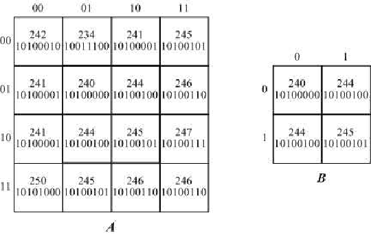
Initially,

\begin{split}\Psi_{0}&=|g\rangle\otimes|f\rangle\otimes|A\rangle\otimes|B\rangle\\ &=|g\rangle\otimes\left(\frac{1}{8}|0\rangle|10100010\rangle|0000\rangle|10100000\rangle|00\rangle+\frac{1}{8}|0\rangle|10100010\rangle|0000\rangle|10100100\rangle|01\rangle\right.\\ &+\frac{1}{8}|0\rangle|10100010\rangle|0000\rangle|10100100\rangle|10\rangle+\frac{1}{8}|0\rangle|10100010\rangle|0000\rangle|10100101\rangle|11\rangle+\frac{1}{8}|0\rangle|10011100\rangle|0001\rangle|10100000\rangle|00\rangle\\ &+\frac{1}{8}|0\rangle|10011100\rangle|0001\rangle|10100100\rangle|01\rangle+\frac{1}{8}|0\rangle|10011100\rangle|0001\rangle|10100100\rangle|10\rangle+\frac{1}{8}|0\rangle|10011100\rangle|0001\rangle|10100101\rangle|11\rangle\\ &+\frac{1}{8}|0\rangle|10100001\rangle|0010\rangle|10100000\rangle|00\rangle+\frac{1}{8}|0\rangle|10100001\rangle|0010\rangle|10100100\rangle|01\rangle+\frac{1}{8}|0\rangle|10100001\rangle|0010\rangle|10100100\rangle|10\rangle\\ &+\frac{1}{8}|0\rangle|10100001\rangle|0010\rangle|10100101\rangle|11\rangle+\frac{1}{8}|0\rangle|10100101\rangle|0011\rangle|10100000\rangle|00\rangle+\frac{1}{8}|0\rangle|10100101\rangle|0011\rangle|10100100\rangle|01\rangle\\ &+\frac{1}{8}|0\rangle|10100101\rangle|0011\rangle|10100100\rangle|10\rangle+\frac{1}{8}|0\rangle|10100101\rangle|0011\rangle|10100101\rangle|11\rangle+\frac{1}{8}|0\rangle|10100001\rangle|0100\rangle|10100000\rangle|00\rangle\\ &+\frac{1}{8}|0\rangle|10100001\rangle|0100\rangle|10100100\rangle|01\rangle+\frac{1}{8}|0\rangle|10100001\rangle|0100\rangle|10100100\rangle|10\rangle+\frac{1}{8}|0\rangle|10100001\rangle|0100\rangle|10100101\rangle|11\rangle\\ &+\frac{1}{8}|0\rangle|10100000\rangle|0101\rangle|10100000\rangle|00\rangle+\frac{1}{8}|0\rangle|10100000\rangle|0101\rangle|10100100\rangle|01\rangle+\frac{1}{8}|0\rangle|10100000\rangle|0101\rangle|10100100\rangle|10\rangle\\ &+\frac{1}{8}|0\rangle|10100000\rangle|0101\rangle|10100101\rangle|11\rangle+\frac{1}{8}|0\rangle|10100100\rangle|0110\rangle|10100000\rangle|00\rangle+\frac{1}{8}|0\rangle|10100100\rangle|0110\rangle|10100100\rangle|01\rangle\\ &+\frac{1}{8}|0\rangle|10100100\rangle|0110\rangle|10100100\rangle|10\rangle+\frac{1}{8}|0\rangle|10100100\rangle|0110\rangle|10100101\rangle|11\rangle+\frac{1}{8}|0\rangle|10100110\rangle|0111\rangle|10100000\rangle|00\rangle\\ &+\frac{1}{8}|0\rangle|10100110\rangle|0111\rangle|10100100\rangle|01\rangle+\frac{1}{8}|0\rangle|10100110\rangle|0111\rangle|10100100\rangle|10\rangle+\frac{1}{8}|0\rangle|10100110\rangle|0111\rangle|10100101\rangle|11\rangle\\ &+\frac{1}{8}|0\rangle|10100001\rangle|1000\rangle|10100000\rangle|00\rangle+\frac{1}{8}|0\rangle|10100001\rangle|1000\rangle|10100100\rangle|01\rangle+\frac{1}{8}|0\rangle|10100001\rangle|1000\rangle|10100100\rangle|10\rangle\\ &+\frac{1}{8}|0\rangle|10100001\rangle|1000\rangle|10100101\rangle|11\rangle+\frac{1}{8}|0\rangle|10100100\rangle|1001\rangle|10100000\rangle|00\rangle+\frac{1}{8}|0\rangle|10100100\rangle|1001\rangle|10100100\rangle|01\rangle\\ &+\frac{1}{8}|0\rangle|10100100\rangle|1001\rangle|10100100\rangle|10\rangle+\frac{1}{8}|0\rangle|10100100\rangle|1001\rangle|10100101\rangle|11\rangle+\frac{1}{8}|0\rangle|10100101\rangle|1010\rangle|10100000\rangle|00\rangle\\ &+\frac{1}{8}|0\rangle|10100101\rangle|1010\rangle|10100100\rangle|01\rangle+\frac{1}{8}|0\rangle|10100101\rangle|1010\rangle|10100100\rangle|10\rangle+\frac{1}{8}|0\rangle|10100101\rangle|1010\rangle|10100101\rangle|11\rangle\\ &+\frac{1}{8}|0\rangle|10100111\rangle|1011\rangle|10100000\rangle|00\rangle+\frac{1}{8}|0\rangle|10100111\rangle|1011\rangle|10100100\rangle|01\rangle+\frac{1}{8}|0\rangle|10100111\rangle|1011\rangle|10100100\rangle|10\rangle\\ &+\frac{1}{8}|0\rangle|10100111\rangle|1011\rangle|10100101\rangle|11\rangle+\frac{1}{8}|0\rangle|10101000\rangle|1100\rangle|10100000\rangle|00\rangle+\frac{1}{8}|0\rangle|10101000\rangle|1100\rangle|10100100\rangle|01\rangle\\ &+\frac{1}{8}|0\rangle|10101000\rangle|1100\rangle|10100100\rangle|10\rangle+\frac{1}{8}|0\rangle|10101000\rangle|1100\rangle|10100101\rangle|11\rangle+\frac{1}{8}|0\rangle|10100101\rangle|1101\rangle|10100000\rangle|00\rangle\\ &+\frac{1}{8}|0\rangle|10100101\rangle|1101\rangle|10100100\rangle|01\rangle+\frac{1}{8}|0\rangle|10100101\rangle|1101\rangle|10100100\rangle|10\rangle+\frac{1}{8}|0\rangle|10100101\rangle|1101\rangle|10100101\rangle|11\rangle\\ &+\frac{1}{8}|0\rangle|10100110\rangle|1110\rangle|10100000\rangle|00\rangle+\frac{1}{8}|0\rangle|10100110\rangle|1110\rangle|10100100\rangle|01\rangle+\frac{1}{8}|0\rangle|10100110\rangle|1110\rangle|10100100\rangle|10\rangle\\ &+\frac{1}{8}|0\rangle|10100110\rangle|1110\rangle|10100101\rangle|11\rangle+\frac{1}{8}|0\rangle|10100110\rangle|1111\rangle|10100000\rangle|00\rangle+\frac{1}{8}|0\rangle|10100110\rangle|1111\rangle|10100100\rangle|01\rangle\\ &\left.+\frac{1}{8}|0\rangle|10100110\rangle|1111\rangle|10100100\rangle|10\rangle+\frac{1}{8}|0\rangle|10100110\rangle|1111\rangle|10100101\rangle|11\rangle\right)\end{split}

Step 1 changes $I_{A}^{i}$ to $I_{A}^{i}\oplus I_{B}^{i}$ and Step 2 changes $|f\rangle$ to $|1\rangle$ when $|I_{A}\rangle=|0\rangle^{\otimes q}$ and $|k_{B}\rangle=|0\rangle^{\otimes m}$ . Hence,

\begin{split}\Psi_{2}&=|g\rangle\otimes|f\rangle\otimes|A\rangle\otimes|B\rangle\\ &=|g\rangle\otimes\left(\frac{1}{8}|0\rangle|00000010\rangle|0000\rangle|10100000\rangle|00\rangle+\frac{1}{8}|0\rangle|00000110\rangle|0000\rangle|10100100\rangle|01\rangle\right.\\ &+\frac{1}{8}|0\rangle|00000110\rangle|0000\rangle|10100100\rangle|10\rangle+\frac{1}{8}|0\rangle|00000111\rangle|0000\rangle|10100101\rangle|11\rangle+\frac{1}{8}|0\rangle|00111100\rangle|0001\rangle|10100000\rangle|00\rangle\\ &+\frac{1}{8}|0\rangle|00111000\rangle|0001\rangle|10100100\rangle|01\rangle+\frac{1}{8}|0\rangle|00111000\rangle|0001\rangle|10100100\rangle|10\rangle+\frac{1}{8}|0\rangle|00111001\rangle|0001\rangle|10100101\rangle|11\rangle\\ &+\frac{1}{8}|0\rangle|00000001\rangle|0010\rangle|10100000\rangle|00\rangle+\frac{1}{8}|0\rangle|00000101\rangle|0010\rangle|10100100\rangle|01\rangle+\frac{1}{8}|0\rangle|00000101\rangle|0010\rangle|10100100\rangle|10\rangle\\ &+\frac{1}{8}|0\rangle|00000100\rangle|0010\rangle|10100101\rangle|11\rangle+\frac{1}{8}|0\rangle|00000101\rangle|0011\rangle|10100000\rangle|00\rangle+\frac{1}{8}|0\rangle|00000001\rangle|0011\rangle|10100100\rangle|01\rangle\\ &+\frac{1}{8}|0\rangle|00000001\rangle|0011\rangle|10100100\rangle|10\rangle+\frac{1}{8}|0\rangle|00000000\rangle|0011\rangle|10100101\rangle|11\rangle+\frac{1}{8}|0\rangle|00000001\rangle|0100\rangle|10100000\rangle|00\rangle\\ &+\frac{1}{8}|0\rangle|00000101\rangle|0100\rangle|10100100\rangle|01\rangle+\frac{1}{8}|0\rangle|00000101\rangle|0100\rangle|10100100\rangle|10\rangle+\frac{1}{8}|0\rangle|00000100\rangle|0100\rangle|10100101\rangle|11\rangle\\ &+\boxed{\frac{1}{8}|1\rangle|00000000\rangle|0101\rangle|10100000\rangle|00\rangle}+\frac{1}{8}|0\rangle|00000100\rangle|0101\rangle|10100100\rangle|01\rangle+\frac{1}{8}|0\rangle|00000100\rangle|0101\rangle|10100100\rangle|10\rangle\\ &+\frac{1}{8}|0\rangle|00000101\rangle|0101\rangle|10100101\rangle|11\rangle+\frac{1}{8}|0\rangle|00000100\rangle|0110\rangle|10100000\rangle|00\rangle+\frac{1}{8}|0\rangle|00000000\rangle|0110\rangle|10100100\rangle|01\rangle\\ &+\frac{1}{8}|0\rangle|00000000\rangle|0110\rangle|10100100\rangle|10\rangle+\frac{1}{8}|0\rangle|00000001\rangle|0110\rangle|10100101\rangle|11\rangle+\frac{1}{8}|0\rangle|00000110\rangle|0111\rangle|10100000\rangle|00\rangle\\ &+\frac{1}{8}|0\rangle|00000010\rangle|0111\rangle|10100100\rangle|01\rangle+\frac{1}{8}|0\rangle|00000010\rangle|0111\rangle|10100100\rangle|10\rangle+\frac{1}{8}|0\rangle|00000011\rangle|0111\rangle|10100101\rangle|11\rangle\\ &+\frac{1}{8}|0\rangle|00000001\rangle|1000\rangle|10100000\rangle|00\rangle+\frac{1}{8}|0\rangle|00000101\rangle|1000\rangle|10100100\rangle|01\rangle+\frac{1}{8}|0\rangle|00000101\rangle|1000\rangle|10100100\rangle|10\rangle\\ &+\frac{1}{8}|0\rangle|00000100\rangle|1000\rangle|10100101\rangle|11\rangle+\frac{1}{8}|0\rangle|00000100\rangle|1001\rangle|10100000\rangle|00\rangle+\frac{1}{8}|0\rangle|00000000\rangle|1001\rangle|10100100\rangle|01\rangle\\ &+\frac{1}{8}|0\rangle|00000000\rangle|1001\rangle|10100100\rangle|10\rangle+\frac{1}{8}|0\rangle|00000001\rangle|1001\rangle|10100101\rangle|11\rangle+\frac{1}{8}|0\rangle|00000101\rangle|1010\rangle|10100000\rangle|00\rangle\\ &+\frac{1}{8}|0\rangle|00000001\rangle|1010\rangle|10100100\rangle|01\rangle+\frac{1}{8}|0\rangle|00000001\rangle|1010\rangle|10100100\rangle|10\rangle+\frac{1}{8}|0\rangle|00000000\rangle|1010\rangle|10100101\rangle|11\rangle\\ &+\frac{1}{8}|0\rangle|00000111\rangle|1011\rangle|10100000\rangle|00\rangle+\frac{1}{8}|0\rangle|00000011\rangle|1011\rangle|10100100\rangle|01\rangle+\frac{1}{8}|0\rangle|00000011\rangle|1011\rangle|10100100\rangle|10\rangle\\ &+\frac{1}{8}|0\rangle|00000010\rangle|1011\rangle|10100101\rangle|11\rangle+\frac{1}{8}|0\rangle|00001000\rangle|1100\rangle|10100000\rangle|00\rangle+\frac{1}{8}|0\rangle|00001100\rangle|1100\rangle|10100100\rangle|01\rangle\\ &+\frac{1}{8}|0\rangle|00001100\rangle|1100\rangle|10100100\rangle|10\rangle+\frac{1}{8}|0\rangle|00001101\rangle|1100\rangle|10100101\rangle|11\rangle+\frac{1}{8}|0\rangle|00000101\rangle|1101\rangle|10100000\rangle|00\rangle\\ &+\frac{1}{8}|0\rangle|00000001\rangle|1101\rangle|10100100\rangle|01\rangle+\frac{1}{8}|0\rangle|00000001\rangle|1101\rangle|10100100\rangle|10\rangle+\frac{1}{8}|0\rangle|00000000\rangle|1101\rangle|10100101\rangle|11\rangle\\ &+\frac{1}{8}|0\rangle|00000110\rangle|1110\rangle|10100000\rangle|00\rangle+\frac{1}{8}|0\rangle|00000010\rangle|1110\rangle|10100100\rangle|01\rangle+\frac{1}{8}|0\rangle|00000010\rangle|1110\rangle|10100100\rangle|10\rangle\\ &+\frac{1}{8}|0\rangle|00000011\rangle|1110\rangle|10100101\rangle|11\rangle+\frac{1}{8}|0\rangle|00000110\rangle|1111\rangle|10100000\rangle|00\rangle+\frac{1}{8}|0\rangle|00000010\rangle|1111\rangle|10100100\rangle|01\rangle\\ &\left.+\frac{1}{8}|0\rangle|00000010\rangle|1111\rangle|10100100\rangle|10\rangle+\frac{1}{8}|0\rangle|00000011\rangle|1111\rangle|10100101\rangle|11\rangle\right)\end{split}

The boxed pixel is the one that we want to find out.

Hence, in the subspace $|k_{A}\rangle$ .

\Psi_{30}=\left(\frac{1}{4},\frac{1}{4},\frac{1}{4},\frac{1}{4},\frac{1}{4},\boxed{\frac{1}{4}},\frac{1}{4},\frac{1}{4},\frac{1}{4},\frac{1}{4},\frac{1}{4},\frac{1}{4},\frac{1}{4},\frac{1}{4},\frac{1}{4},\frac{1}{4}\right)^{\text{T}}

It should be iterated

\hat{i}=\left\lceil-1+\frac{1}{2}\sqrt{4-\frac{2}{3}c+A+B}-\frac{1}{2}\sqrt{8-\frac{4}{3}c-A-B}\right\rceil=3

times.

\bullet

for the first iteration:

\begin{split}&\overline{t}_{1}=\left.\left(15\cdot\frac{1}{4}-\frac{1}{4}\right)\middle/16\right.=\frac{7}{32}\\ &t_{10}=2\cdot\frac{7}{32}+\frac{1}{4}=\frac{11}{16},\ \ \ t_{1}=2\cdot\frac{7}{32}-\frac{1}{4}=\frac{3}{16}\end{split}

\bullet

for the second iteration:

\begin{split}&\overline{t}_{2}=\left.\left(15\cdot\frac{3}{16}-\frac{11}{16}\right)\middle/16\right.=\frac{17}{128}\\ &t_{20}=2\cdot\frac{17}{128}+\frac{11}{16}=\frac{61}{64},\ \ \ t_{2}=2\cdot\frac{17}{128}-\frac{3}{16}=\frac{5}{64}\end{split}

\bullet

for the third iteration:

\begin{split}&\overline{t}_{3}=\left.\left(15\cdot\frac{5}{64}-\frac{61}{64}\right)\middle/16\right.=\frac{7}{512}\\ &t_{30}=2\cdot\frac{7}{512}+\frac{61}{64}=\frac{251}{256},\ \ \ t_{3}=2\cdot\frac{7}{512}-\frac{5}{64}=-\frac{13}{256}\end{split}

After 3 times of iterations, the sixth basis $|0101\rangle$ will be measured with probability $\left(\frac{251}{256}\right)^{2}=0.9613$ which is much higher than the probability $\left(-\frac{13}{256}\right)^{2}=0.002579$ of other pixels being measured.

In this example, if it is iterated 4 times, $t_{40}$ will be $\frac{781}{1024}<\frac{251}{256}$ . Hence, Theorem 1 and 2 are verified.

Moreover, $t_{30}^{2}=0.9613>(0.9194+0.0567a^{-1}+0.2302a^{-2}-0.0336a^{-3})^{2}=0.8976$ . Hence, Theorem 3 is verified.

5 Complexity analysis

In this scheme, the main step is Step 3 which has $\hat{i}$ iterations. According to Theorem 1 or 2, $\hat{i}$ is a $O(a)$ , i.e., $O(2^{n})$ order polynomial. Hence the network complexity of quantum image matching is $O(2^{n})$ .

Compared with the complexity of the classical image matching: $O(2^{2n+2m})$ , the quantum algorithm dropped the complexity obviously.

6 Discussions and conclusions

In this paper, we try to solve the problem of measurement and give a quantum image matching algorithm.

The contributions of this paper include:

1.

Give a quantum image matching scheme which can find out a small image in a big image. The entanglement property of quantum sates make all the pixels be processed simultaneously, which improves the scheme’s effectiveness.
2.

Solve the problem of measurement based on Grover’s algorithm. Our scheme can get the right answer with high probability by being processed and measured only once, which helps to truly drop the scheme’s complexity. This is the main advantage compared with the most existing quantum image processing algorithms.

Future works, or something that should be discussed include:

The number of the matching areas.

If the small image is only matched with one area in the big image (like we discussed above), our solution is a good choice. However, if there are no or more than one matching areas, some problems will arise:

\bullet

More than one areas.

If there are $l$ ( $l>1$ ) matched areas, Eq. (16) will have more than one $-\frac{1}{2}$ . As a consequence, the state before measurement will be

\Psi_{33}=\left(t_{\hat{i}},\cdots,t_{\hat{i}},t_{\hat{i}0},t_{\hat{i}},\cdots,t_{\hat{i}},t_{\hat{i}0},t_{\hat{i}},\cdots,t_{\hat{i}}\right)^{\text{T}},

Hence, one of and only one of the $l$ matched areas will be measured randomly.

$\bullet$

No area.

If there are no matched areas, in Eq. (16), all the elements of $\Psi_{31}$ are $\frac{1}{2}$ . According to Eq. (28), no matter how many times Step 3 is iterated, the output state of Step 3 will be

$\Psi_{33}=\left(\frac{1}{2^{n}},\cdots,\frac{1}{2^{n}},\frac{1}{2^{n}},\frac{1}{2^{n}},\cdots,\frac{1}{2^{n}}\right)^{\text{T}}.$

Hence, an arbitrary pixel will be measured randomly.

The above two points indicate that our scheme is not good at the multi-matching-area or none-matching-area problem. This is one of the future work.

2.

Fuzzy matching.

Our scheme can only solve the problem of precisely matching. If the images have some deformations such as shown in Fig. 4, the scheme will fail. Hence, we plan to solve the matching problem with deformations in the future papers.

Acknowledgements.

The authors thank Prof. Sabre Kais and Phd. Student Yudong Cao at Purdue University for their valuable suggestions.

References

(1) Feynman R.P. Simulating physics with computers. Int. J. Theor. Phys. 21(6/7): 467-488 (1982)
(2) Vasil S. Denchev, Sergio Boixo, Sergei V. Isakov, and etc. What is the computational value of finite range tunneling? arXiv:1512.02206v4 (2016)
(3) Le, P.Q., Iliyasu, A.M., Dong, F.Y., Hirota, K.: Fast geometric transformation on quantum images. IAENG Int. J. Appl. Math. 40(3), 113-123 (2010)
(4) Wang, J., Jiang, N., Wang, L.: Quantum image translation. Quantum Inf. Process, 14(5), 1589-1604 (2015)
(5) Jiang, N., Wang, L.: Quantum image scaling using nearest neighbor interpolation. Quantum Inf. Process, 14(5), 1559-1571 (2015)
(6) Jiang, N., Wang, J., Mu, Y.: Quantum image scaling up based on nearest-neighbor interpolation with integer scaling ratio. Quantum Inf. Process, 14(11), 4001-4026 (2015)
(7) Zhang, Y., Lu, K., Gao, Y.H., Wang, M.: NEQR: a novel enhanced quantum representation of digital images. Quantum Inf. Process, 12(12), 2833-2860 (2013)
(8) Jiang, N., Wu, W.Y., Wang, L., Zhao, N.: Quantum image pseudocolor coding based on the density-stratified method. Quantum Inf. Process, 14(5), 1735-1755 (2015)
(9) Jiang, N., Wu, W.Y., Wang, L.: The quantum realization of Arnold and Fibonacci image scrambling. Quantum Inf. Process, 13(5), 1223-1236 (2014)
(10) Jiang, N., Wang, L.: Analysis and improvement of the quantum Arnold image scrambling. Quantum Inf. Process, 13(7), 1545-1551 (2014)
(11) Jiang, N., Wang, L., Wu, W.Y.: Quantum Hilbert image scrambling. International Journal of Theoretical Physics, 53(7), 2463-2484 (2014)
(12) Venegas-Andraca S.E., Ball J.L.: Processing images in entangled quantum systems. Quantum Information Processing 9(1), 1-11 (2010)
(13) Li, H.S., Zhu, Q.X., Lan, S., Shen, C.Y., Zhou, R.G., Mo, J.: Image storage, retrieval, compression and segmentation in a quantum system. Quantum Inf. Process, 12(6), 2269-2290 (2013)
(14) Caraiman, S., Manta, V.: Histogram-based segmentation of quantum images. Theor. Comput. Sci. 529, 46-60 (2014)
(15) Zhang, Y., Lu, K., Xu, K., Gao, Y.H., Wilson, R.: Local feature point extraction for quantum images. Quantum Inf. Process, published online (2014)
(16) Iliyasu, A.M., Le, P.Q., Dong, F., Hirota, K.: Watermarking and authenticationof quantum images based on restricted geometric transformations. Information Sciences, 186, 126-149 (2012)
(17) Zhang, W.W., Gao, F., Liu, B., etc.: A watermark strategy for quantum images based on quantum Fourier transform. Quantum Information Processing, 12(4), 793-803 (2013)
(18) Zhang, W.W., Gao, F., Liu, B., etc.: A quantum watermark protocol. International Journal of Theory Physics, 52: 504-513 (2013)
(19) Yang Y.G., Jia X., Xu P.,Tian J. Analysis and improvement of the watermark strategy for quantum images based on quantum Fourier transform. Quantum Information Processing, 2013, 12(8): 2765-2769.
(20) Song X.H., Wang S., Liu S., Ahmed A. Abd El-Latif, Niu X.M.: A dynamic watermarking scheme for quantum images using quantum wavelet transform. Quantum Information Processing, 12(12), 3689-3706 (2013)
(21) Song X.H., Wang S., Liu S., Ahmed A. Abd El-Latif, Niu X.M.: Dynamic watermarking scheme for quantum images based on Hadamard transform. Multimedia Systems, published online (2014)
(22) Jiang N., Wang L.: A quantum image information hiding algorithm based on Moir $\acute{e}$ pattern. International Journal of Theoretical Physics, published online (2014)
(23) Jiang, N., Zhao, N., Wang, L.: LSB based quantum image steganography algorithm. International Journal of Theoretical Physics, 55(1), 107-123 (2016)
(24) Wang S., Song X.H., Niu X.M.: A Novel Encryption Algorithm for Quantum Images Based on Quantum Wavelet Transform and Diffusion. Intelligent Data analysis and its Applications, Volume II, 298, 243-250 (2014)
(25) Hua Tianxiang, Chen Jiamin, Pei Dongju and etc. Quantum Image Encryption Algorithm Based on Image Correlation Decomposition. International Journal of Theoretical Physics, published online (2014)
(26) Zhou Ri-Gui, Wu Qian, Zhang Man-Qun and etc. A Quantum Image Encryption Algorithm Based on Quantum Image Geometric Transformations. Pattern Recognition, 2012, 321: 480-487.
(27) Zhou Ri-Gui, Wu Qian, Zhang Man-Qun and etc. Quantum Image Encryption and Decryption Algorithms Based on Quantum Image Geometric Transformations. International Journal of Theoretical Physics, 2013, 52:1802-1817.
(28) Barbara Zitov $\acute{a}$ , Jan Flusser: Image registration methods: a survey. Image Vision Comput. 21(11), 977-1000 (2003)
(29) https://en.wikipedia.org/wiki/Image registration
(30) http://web.eecs.umich.edu/ silvio/teaching/EECS598 2010/slides/09 30 Alok Sairam.pdf
(31) Lov K. Grover. A fast quantum mechanical algorithm for database search. In: Proceedings of the 28th Annual ACM Symposium on the Theory of Computing: 212-219 (1996)
(32) Marco Genovese. Real applications of quantum imaging. arXiv:1601.06066v1: 1-18 (2016)
(33) Sun, J.G., He, Y.G.: A quantum search algorithm. Journal of Software. 14(3): 334-344 (2003)
(34) Yang, Y.G., Zhao, Q.Q., Sun, S.J. Novel quantum gray-scale image matching. Optik. 126: 3340-3343 (2015)
(35) Liu, F., Duan, H.B., Deng, Y.M. A chaotic quantum-behaved particle swarm optimization based on lateral inhibition for image matching. Optik. 123: 1955-1960 (2012)
(36) Khalil M. Mezghiche, Kamal E. Melkemi, Sebti Foufou. Matching with quantum genetic algorithm and shape contexts. 2014 IEEE/ACS 11th International Conference on Computer Systems and Applications (AICCSA): 536-542 (2014)
(37) Daniel Curtis, David A. Meyer. Towards quantum template matching. Proc. SPIE 5161, Quantum Communications and Quantum Imaging: 134-141 (2004)
(38) Mastriani, M.: Quantum image processing? arXiv:1512.02942. 1-28 (2015)
(39) Mastriani, M.: Quantum Boolean image denoising. Springer Quantum Information Processing. 14(5), 1647-1673 (2015)