Isospin Invariance and the Vacuum Polarization Energy of Cosmic Strings
Abstract
We corroborate the previously applied spectral approach to compute the vacuum polarization energy of string configurations in models similar to the standard model of particle physics. The central observation underlying this corroboration is the existence of a particular global isospin transformation of the string configuration. Under this transformation the single particle energies of the quantum fluctuations are invariant, while the inevitable implementation of regularization and renormalization requires operations that are not invariant. We verify numerically that all such variances eventually cancel, and that the vacuum polarization energy obtained in the spectral approach is indeed gauge invariant.
I Introduction
Various field theories suggest the existence of stringlike configurations, which are the particle physics analogs of vortices or magnetic flux tubes in condensed matter physics. These configurations can arise at scales ranging from the fundamental distances in string theory to astrophysical distances, where in the latter case they are often called cosmic strings. (See for example the reviews [1, 2].)11 1 Arguments for a closer connection between cosmic and fundamental strings are given in Ref. [3]. A well–known representative is the Nielsen–Olesen vortex [4] in a model with an Abelian gauge field coupled to a single Higgs field. This vortex is classically stable, as are particular embeddings in non–Abelian models with several Higgs fields [5]. In general, however, non–Abelian string configurations are not classically stable. In this context the –string, which typically involves the –boson field in the standard model, is of particular interest [6]. Though not classically stable, it is possible that these strings are stabilized by quantum effects. The vacuum polarization energy (VPE), which is the regularized and renormalized sum of all zero point energies of the quantum fluctuations in the classical background, is central to these investigations. In field theory quantum effects are typically estimated by Feynman diagram techniques. However, stringlike configurations have a nontrivial structure at spatial infinity which makes the formulation of a Feynman perturbation expansion impossible without any further adaptation. Even then, the convergence of the series is not guaranteed as the relevant couplings are not necessarily small and the series is only asymptotic. On top of that, the rich topological structures [7] of theories with cosmic strings require techniques beyond perturbative treatments. Not surprisingly, the study of the VPE of cosmic string configurations has a long history of slow progress without a fully concluding answer.
Numerous publications have analyzed quantum fluctuations about cosmic strings. Naculich [8] has discussed that in the limit of weak coupling, fermion fluctuations tend to destabilize the string. The quantum properties of –strings have also been connected to nonperturbative anomalies [9]. Furthermore, the emergence or absence of exact neutrino zero modes in a –string background and the possible consequences for the string topology were investigated in Ref. [10]. A first attempt at a full calculation of the fermion quantum corrections to the –string energy was carried out in Ref. [11]. Those authors were only able to compare the energies of two string configurations, rather than comparing a single string to the vacuum, because of limitations arising from the nontrivial behavior at spatial infinity. (We will discuss this issue in more detail below.) The fermion vacuum polarization energy of the Abelian Nielsen–Olesen vortex [4] has been estimated in Ref. [12] with regularization limited to the subtraction of the divergences in the heat–kernel expansion. On the other hand, quantum energies of bosonic fluctuations in string backgrounds were calculated in Ref. [13]. However, these are suppressed compared to fermion fluctuations when the number of internal degrees of freedom, e.g. color, is large.
Using the spectral method [14] the (one–loop) VPE can be computed from scattering data. An essential feature of this method is the identification of elements from the Born expansion with Feynman diagrams. These elements are added and subtracted to make contact with standard renormalization techniques and conditions which prescribe certain Green functions for particular values of transferred momenta. In a sequence of projects we succeeded computing the fermion VPE of cosmic strings after solving a number of problems:22 2 See Ref. [15] for a recent review.
- 1.
The string configuration does not have a well defined Born series to be identified with the Feynman series of quantum field theory; this can be overcome by a special local gauge transformation [16].
- 2.
- 3.
Higher order Feynman diagrams are required which become exceedingly difficult to evaluate numerically; this is solved by the so-called fake boson approach [19].
Formally the unregularized and unrenormalized fermion VPE of the string is the sum of energy eigenvalues from a Dirac Hamiltonian. These eigenvalues are invariant for a particular path in the space of parameters which define the (weak) isospin orientation of the string [20]. Previous calculations of the VPE [16, 17, 18] were restricted to a simplifying submanifold in isospace that could not access this path. The invariance of the single particle energies is, however, not sufficient to ensure that the full fermion VPE is also invariant in this calculation. The sum of the energy eigenvalues is ultraviolet divergent and in the inevitable process of regularization and renormalization divergent contributions emerge that are manifestly variant. They are conjectured to cancel based on their formal equivalence as expansions in powers of the string background. On the regularization side terms from the Born expansion to scattering data are subtracted, which on the renormalization side are added back in the form of Feynman diagrams. An exact match of these quantities is not at all obvious. For instance, Feynman diagrams allow us to distinguish between the divergences that emerge from the quantum loops and the Fourier modes of the background (this is e.g. essential for understanding the Casimir effect [21] in the context of spectral methods). On the other hand scattering data, and thus the Born expansion terms, do not distinguish between external and loop momenta. Using dimensional regularization, the equivalence of the two schemes has been verified for the leading (tadpole) divergence, both for boson [22] and fermion[23] fluctuations. At higher order the distinction between loop and Fourier momenta is essential and so far no such proof has been provided.
The scattering data decouple into angular momentum channels. As we will explain in Sec. III, a channel by channel subtraction is mandatory for contributions that can be related to the quadratic ultraviolet divergences in the Feynman series. The subleading logarithmic divergences require to include higher order Born/Feynman terms, which are very cumbersome to simulate numerically. Fortunately, the set of divergences terminates at this logarithmic level so that these divergences can be cavalierly treated by simulating them in a simpler (typically bosonic) theory. This method brings into the game an additional contribution that is not manifestly invariant under the particular isospin transformation mentioned above. Furthermore, the simulation of divergences by a boson model also requires the exchange of momentum integrals with orbital angular momentum sums. which by itself demands care: for instance, swapping these operations for momenta on the real axis gives erroneous results [24]; instead, an analytic continuation to imaginary momenta is required [25]. In any event, the whole regularization procedure is not manifestly gauge invariant while gauge invariance should, of course, be maintained by the final result in order for the adopted calculational procedure to produce unambiguous results. A good example to demonstrate the subtleties of gauge invariance in the context of the spectral approach are the vacuum charges induced by a nontrivial background configuration: improper regularization may falsely predict anomalous vacuum charges [23]. From these considerations, it is clear that consistency checks are indispensable to ensure that the spectral method does not artificially break (gauge) symmetries leading to erroneous results. In the present paper, we will explore such a test based on a global isospin invariance. Because of the operation under item 1) above, this also probes a local invariance.
We conclude this introduction with a brief description of our model. The bosonic part is described by the Lagrangian
| (1) |
where the Higgs doublet is written using the matrix representation
| (2) |
The gauge coupling constant enters through both the covariant derivative and the field strength tensor
| (3) |
The classical potential has been chosen such that the Higgs field acquires a vacuum expectation value (VEV) , where . As a consequence, all bosons become massive: and . The interaction of the (classical) string with the left–handed fermions is described by
| (4) |
Here, are projection operators on left/right–handed components, respectively, and the strength of the Higgs-fermion interaction is parametrized by the Yukawa coupling , which gives rise to the fermion mass, .
This short report is organized as follows. In Sec. II we discuss the particular form of the cosmic string configuration and describe the path in weak isospace along which the Dirac eigenvalues are unchanged. In section III we explain how spectral methods are utilized to compute the fermion contribution to the VPE, including the subtleties needed to make the approach feasible. We present numerical results for the VPE in section IV and show that this particular invariance is indeed reproduced within our numerical accuracy. We conclude with a brief summary in Sec. V and leave some technical details to appendixes.
II Cosmic String Configuration
The starting point to parametrize cosmic string configurations is the four dimensional unit vector [26, 27]
| (5) |
where and describe the isospin orientation of the string and is the azimuthal angle in coordinate space.33 3 The string configuration will be infinitely extended along the -direction in coordinate space. For simplicity, we will always consider unit winding of the string; generalizations to winding number merely require the replacement and . In what follows we also employ the abbreviations
| (6) |
for the trigonometrical functions of the isospin angles and . A global rotation within the plane of the second and third components by an angle with transforms the unit vector into
| (7) |
Hence observables (which are, by definition, gauge invariant) will not depend on the two angles and individually but only on the product . Stated otherwise, all observables must remain invariant along paths of constant in isospin space [20].
The unit vector defines the matrix , where are the three Pauli matrices. The Higgs and gauge fields of the string are then characterized by two profile functions and that are functions of the distance () from the string center:
| (8) |
Here, the gauge connection is a vector in coordinate space and a matrix in the adjoint representation of weak isospace. The profile functions vanish at the core of the string () and approach unity at spatial infinity. From this parametrization we find the classical mass of the string44 4 Here and in the following, the prime indicates a derivative with respect to the radial argument , and we omit the argument for simplicity if no confusion can occur.
| (9) |
where the dimensionless radial integration variable is related to the physical radius by and we have introduced the mass ratio . As expected, the classical mass only depends on the isospin angles via the combination , which reflects gauge invariance.
Note that the configuration, Eq. (8) approaches a local gauge transformation of the constant vacuum configuration at spatial infinity. As a consequence, this configuration is not appropriate for techniques that require some kind of perturbative expansions which do not preserve gauge invariance order by order. In particular, individual Fourier transformations of the Higgs and gauge fields are ill defined. We therefore introduce an additional radial function with the boundary values and to define the local gauge transformation
| (10) |
Since this gauge transformation does not introduce any singularity at the origin; at spatial infinity it accounts for the above mentioned gauge transformation of the constant vacuum. With the gauge transformation, Eq. (10) applied, perturbative expansions can be performed. Of course, this comes at the expense of an additional radial function. By construction, observables are independent of its detailed form as long as the boundary conditions described above are maintained. For the particular case of this was verified in Ref.[16]. In the present study, we will also consider deviations from that particular parameter value. We emphasize that the introduction of the gauge rotation, Eq. (10) has effectively made our test isospin symmetry local, since has turned into a space dependent quantity.
To write down the Dirac Hamiltonian from which we compute the spectrum of the fermion fluctuations we extract the Hamiltonian, from the Lagrangian, Eq. (4) and then perform the left–handed gauge transformation defined in Eq. (10): . To simplify the presentation we define and separate the interaction part (again using dimensionless variables)
| (11) | |||||
| (12) | |||||
The isopsin matrices in this expression are
| (13) |
Note that the latter appears with different arguments in Eq. (12). Nothing from the invariance along the path with is manifest in Eq. (12), neither is the gauge invariance from Eq. (10).
To proceed, we diagonalize the Hamiltonian in a basis of wave functions
| (14) |
that decouple radial and angular coordinates in the upper and lower components of the Dirac spinors ( refers to the energy eigenvalue defined in Eq. (17) below)
| (15) |
The notation is such that the signs denote the spin and isospin projection quantum numbers. For instance,
| (16) |
Diagonalization means that we construct the eigenvalues of the stationary Dirac equation
| (17) |
with . For we construct the full scattering matrix as a function of momentum . Since we employ four component Dirac spinors, we have and the spectrum is charge conjugation invariant. Our final result of the scattering problem (described in appendix A) is the Jost function for imaginary momentum , as well as the first two terms of its Born expansion obtained by iterating the interaction part .
III Vacuum Polarization Energy (VPE)
The main goal of the present investigation is to verify that our treatment of the ultraviolet divergences does not produce any dependence on the isospin angles and that cannot be expressed as . Any change in the renormalization conditions is described by finite counterterms. As was the case for the classical energy Eq. (9), the counterterms are manifestly functions of . We are therefore free to employ the simplest renormalization scheme, which is . For the profile functions we choose a specific form and introduce dimensionless width parameters , and :
| (18) |
Observable values for the width parameters are in units of since . Recall again that is just an auxiliary profile describing the local gauge transformation, Eq. (10), and that the VPE should be independent of . With these conventions on the ansatz parameters, the VPE depends on the model parameters , and only via the overall factor , see also Eq. (9). In this sense the dependence on the model parameters is completely contained in the classical energy and the counterterms, and thus requires little numerical effort.
The spectral method [14] to compute the VPE from scattering data identifies the change of the density of states caused by a static background as the derivative of the scattering phase shift (also known as the phase of the Jost function for real momenta) via the Krein–Friedel–Lloyd formula, cf. Ref. [28] and references therein. More precisely, we obtain the phase shift as , where is the scattering matrix of the multichannel problem. Integration over the momentum along the string then yields the VPE per unit length. However, that integral is only finite due to particular sum rules among the scattering data [29]. Ultimately this leads to the interface formalism [30] in which we only need to integrate over the momentum of the scattering problem in the plane perpendicular to the string. In this situation, it is prudent to use the analytic properties of the scattering data to perform the final momentum integral over imaginary momentum with . This analytic continuation has several advantages: First, it allows to interchange the momentum integral with the angular momentum sum [25] and second, it implicitly collects the contributions to the VPE coming from the bound states. This is beneficial, as there is generally a large number of such states, in particular for wide strings, and identifying them numerically is cumbersome. To express the VPE as an integral over imaginary momenta it is essential that the scattering phase shift is an odd function of the real momentum. Typically this property results from the Hamiltonian being real [32, 31] which is, however, not the case here: The gauge transformation, Eq. (10) turns the global isospin transformation along the path into a local one and, consequently, there is no global transformation on the basis states, Eq. (15) which could result in a real Hamiltonian.55 5 The Hamiltonian is still Hermitian, of course, and the single particle energies are real. In Appendix A we show that nevertheless the phase shift is odd in the momentum.
After collecting all information the VPE per unit length of the string is expressed as
| (19) |
where we performed a final change of variable to avoid the integrable singularity at . In Eq. (19) is the full Jost function with orbital angular momentum and degeneracy factor on the imaginary momentum axis, while and are first two terms of its Born expansion with respect to . These two subtractions are performed before summing over angular momentum channels. This is indispensable in order to identify and disentangle the subleading logarithmic divergence and the relevant finite contributions from the two leading Born terms. In fact, the logarithmic divergence has additional contributions from the third and fourth order Feynman diagrams, and their total strength66 6 Here, the term “strength” means that the Feynman diagrams produce the singularity in dimensional regularization. In Ref. [18] a factor 4 was omitted in the definition of both and , so that the ratio remains unaffected. is . The second order contribution of quantum corrections from a complex boson field about a static background also produces a logarithmic divergence. Let be its strength and the second order Born term of its Jost function for imaginary momenta in the angular momentum channel . Then the last term in curly brackets of Eq. (19) removes the logarithmic divergence from the integral. Since there is no further (sub–subleading) divergence, this subtraction can be made after summing over angular momenta. In the last step all subtractions are added back in the form of Feynman diagrams. They are computed by standard techniques using, e.g., dimensional regularization. Their divergent parts are uniquely compensated by counterterms in a definite renormalization scheme. All that remains are the finite parts and of the second order fermion and fake boson diagrams, which correspond to the finite parts of the subtractions and , respectively. Equation (19) is the master formula to compute the VEV of string configurations.
We stress that only the very first term under the integral in eq. (19) remains unchanged when varying the string isospin orientation, provided that remains constant. All other contributions are more general functions of and and thus vary along our particular isospin path of constant . These terms should eventually cancel provided that the identity of Born and Feynman series holds. However, individually they represent ill defined ultraviolet divergent quantities that undergo distinct regularization procedures and it is therefore unclear whether the spectral approach and, in particular, the renormalization procedure spoil gauge invariance. We will investigate this question numerically in the next section.
IV Results
The computation of the momentum integral and its integrand in Eq. (19) is by far the most expensive part of the numerical procedure. To begin with, the and channels require particular consideration. They involve Hankel functions of order zero whose irregular component diverges logarithmically at small arguments rather than by an inverse power law. Thus regular and irregular components are numerically difficult to separate. When integrating the radial differential equation [Eqs. (39) and (29) for ] we take the lower boundary to be for these two channels, and from we extrapolate to . In other channels a lower boundary of is fully reliable. Angular momenta are typically summed up to or above which numerical stability for Hankel functions at small arguments is lost. For background profiles with small or moderate widths this gives sufficient accuracy. Once the angular momentum sum is completed, the analog contribution from the fake boson (mimicking the logarithmic ultraviolet divergences from third and fourth order Feynman diagrams) is subtracted and the large behavior of the integrand is treated by fitting a tail, cf. the right panel of Fig. 1. Finally, for wider profiles an additional extrapolation of the angular momentum sum to is necessary which typically adds about to the VPE.
We start with a few examples, displayed in Table 1 and Fig. 1, in order to verify the independence from the gauge profile .
2.0 0.3010 -10.00 -0.0108 0.2902 0.3118 3.5 0.2974 -11.59 -0.0072 0.2902 0.3046 5.0 0.2953 -14.29 -0.0047 0.2905 0.3000 6.5 0.2915 -17.82 -0.0015 0.2901 0.2930
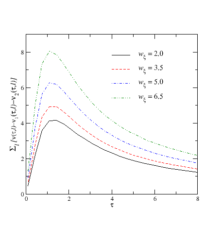
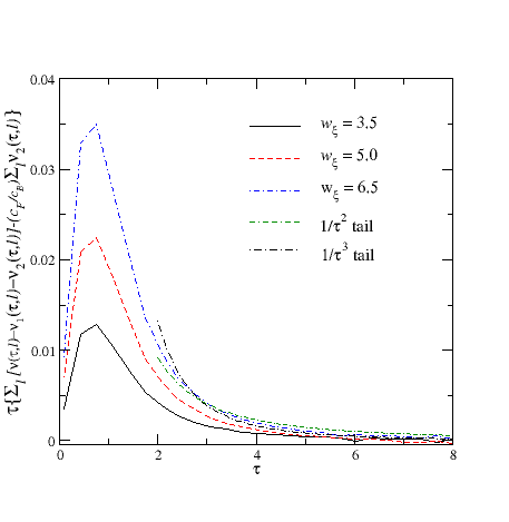
The variation of the individual contributions to the VPE is an order of magnitude larger than that of the total result. The tiny variation of the latter is due to errors from the numerical simulation. The cancellation of the gauge variant parts for the VPE is most obvious when adding them as absolute values which contains spreads of up to 10%. A large variation appears in the fermion part of the momentum integral (i.e. the contribution from the first term in curly brackets) in Eq. (19), as can be seen in Fig. 1.
Even though we have just established that the VPE does not vary with the width of the gauge profile, it is prudent for numerical efficiency and stability to choose that width similar to one in the profile functions of the physical boson fields, because otherwise large angular momenta play too significant a role.
0.1 0.4 0.1504 -4.913 0.0014 0.1518 0.1518 0.4 0.1 0.1702 -8.541 -0.0180 0.1521 0.1882 0.3 0.11834 0.1496 -6.814 0.0021 0.1517 0.1517 0.2 1/6 0.1639 -5.615 -0.0117 0.1522 0.1758

In Fig. 2 we show the strongly varying fermion part of the integrand for the VPE for sets of isospin angles that produce identical products . Despite the pronounced variation of this particular piece, the total VPE only differs at the order of the numerical accuracy as can clearly be seen from the data in Table 2. The comparison with the (incorrect) addition of the absolute values of the gauge variant contributions further illustrates this observation.
For the Hamiltonian is real. In this simpler case the VPE was computed for about 50 sets of width parameters (, , cf. Appendix B) and eight different values for in Ref. [18]. These results77 7 We have reproduced these earlier results for using the more general numerical simulation for the complex Hamiltonian. were then used to establish stable charged cosmic strings for fermion masses only slightly larger than that of the top quark. Here we consider the same sets of width parameters for two pairs of isospin angles that yield the identical products . In the first of the two pairs we simply swap the isospin angles as compared to the earlier calculations [18], and show the resulting VPE (in the renormalization scheme) in Fig. 3.


Obviously the computed VPEs agree within the numerical accuracy for the full range of considered width parameters. However, merely swapping the isospin angles is not sufficient to fully establish dependence on only the product . For example, there could be gauge variant contributions involving . To rule out such a dependence, we have made a second study and compared the two sets and . The resulting VPEs are shown in Fig. 4.


Again we observe perfect agreement for the computed VPEs as the tiny numerically discrepancies are not resolved within Figs. 3 and 4. So we conclude that the spectral methods to compute the VPE of cosmic strings indeed preserve gauge and isospin invariance even though some of its components do not.
The comparison of the results in Fig. 3 with those in Fig. 4 suggests that the VPE depends on the isospin orientation only mildly, except for the very narrow configurations that suffer from the Landau ghost problem [33, 34, 18]. This is not quite the case: in the current study our goal is to compare the VPE for configurations with equal , as in either of Figs. 3 or 4. To reveal the discussed invariance, the difference between the two angles is usually chosen deliberately large, so that one of the angles is always small and so is the product . When we lift this restriction we find e.g. with that increases from to between and .
In a separate study we have implemented a boundary condition at large separation from the string to construct discretized basis states that serve to compute matrix elements of the Dirac Hamiltonian, Eq. (12). These matrix elements form a complex Hermitian matrix that we have diagonalized using LAPACK [35]. Eigenvalues below threshold are identified as bound state energies. We have verified that all energy eigenvalues of the Dirac Hamiltonian remain unchanged when altering and such that stays constant. This is expected for bound states that have no support in the vicinity of the boundary. Scattering states, however, reach out to spatial infinity and are thus sensitive to the discretizing boundary conditions which are not manifestly gauge invariant; so the invariance of these states comes as some surprise. In addition, this discretization approach requires to impose a numerical cutoff on the energy to produce a finite dimensional Hamiltonian matrix. The levels slightly below that cutoff exhibit a soft variation along the path of invariance in isospace. This reflects the fact that unitarity of the transformation is lost for a finite dimensional Hilbert space. Similarly, such near-cutoff energies do also vary with the gauge profile . Renormalized VPE calculations based on this or similar numerical discretization approaches [36] will probably be erroneous. In the spectral approach, we consequently use the discretization technique only for the bound states, while scattering states are treated in the continuum formulation.
Finally we note in passing that we have numerically verified the bound state energies from the above discretization computation against the roots of the Jost function on the imaginary axis and also ensured that the number of bound states satisfies Levinson’s theorem.88 8 For the bound states the discretization procedure is advantageous because root finding algorithms may fail to identify degenerate bound states that appear in multi–channel scattering. Also identifying the roots very close to threshold is numerically cumbersome.
V Conclusion
There are numerous obstacles in computing the VPE of string type configuration in gauge theories that are similar to the standard model of particle physics. Within the so–called spectral approach, these obstacles can be overcome by an interplay of techniques which individually are not gauge invariant. If the spectral approach is a meaningful tool in gauge theories, it must ensure that the gauge variant contributions eventually cancel. To the best of our knowledge there is no formal proof of this cancellation at the moment, and it is also far from obvious because the gauge-variant contributions are related to ultraviolet divergent quantities that undergo different methods of regularization. Hence analytical or numerical verifications of gauge invariance in the spectral approach are indispensable.
In the present study we have therefore comprehensively revisited the computation of the VPE for string type configurations arising from fermion fluctuations, in order to justify and validate earlier computations (carried out in a limited parameter space) that suggested novel solutions in theories closely related to the standard model [37]. Those earlier studies were implicitly based on the assumption that the spectral method would not spoil gauge invariance as the identification of Born and Feynman series would hold even for (differently regularized) divergent contributions. Here we have extended the parameter space for an independent numerical corroboration of this assumption. It employs the invariance of the spectrum of the Dirac Hamiltonian along a particular path in the enlarged parameter space. This invariance must be reflected in the VPE. However, this is not manifest in the actual VPE calculation, because regularization and renormalization indeed require delicate operations on divergent contributions that vary under the isospin transformation.
Our numerical simulations show that individual contributions that are not gauge invariant but need to be included for regularization and renormalization may vary by 10% or more along the path of isospin invariance. But then, the contributions combine such that these variations actually do cancel in the total result, leading to changes of the fermion quantum energy of the cosmic string along the path of isospin invariance of the order of only a fraction of a percent. Such variations are within the bounds of the numerical accuracy. Thus we have verified numerically that the spectral method preserves gauge invariance and is hence a valid tool to study quantum corrections to extended configurations, such as cosmic strings in the standard model of particles.
Acknowledgements.
H. W. is supported in part by the NRF (South Africa) by Grant No. 77454. N. G. is supported in part by the NSF through Grant No. PHY15-20293.Appendix A Scattering problem
Scattering data are essential to the spectral method to compute the VPE because they determine the density of states. After continuing to complex momenta, the Jost function on the imaginary axis is the major ingredient. However, our scattering problem is more general than that typically discussed in textbooks [32, 31] as the potential is not real and thus complex conjugation does not produce the second independent solution. In this appendix we describe the resulting changes up to the point where we observe that the sum of the eigenphase shifts is antisymmetric when reflecting the real momentum . From there, the techniques of Ref. [18] can be copied.
Let and with denote the linearly independent solution of the Dirac equation and combine them to matrices
| (20) |
in which the free solutions with outgoing boundary conditions (recall the we consider unit winding of the string)
| (21) | |||||
| (22) |
have been factorized. The are Hankel functions of the first kind and describe the outgoing waves. The relative weight of upper and lower Dirac components
| (23) |
has been introduced to make Hermiticity in the coupled equations explicit, see below. It is convenient to define submatrices
| (24) |
Note that for and these are the matrices as defined in eq. (B3) of ref.[18] with and . With these definitions the potential matrices become very compact:
| (25) |
Even though the problem is manifestly Hermitian, the matrix elements are no longer real.
The differential equations for outgoing boundary conditions are also discussed in appendix B of ref.[18]
| (26) | |||||
| (28) |
where the coefficient matrices without an overline are purely kinematic,
| (29) | ||||||
and . The matrices multiplying and from the right are also independent of the background potential,
| (30) |
Genuine interactions from the string background are solely contained in the overlined matrices in Eq. (28). Using the same matrix notation as above, we have explicitly
| (31) |
Note that, in comparison to Ref.[18], a factor of has been reshuffled from the definitions of and into the differential equations to make the dependence more transparent. Recall also that the factor [more precisely the factor ] arises from the relative weight of the upper and lower components. Since the new definitions in eq. (31) are now invariant under . The solutions to the differential equations (28) are subject to the boundary conditions and at .
If the interactions were real the scattering solution and the scattering matrix would be defined via Eqs. (27)–(29) of Ref.[18]; however, they are not. We therefore have to reconstruct the solutions with incoming boundary conditions explicitly. To this end we introduce (recall that for real )
| (32) |
that enter
| (33) | |||||
| (35) |
with the additional definitions (note the overline ’’ added to and )
| (36) |
According to Eq. (9.1.39) in Ref.[38] we have
and thus
This implies
Hence the wave equations (35) can be written as
| (37) | |||||
| (39) |
Equations (39) are also obtained from Eqs. (28) by replacing . Since , , and all obey the same boundary conditions at spatial infinity, this implies that
| (40) |
The scattering solution constructed from the components read
| (41) |
and regularity at determines the scattering matrix
| (42) |
The sum of the eigenphase shifts thus finally is
| (43) |
where we have restored all the arguments and made use of the reflection symmetry derived in Eq. (40). This clearly shows that the eigenphase shift is odd under . Thus the phase shift part of the VPE can indeed be computed from the Jost function at imaginary momenta [14]. In Ref. [18] the derivation of the entries in Eq. (19) from continuation of Eqs. (28) or (35) has been discussed in detail and must not be repeated here.
Appendix B Radial parameters
In this appendix we list, within Table 3, the details of the background profiles that were used for the numerical simulations in Sec. IV. The definition of the variational width parameters is given in Eq. (18).
| 1 | 0.5 | 0.5 | 13 | 1.0 | 2.0 | 25 | 8.5 | 8.5 | 37 | 3.25 | 3.25 | 49 | 3.35 | 3.35 |
| 2 | 0.5 | 2.0 | 14 | 6.0 | 6.0 | 26 | 9.5 | 9.5 | 38 | 2.75 | 2.75 | 50 | 3.62 | 3.62 |
| 3 | 2.0 | 0.5 | 15 | 1.0 | 3.0 | 27 | 6.5 | 6.5 | 39 | 6.6 | 6.6 | 51 | 4.82 | 4.82 |
| 4 | 2.0 | 2.0 | 16 | 3.0 | 2.0 | 28 | 5.5 | 5.5 | 40 | 2.25 | 2.25 | 52 | 2.62 | 2.62 |
| 5 | 1.0 | 1.0 | 17 | 8.0 | 8.0 | 29 | 4.5 | 4.5 | 41 | 6.1 | 6.1 | 53 | 3.82 | 3.82 |
| 6 | 2.5 | 2.5 | 18 | 8.0 | 2.0 | 30 | 5.75 | 5.75 | 42 | 5.6 | 5.6 | 54 | 4.2 | 4.2 |
| 7 | 3.0 | 3.0 | 19 | 2.0 | 8.0 | 31 | 6.25 | 6.25 | 43 | 5.0 | 5.9 | 55 | 4.3 | 4.3 |
| 8 | 0.2 | 0.2 | 20 | 7.0 | 7.0 | 32 | 6.75 | 6.75 | 44 | 6.4 | 6.4 | 56 | 4.42 | 4.42 |
| 9 | 3.5 | 3.5 | 21 | 5.0 | 5.0 | 33 | 5.25 | 5.25 | 45 | 5.1 | 5.1 | 57 | 1.62 | 3.81 |
| 10 | 4.0 | 4.0 | 22 | 9.0 | 9.0 | 34 | 4.25 | 4.25 | 46 | 4.6 | 4.6 | |||
| 11 | 0.1 | 0.1 | 23 | 10.0 | 10.0 | 35 | 4.75 | 4.75 | 47 | 4.1 | 4.1 | |||
| 12 | 2.0 | 1.0 | 24 | 7.5 | 7.5 | 36 | 3.75 | 3.75 | 48 | 4.35 | 4.35 |
References
- [1] E. J. Copeland, L. Pogosian, T. Vachaspati, Class. Quant. Grav. 28 (2011) 204009.
- [2] M. Hindmarsh, Prog. Theor. Phys. Suppl. 190 (2011) 197.
- [3] E. J. Copeland, T. W. B. Kibble, Proc. Roy. Soc. Lond. A 466, 623 (2010).
- [4] H. B. Nielsen, P. Olesen, Nucl. Phys. B 61 (1973) 45.
- [5] M. Hindmarsh, K. Rummukainen, D. J. Weir, arXiv:1607.00764 [hep-th].
- [6] A. Achucarro, T. Vachaspati, Phys. Rept. 327, 347 (2000).
- [7] T. W. B. Kibble, T. Vachaspati, J. Phys. G 42 (2015) 094002 (2015).
- [8] S. G. Naculich, Phys. Rev. Lett. 75 (1995) 998.
- [9] F. R. Klinkhamer, C. Rupp, J. Math. Phys. 44 (2003) 3619.
- [10]
G. Starkman, D. Stojkovic, T. Vachaspati,
Phys. Rev. D 65 (2002) 065003.
G. Starkman, D. Stojkovic, T. Vachaspati, Phys. Rev. D 63 (2001) 085011.
D. Stojkovic, Int. J. Mod. Phys. A 16 (2001) 1034. - [11] M. Groves, W. B. Perkins, Nucl. Phys. B 573 (2000) 449.
- [12] M. Bordag, I. Drozdov, Phys. Rev. D 68 (2003) 065026.
- [13] J. Baacke, N. Kevlishvili, Phys. Rev. D 78 (2008) 085008.
- [14] N. Graham, M. Quandt, H. Weigel, Lect. Notes Phys. 777 (2009) 1.
- [15] H. Weigel, M. Quandt, N. Graham, Mod. Phys. Lett. A 30 (2015) 1530022 .
- [16] H. Weigel, M. Quandt, Phys. Lett. B 690 (2010) 514.
- [17] H. Weigel, M. Quandt, N. Graham, O. Schröder, Nucl. Phys. B 831 (2010) 306.
- [18] N. Graham, M. Quandt, H. Weigel, Phys. Rev. D 84 (2011) 025017.
- [19] E. Farhi, N. Graham, R. L. Jaffe, H. Weigel, Nucl. Phys. B 630 (2002) 241 .
- [20] F. R. Klinkhamer, C. Rupp, Nucl. Phys. B 495 (1997) 172 .
- [21] N. Graham, R. L. Jaffe, V. Khemani, M. Quandt, O. Schröder, H. Weigel, Nucl. Phys. B 677 (2004) 379.
- [22] E. Farhi, N. Graham, R. L. Jaffe, H. Weigel, Nucl. Phys. B 585 (2000) 443.
- [23] E. Farhi, N. Graham, R. L. Jaffe, H. Weigel, Nucl. Phys. B 595 (2001) 536.
- [24] P. Pasipoularides, Phys. Rev. D 64 (2001) 105011, hep-th/0502238.
- [25] O. Schröder, N. Graham, M. Quandt, H. Weigel, J. Phys. A 41 (2008) 164049.
- [26] F. R. Klinkhamer, P. Olesen, Nucl. Phys. B 422 (1994) 227 .
- [27] N. Graham, M. Quandt, O. Schröder, H. Weigel, Nucl. Phys. B 758 (2006) 112 .
- [28] J. S. Faulkner, J. Phys. C:. Solid State Phys.,10 (1977) 4661.
- [29] N. Graham, R. L. Jaffe, M. Quandt, H. Weigel, Annals Phys. 293 (2001) 240.
- [30] N. Graham, R. L. Jaffe, M. Quandt, H. Weigel, Phys. Rev. Lett. 87 (2001) 131601.
- [31] R. G. Newton, Scattering Theory of Waves and Particles Springer, New York (1982).
- [32] K. Chadan, P. Sabatier, Inverse Problems in Quantum Scattering Theory Springer, New York (1977).
- [33] G. Ripka, S. Kahana, Phys. Rev. D 36 (1987) 1233.
- [34] J. Hartmann, F. Beck, W. Bentz, Phys. Rev. C 50 (1994) 3088.
- [35] E. Anderson el al., “LAPACK Users’ Guide” (1999), Soc. for Industrial & Applied Mathematics, ISBN 0-89871-447-8.
- [36] D. Diakonov, M. V. Polyakov, P. Sieber, J. Schaldach, K. Goeke, Phys. Rev. D 49 (1994) 6864.
- [37] H. Weigel, M. Quandt, N. Graham, Phys. Rev. Lett. 106 (2011) 101601.
- [38] M. Abramowitz, I. Stegun (eds.), Handbook of mathematical functions, Dover, New York (1968).