The Production of $X(3940)$ and $X(4160)$ in $B_{c}$ decays

The feynman diagram of $B_{c}$ semileptonic decay to $X=X(3940)$ or $X=X(4160)$ is shown in Fig. 1. The corresponding amplitude for the decay can be written as

where $V_{bc}$ is the CKM matrix element, $G_{F}$ is the the Fermi constant, $J_{\mu}=V_{\mu}-A_{\mu}$ is the charged weak current, $P$ and $P_{f}$ are the momentum of the initial meson $B_{c}$ and the final state, respectively. The hadronic part can be written as,

where $f_{+},f_{-}$ are the Lorentz invariant form factors.

We define $x\equiv E_{\ell}/M,\;\;y\equiv(P-P_{f})^{2}/M^{2}$, where $E_{\ell}$ is the energy of the final charge lepton, $M$ is the mass of initial meson. The differential width of the decay can be reduced to:

where $M_{f}$, $m_{\ell}$ are the masses of the meson and the lepton in final states, respectively. $\beta_{++}=f^{2}_{+}$, $\beta_{+-}=\beta_{-+}=f_{+}f_{-}$, $\beta_{--}=f^{2}_{-}$.

For the nonleptonic decay of $B_{c}\to X+M_{2}$ in Fig. 2, the relevant effective Hamiltonian $H_{eff}$ is [49, 50]:

where $G_{F}$ is the Fermi constant, $V_{bc}$ is the CKM matrix element and $c_{i}(\mu)$ are the scale-dependent Wilson coefficients. $O_{i}$ are the operators responsible for the decays constructed by four quark fields and have the structure as follows:

where $(\bar{q}_{1}q_{2})_{V-A}=\bar{q}_{1}\gamma^{\mu}(1-\gamma_{5})q_{2}$.

Since this is the primary study of these nonleptonic decays, we apply the naive factorization to $H_{eff}$ [51], the nonleptonic two-body decay amplitude $T$ can be reduce to a product of a transition matrix element of a weak current $\langle X|J^{\mu}|B_{c}\rangle$ and an annihilation matrix element of another weak current $\langle M_{2}|J_{\mu}|0\rangle$:

$a_{1}=c_{1}+\frac{1}{N_{c}}c_{2}$ and $N_{c}=3$ is the number of colors. While the annihilation matrix element $\langle M_{2}|J_{\mu}|0\rangle$ is related to the decay constant of $M_{2}$. When $M_{2}$ is a pseudoscalar meson [52],

$f_{M_{2}}$ is the decay constant of meson $M_{2}$, $P_{M_{2}}$ is the momentum of $M_{2}$. When $M_{2}$ is a vector meson [53],

where $M_{M_{2}}$, $f_{M_{2}}$ and $\epsilon$ are the mass, decay constant and polarization vector of the vector meson $M_{2}$, respectively. The decay constant of the meson can be obtained either by theoretical model or by indirect experiment measurement.

In Eq. (3) and Eq. (6), we find that the most important things to get the decay width of the corresponding decay are to calculate hadronic weak-current matrix elements $\langle X(P_{f})|J_{\mu}|B_{c}(P)\rangle$. We will give the detailed calculation of the hadronic weak-current matrix elements in the Section. III.

The general form for the relativistic wavefunction of pseudoscalar meson $B_{c}$ can be written as [55]:

where $M$ is the mass of the pseudoscalar meson, and $f_{i}(\vec{q})$ are functions of $|\vec{q}|^{2}$. Due to the last two equations of Eq. (18): $\varphi_{0^{-}}^{+-}=\varphi_{0^{-}}^{-+}=0$, we have:

where $m_{1},m_{2}$ and $\omega_{1}=\sqrt{m_{1}^{2}+\vec{q}^{2}},\omega_{2}=\sqrt{m_{2}^{2}+\vec{q}^{2}}$ are the masses and the energies of quark and anti-quark in $B_{c}$ mesons, $q_{{}_{\bot}}=q-(q\cdot P/M^{2})P$, and $q_{\bot}^{2}=-|\vec{q}|^{2}$.

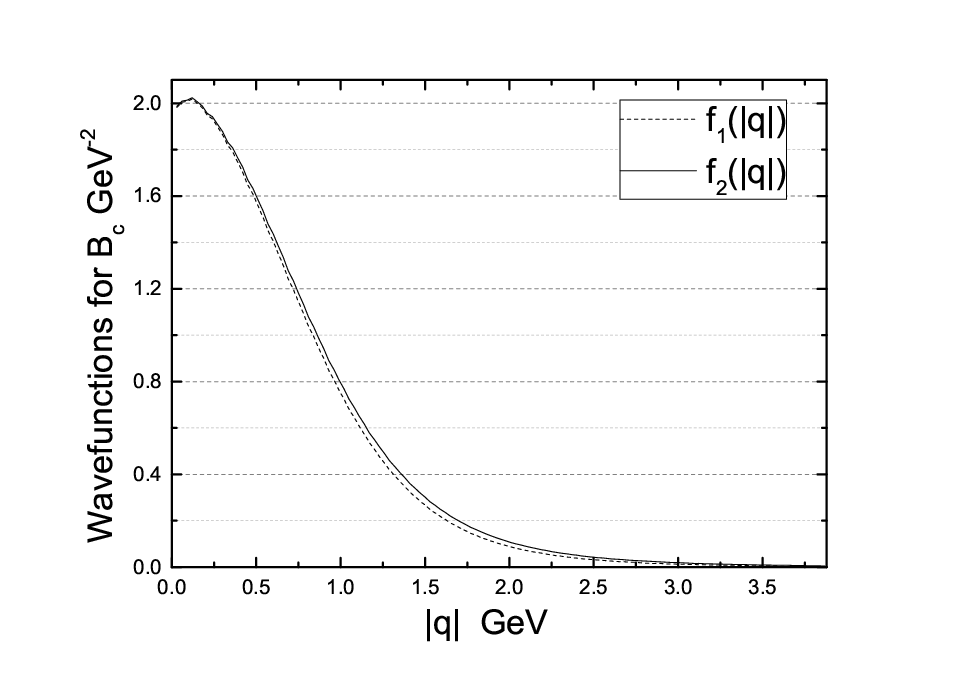
The numerical values of radial wavefunctions $f_{1}$, $f_{2}$ and eigenvalue $M$ can be obtained by solving the first two Salpeter equations in Eq. (18). To show the numerical results of wavefunctions explicitly, we plot the wavefunctions of $B_{c}$ meson in Fig. 3. According to the Eq. (17) the relativistic positive wavefunction of pseudoscalar meson $B_{c}$ in C.M.S can be written as [55]:

where the $b_{i}$s ($i=1,~2,~3,~4$) are related to the original radial wavefunctions $f_{1}$, $f_{2}$, quark masses $m_{1}$, $m_{2}$, quark energy $w_{1}$, $w_{2}$, and meson mass $M$:

Because the $X(3940)$ and $X(4160)$ mesons have the same quantum numbers as $B_{c}$, the wavefunctions of $X(3940)$ and $X(4160)$ mesons are similar to Eq. (10),

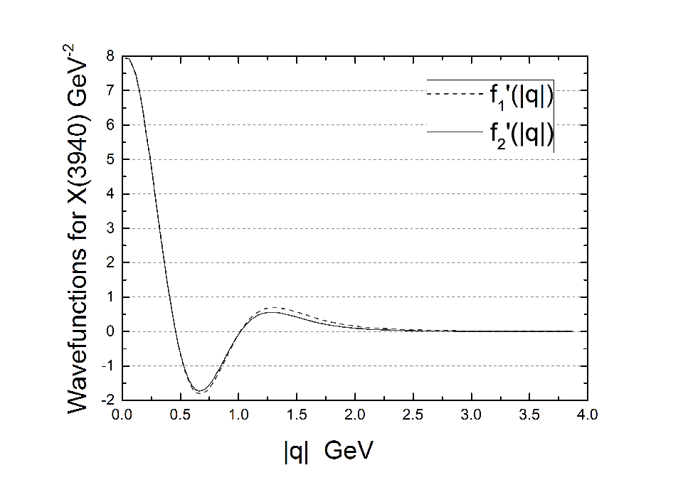
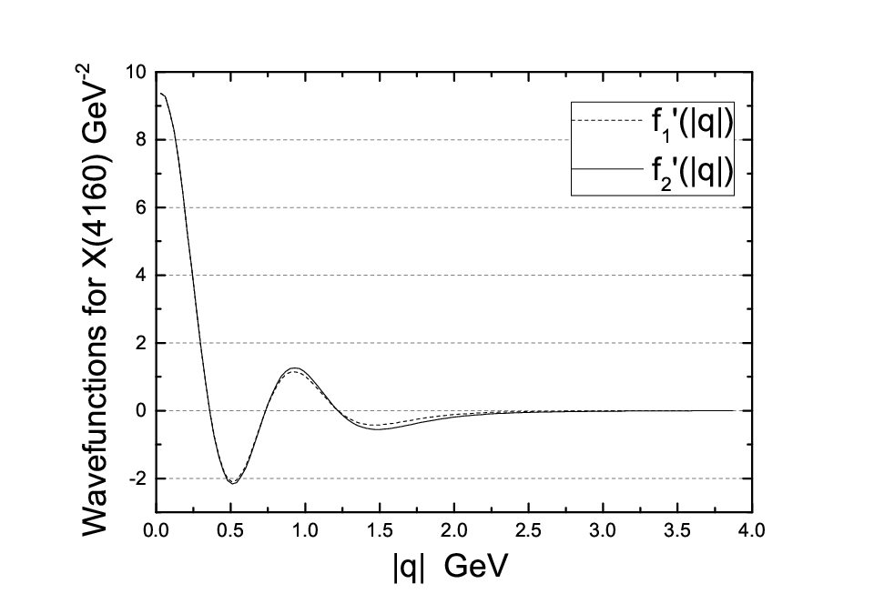
Where $M_{f}$, $P_{f}$, $f^{\prime}_{i}(\vec{q}_{f})$ are the mass, momentum and the radial wavefunctions of $X(3940)$ and $X(4160)$, respectively. $m^{\prime}_{1},m^{\prime}_{2}$ and $\omega^{\prime}_{1}=\sqrt{m_{1}^{\prime 2}+\vec{q}_{f}^{2}},\omega^{\prime}_{2}=\sqrt{m_{2}^{\prime 2}+\vec{q}_{f}^{2}}$ are the masses and the energies of quark and anti-quark in $X(3940)$ and $X(4160)$. To show the numerical results of wavefunctions explicitly, we plot the wavefunctions of $X(3940)$ and $X(4160)$ states in Fig. 4.

In order to fix Cornell potential in Eq.(22) and masses of quarks, we take these parameters: $a=e=2.7183,\lambda=0.21$ GeV², ${\Lambda}_{QCD}=0.27$ GeV, $\alpha=0.06$ GeV, $m_{b}=4.96$ GeV, $m_{c}=1.62$ GeV, $etc$ [56], which are best to fit the mass spectra of ground states $B_{c}$ and other heavy mesons. Taking these parameters to B-S equation, and solving the B-S equation numerically, we get the masses of $X(3940)$, $X(4160)$ and $B_{c}$ as: $M_{X(3940)}$=3.942 GeV, $M_{X(4160)}$=4.156 GeV, $M_{B_{c}}=6.276$ GeV.

For semileptonic decays we need to input the CKM matrix elements: $V_{cb}=0.0406$, $G_{F}=1.166\times 10^{-5}$ GeV^-2 and the life time of $B_{c}$ meson: $\tau_{B_{c}}=0.453$ps, which are taken from PDG [6]. In Section. III, we have found that the hadronic weak-current matrix element is overlapping integral over the wavefunctions of initial and final states, and the hadronic weak-current matrix element can be written as the form factors $f_{+}$ and $f_{-}$. The form factors are relate to four-momentum transfer squared $t=(P-P_{f})^{2}=M^{2}+M_{f}^{2}-2ME_{f}$ which provides the kinematic range for the semileptonic decay of $B_{c}$. It varies from $t=0$ to $t=5.45$ GeV² for the decays to $X(3940)$ and from $t=0$ to $t=4.48$ GeV² for the decays to $X(4160)$. We give the relations of $(t_{m}-t)$($t_{m}=(M-M_{f})^{2}$ is the maximum of $t$) and the form factors, which are calculated by Eq. (7) in Fig. 5. The leptonic energy spectra $\frac{d\Gamma}{\Gamma dP_{e}}$ for semileptonic $B_{c}$ decay to $X(3940)$ and $X(4160)$ are calculated by Eq. (3). The results are plot in Fig. 6. In Table. 1, we summarize the decay widths of the semileptonic $B_{c}\to X\ell^{+}\nu_{\ell}$ ($X=X(3940)$ or $X(4160)$, $\ell=e,\mu,\tau$). We have taken $\Gamma_{e}\simeq\Gamma_{\mu}$ with the massless lepton limit since the muon mass effect is negligible for these transitions with large kinematic ranges. The semileptonic decay widths of $B_{c}^{+}\to X(3940)$ are larger than $B_{c}^{+}\to X(4160)$ in Table. 1, there are two reasons: first, the former decay has larger kinematic ranges, second, there is one minus part in the wavefunctions of $X(3940)$, and there are two minus parts in the wavefunctions of $X(4160)$ in Fig. 4, after the overlapping integral in Eq. (7), much more minus parts of the wavefunctions cause the smaller result for $X(4160)$.

For the exclusive nonleptonic decay, we only consider two body decays, and another meson is light meson. The corresponding CKM matrix elements are: $V_{ud}=0.974$ and $V_{us}=0.2252$. The masses and decay constants are: $M_{\pi}=0.140$ GeV, $f_{\pi}=0.130$ GeV, $M_{\rho}=0.775$ GeV, $f_{\rho}=0.205$ GeV, $M_{K}=0.494$ GeV, $f_{K}=0.156$ GeV, $M_{K^{*}}=0.892$ GeV, $f_{K^{*}}=0.217$ GeV [6, 57], respectively. The kinematic range of nonleptonic decay is fixed value, so the form factors of $B_{c}$ nonleptonic decay are definite value. Using the form factors of $B_{c}$ nonleptonic decay and the decay constants, we show the nonleptonic decay widths which are related to the parameter $a_{1}$ in Table. 2. The results of $B_{c}$ nonleptonic decay are affected by the CKM matrix elements, so the results of light mesons $\pi,\rho$ are larger than the ones of light mesons $K,K^{*}$ in Table. 2, respectively.

In order to compare the numerical values of semileptonic and nonleptonic decays, we show the branching ratios of semileptonic and nonleptonic $B_{c}$ with $a_{1}=1.14$ [49, 50] in Table. 3. We find that the central value results of $B_{c}^{+}\to$ $X(3940)$$e^{+}\bar{\nu}_{e}$ and $B_{c}^{+}\to X(3940)\tau^{+}\bar{\nu}_{\tau}$ are less than Ref. [12]. But considering the errors of results, our results are in accordance with ones of Ref. [12]. If we compare $B_{c}\to$$X(3940)$, $X(4160)$ in this paper with $B_{c}$ decays to $\eta_{c}(1S)$ in literatures, for example in Ref. [18, 19, 41], our results are almost two order smaller than the results of $B_{c}$ decay to $\eta_{c}(1S)$. there are two reasons, one reason is that the $B_{c}\to$$X(3940)$, $X(4160)$ have small kinematic ranges, another one is that the wavefunctions have some minus parts in $X(3940)$, and $X(4160)$. Because the mass errors of $X(3940)$ and $X(4160)$ are still large, the widths and branching ratios of $B_{c}$ weak decays to $X(3940)$ and $X(4160)$ are influenced by the masses of $X(3940)$ and $X(4160)$, we plot the relations of the branching ratios of $B_{c}$ weak decays to $X(3940)$ and $X(4160)$ to the masses of $X(3940)$ and $X(4160)$ in Fig. 7. The relations of the branching ratios to the masses of $X(3940)$ and $X(4160)$ are linear. The branching ratios decrease with the increase of the masses of $X(3940)$ and $X(4160)$.

In conclusion, considering $X(3940)$ and $X(4160)$ as $\eta_{c}(3S)$ and $\eta_{c}(4S)$ states, we study the semileptonic and nonleptonic $B_{c}$ decays to $X(3940)$ and $X(4160)$ by the improved B-S method. The corresponding decay form factors are calculated and the corresponding decay widths and branching ratios are obtained. The exclusive decay widths and branching ratios are very small, because of the minus value in the wavefunctions. But now the Large Hadron Collider (LHC) will produce as much as $5\times 10^{10}$ $B_{c}$ events per year [42, 43], if we can observe the sufficient events, some channels will provide us a sizable ratios, and may be we will detect the productions of $X(3940)$ and $X(4160)$ in $B_{c}$ exclusive weak semileptonic and nonleptonic decay. That will provide us a new way to observe the $X(3940)$ and $X(4160)$ in the future.

References

- [1] K. Abe , Belle Collaboration, 89, 142001(2003).
- [2] S. K. Choi , Belle Collaboration, 91, 262001(2003).
- [3] S. Uehara , Belle Collaboration, 104, 092001(2010).
- [4] K. Abe , Belle Collaboration, 98, 082001(2007).
- [5] P. Pakhlov , Belle Collaboration, 100, 202001(2008).
- [6] K. A. Olive ., (Partile Data Group), 38, 090001(2015).
- [7] X. Liu, 59, 3815(2014).
- [8] H. X. Chen, W. Chen, X. Liu and S. L. Zhu, , 639 1(2016).
- [9] S. L. Olsen, 10, 101401(2015).
- [10] B. Q. Li and K. T. Chao, 79, 094004(2009).
- [11] H. C. Kim, K. S. Kim, M. K. Cheoun, D. Jido and M. Oka, arXiv:1602.07540 [hep-ph].
- [12] Y. M. Wang and C. D. Lu, 77, 054003(2008).
- [13] Z. G. He and B. Q. Li, 693, 36–43(2010).
- [14] R. L. Zhu, 92, 074017(2015).
- [15] L. P. He, D. Y. Chen, X. Liu and T. Matsuki, 74, 3028(2014).
- [16] Y. C. Yang, Z. R. Xia and J. L. Ping, D 81, 094003 (2010).
- [17] H. Wang, Z. Z. Yan and J. L. Ping, C 75, 196 (2015).
- [18] C. H. Chang, and Y. Q. Chen, 49, 3399(1994).
- [19] C. H. Chang and Y. Q. Chen, 46, 3845 (1992).
- [20] M. Beneke and G. Buchalla, 53, 4991 (1996).
- [21] J. F. Liu and K. T. Chao, 56, 4133 (1997).
- [22] Y. S. Dai and D. S. Du, 9, 557 (1999).
- [23] D. Ebert, R. N. Faustov and V. O. Galkin, 82, 034019 (2010).
- [24] D. Ebert, R. N. Faustov and V. O. Galkin, 82, 034032 (2010).
- [25] D. Ebert, R. N. Faustov and V. O. Galkin, 68, 094020 (2003).
- [26] D. Ebert, R. N. Faustov and V. O. Galkin, 32, 29 (2003).
- [27] D. Ebert, R. N. Faustov and V. O. Galkin, 67, 014027 (2003).
- [28] M. A. Ivanov, J. G. Krner and P. Santorelli, , 63, 074010 (2001).
- [29] M. A. Ivanov, J. G. Krner and P. Santorelli, , 73, 054024 (2006).
- [30] M. A. Ivanov, J. G. Krner and P. Santorelli, , 71, 094006, (2005), 75, 019901, (2007).
- [31] M. A. Ivanov, J. G. Krner and O. N. Pakhomova, 555, 189 (2003)
- [32] X. X. Wang, W. Wang and C. D. Lu, 79, 114018 (2009).
- [33] W. Wang, Y. L. Shen and C. D. Lu, 79, 054012 (2009).
- [34] X. Liu and Z. J. Xiao, 81, 074017 (2010).
- [35] Z. H. Wang, G. L. Wang and C. H. Chang, 39, 015009(2012).
- [36] Z. H. Wang, G. L. Wang, H. F. Fu and Y. Jiang, 27, 1250049(2012).
- [37] H. F. fu, Y. Jiang, C. S. Kim and G. L. Wang, 1106, 015(2011).
- [38] W. L. Ju, G. L. Wang, H. F. Fu, T. H. Wang and Y, Jiang, 1404, 065(2014).
- [39] W. L. Ju, G. L. Wang, H. F. Fu, Z. H. Wang and Y. Li, 1509, 171(2015).
- [40] W. L. Ju, T. H. Wang, Y. Jiang, H. Yuan and G. L. Wang, 43, 045004(2016).
- [41] C. H. Chang, H. F. Fu, G. L. Wang and J. M. Zhang, 58, 071001(2015).
- [42] N. Brambilla ., CERN Yellow Report, CERN-2005-005, and references therein.
- [43] N. Brambilla , 71, 1534 (2011).
- [44] P. Maris and C. D. Roberts, 56, 3369 (1997).
- [45] P. Maris, C. D. Roberts and P. C. Tandy, 420, 267 (1998).
- [46] M. A. Ivanov, Yu. L. Kalinovsky, P. Maris and C. D. Roberts, 57 1991(1998).
- [47] B. El-Bennich, M. A. Ivanov and C. D. Roberts, 83 025205 (2011).
- [48] C. H. Chang, J. K. Chen and G. L. Wang, 46, 467(2006).
- [49] G. Buchalla, A. J. Buras and M. E. Lautenbacher, 68, 1125(1996).
- [50] A. Ali, J. Chay. C. Greub and P.ko, 424, 161(1998).
- [51] M. Bauer, B. Stech and M. Wirbel, 34, 103(1987).
- [52] G. Cvetic, C. S. Kim, G. L. Wang and Wuk Namgung, , 596, 84(2004).
- [53] G.L. Wang, , 633, 492(2006).
- [54] S. Mandelstam, 233, 248(1955).
- [55] C. S. Kim, G. L. Wang, 584, 285(2004).
- [56] C. H. Chang and G. L. Wang, 53, 2005(2010).
- [57] P. Ball and R. Zwicky, 71, 014029 (2005).
- [58] E.E. Salpeter and H.A. Bethe, 84, 1232(1951).
- [59] C. F. Qiao, H. W. Huang and K. T Zhao, 54, 2273 (1996).
- [60] C. F. Qiao, H. W. Huang and K. T Zhao, 60, 094004 (1999).
- [61] D. Ebert, R. N. Faustov and V. O. Galkin, 62, 034014 (2000).
- [62] E.E. Salpeter, 87, 328(1952).