跳到论文正文
W Papers独立论文阅读器 arXiv:1605.09083 论文正文 计算阅读时间 · 0%
引用这篇论文根据当前论文元数据生成,正式投稿前建议核对。


License: arXiv.org perpetual non-exclusive license
arXiv:1605.09083v1 [math.PR] 30 May 2016

Projections of planar Mandelbrot measuresThanks:  2010 Mathematics Subject Classification: 28A78, 28A80, 60F10, 60G42, 60G57, 60K40

Julien Barral Address: LAGA (UMR 7539), Département de Mathématiques, Université Paris 13 (Sorbonne-Paris-Cité), 99 avenue Jean-Baptiste Clément , 93430 Villetaneuse, France, and DMA (UMR 8553), Ecole Normale Supérieure, 45 rue d’Ulm, 75005 Paris, France Email address: barral@math.univ-paris13.fr and De-Jun Feng Address:  Department of Mathematics
The Chinese University of Hong Kong
Shatin, Hong Kong
Email address: djfeng@math.cuhk.edu.hk
Abstract.

Let μ\mu be a planar Mandelbrot measure and π∗​μ\pi_{*}\mu its orthogonal projection on one of the main axes. We study the thermodynamic and geometric properties of π∗​μ\pi_{*}\mu. We first show that π∗​μ\pi_{*}\mu is exactly dimensional, with dim(π∗​μ)=min⁡(dim(μ),dim(ν))\dim(\pi_{*}\mu)=\min(\dim(\mu),\dim(\nu)), where ν\nu is the Bernoulli product measure obtained as the expectation of π∗​μ\pi_{*}\mu. We also prove that π∗​μ\pi_{*}\mu is absolutely continuous with respect to ν\nu if and only if dim(μ)>dim(ν)\dim(\mu)>\dim(\nu), and find sufficient conditions for the equivalence of these measures. Our results provides a new proof of Dekking-Grimmett-Falconer formula for the Hausdorff and box dimension of the topological support of π∗​μ\pi_{*}\mu, as well as a new variational interpretation. We obtain the free energy function τπ∗​μ\tau_{\pi_{*}\mu} of π∗​μ\pi_{*}\mu on a wide subinterval [0,qc)[0,q_{c}) of ℝ+{\mathbb{R}}_{+}. For q∈[0,1]q\in[0,1], it is given by a variational formula which sometimes yields phase transitions of order larger than 1. For q>1q>1, it is given by min⁡(τν,τμ)\min(\tau_{\nu},\tau_{\mu}), which can exhibit first order phase transitions. This is in contrast with the analyticity of τμ\tau_{\mu} over [0,qc)[0,q_{c}). Also, we prove the validity of the multifractal formalism for π∗​μ\pi_{*}\mu at each α∈(τπ∗​μ′​(qc−),τπ∗​μ′​(0+)]\alpha\in(\tau_{\pi_{*}\mu}^{\prime}(q_{c}-),\tau_{\pi_{*}\mu}^{\prime}(0+)].

Key words and phrases: 
Mandelbrot measures, Hausdorff dimension, multifractals, phase transitions, large deviations, branching random walk in a random environment

1. Introduction

Mandelbrot measures are statistically self-similar measures introduced in early seventies by B. Mandelbrot in [44] as a simplified model for energy dissipation in intermittent turbulence. In ℝ2{\mathbb{R}}^{2}, such a non-trivial random measure μ\mu is built on [0,1]2[0,1]^{2} and is characterized by the equality

(1.1) μ=∑0≤i,j≤m−1Wi,j​μ(i,j)∘Si,j−1,\mu=\sum_{0\leq i,j\leq m-1}W_{i,j}\,\mu^{(i,j)}\circ S_{i,j}^{-1},

where mm is an integer ≥2\geq 2, Si,jS_{i,j} are similarity maps on ℝ2{\mathbb{R}}^{2} defined by

Si,j​(x,y)=(x+im,y+jm),S_{i,j}(x,y)=\left(\frac{x+i}{m},\frac{y+j}{m}\right),

Wi,jW_{i,j} are non-negative random variables satisfying

𝔼⁡(∑0≤i,j≤m−1Wi,j)=1{\mathbb{E}}\left(\sum_{0\leq i,j\leq m-1}W_{i,j}\right)=1

and

D:=−𝔼⁡(∑0≤i,j≤m−1Wi,j​logm⁡(Wi,j))>0,D:=-{\mathbb{E}}\left(\sum_{0\leq i,j\leq m-1}W_{i,j}\log_{m}(W_{i,j})\right)>0,

μ(i,j)\mu^{(i,j)} are independent copies of μ\mu, which are also independent of the weights Wi,jW_{i,j}.

The topological support of μ\mu, denoted by KK, is a statistically self-similar limit set so that

K=⋃0≤i,j≤m−1Wi,j>0Si,j​(Ki,j),K=\bigcup_{\begin{subarray}{c}0\leq i,j\leq m-1\\ W_{i,j}>0\end{subarray}}S_{i,j}(K_{i,j}),

where Ki,jK_{i,j} are independent copies of KK.

The fine geometric properties of μ\mu were initially studied by Mandelbrot himself in [44, 43], as well as by Kahane and Peyrière in [37]. It was established that μ\mu is exactly DD-dimensional, i.e. the local dimension of μ\mu equals DD on a set of full μ\mu-measure. Moreover, a statistical description of the mass distribution of μ\mu at small scales was given by Mandelbrot by using large deviations properties of the branching random walk naturally associated with μ\mu.

On the other hand, the topological and measure theoretic properties of KK have been studied intensively [45, 53, 12, 18, 22, 31, 19, 25, 7, 59, 20, 48, 54, 55, 26, 52].

Mandelbrot measures, as well as self-similar measures and Gibbs measures, are typical objects illustrating the multifractal formalism, which emerged in the middle of the eighties from turbulence theory [30] and hyperbolic dynamical systems [32, 14], in order to describe geometrically at small scales the distribution of a measure, or the Hölder singularities of a function; this formalism can be viewed as a geometric counterpart of large deviations theory. For measures, it can be defined as follows.

If (X,d)(X,d) is a locally compact metric space and μ\mu is a positive and finite compactly supported measure, denoting its topological support as supp⁡(μ)\mathrm{supp}(\mu), the LqL^{q}-spectrum of μ\mu is a kind of free energy concave function defined by

τμ:q∈ℝ↦lim infr→0+logsup{∑iμ(B(xi,r))q}log⁡(r),\tau_{\mu}:q\in{\mathbb{R}}\mapsto\liminf_{r\to 0+}\frac{\log\sup\Big\{\sum_{i}\mu(B(x_{i},r))^{q}\Big\}}{\log(r)},

where the supremum is taken over all the centered packings of supp⁡(μ)\mathrm{supp}(\mu) by closed balls of radius rr. If (X,d)(X,d) possesses the Besicovitch property (like Euclidean ℝd{\mathbb{R}}^{d} or any symbolic space endowed with the standard metric), for α∈ℝ\alpha\in{\mathbb{R}} one always has (see e.g. [9, 51, 38])

dimHE⁡(μ,α)≤τμ∗​(α):=inf{α​q−τμ​(q):q∈ℝ},\dim_{H}E(\mu,\alpha)\leq\tau_{\mu}^{*}(\alpha):=\inf\{\alpha q-\tau_{\mu}(q):q\in{\mathbb{R}}\},

where

E⁡(μ,α)={x∈supp⁡(μ):limr→0+log⁡(μ⁡(B⁡(x,r)))log⁡(r)=α},E(\mu,\alpha)=\left\{x\in\mathrm{supp}(\mu):\lim_{r\to 0+}\frac{\log(\mu(B(x,r)))}{\log(r)}=\alpha\right\},

here dimH\dim_{H} stands for the Hausdorff dimension, and we adopt the convention that

dimH∅=−∞.\dim_{H}\emptyset=-\infty.

One says that the multifractal formalism holds for μ\mu at α\alpha if dimHE⁡(μ,α)=τμ∗​(α)\dim_{H}E(\mu,\alpha)=\tau_{\mu}^{*}(\alpha), and one says that it holds for μ\mu if this equality holds for all α\alpha, i.e. the Hausdorff spectrum α↦dimHE⁡(μ,α)\alpha\mapsto\dim_{H}E(\mu,\alpha) and τμ\tau_{\mu} form a Legendre pair. Furthermore, one says that there is kk-th order phase transition at qq for μ\mu if τμ\tau_{\mu} has a (k−1)(k-1)-th order derivative but no kk-th order derivative at qq.

In this paper we will investigate the multifractal structure of the orthogonal projections of a Mandelbrot measure μ\mu on the horizontal and vertical axes, and its relation with that of μ\mu. For this purpose, we recall that under mild assumptions, defining for q∈ℝq\in{\mathbb{R}}

T(q)=−logm∑0≤i,j≤m−1𝔼(𝟏{Wi,j>0}Wi,jq),T(q)=-\log_{m}\sum_{0\leq i,j\leq m-1}\mathbb{E}(\mathbf{1}_{\{W_{i,j}>0\}}W_{i,j}^{q}),

one has τμ=T\tau_{\mu}=T, hence τμ\tau_{\mu} is analytic, on the interval {q∈ℝ:T∗​(T′​(q))≥0}\{q\in{\mathbb{R}}:T^{*}(T^{\prime}(q))\geq 0\} (see Section 2.2).

In our study of projections of μ\mu, we will consider the range q≥0q\geq 0 for the LqL^{q}-spectrum. This restriction is often met in the geometric study of measures obtained via projection schemes, like self-similar measures obtained as projections of Bernoulli products on self-similar sets satisfying the weak separation condition (see e.g. [29] and the references therein) or self-affine measures obtained as projections of Bernoulli products on almost all the attractors associated with a given finite collection of contractive linear maps [24, 6].

The case of orthogonal projections πℓ∗​μ{\pi_{\ell}}_{*}\mu of μ\mu on almost every line ℓ\ell passing through the origin is essentially similar to that of Gibbs measures treated in [5]. In this case, due to Mastrand projection theorem, one is naturally led to consider the case where D≤1D\leq 1, for otherwise the projection of μ\mu is absolutely continuous with respect to Lebesgue measure and it is hard to say more about the multifractality in general. Then, since D≤1D\leq 1, the dimension of the projection is still DD, and there are two possible behaviors in terms of the LqL^{q}-spectrum. If dimHK≤1\dim_{H}K\leq 1 as well, then τπℓ∗​μ=τμ\tau_{{\pi_{\ell}}_{*}\mu}=\tau_{\mu} on the interval [0,q2][0,q_{2}], where q2q_{2} is defined by τμ​(q2)=2\tau_{\mu}(q_{2})=2 (notice that q2≥3q_{2}\geq 3 due to the concavity of τμ\tau_{\mu} and the facts that τμ​(1)=0\tau_{\mu}(1)=0 and τμ(0)≥−dimHsupp(μ)=−1\tau_{\mu}(0)\geq-\dim_{H}\mathrm{supp}(\mu)=-1 in this case). If dimHK>1\dim_{H}K>1, there is a second order phase transition at the unique q~∈[0,1]\widetilde{q}\in[0,1] at which τμ∗​(τμ′​(q~))=1\tau_{\mu}^{*}(\tau_{\mu}^{\prime}(\widetilde{q}))=1; more precisely, the LqL^{q}-spectrum τπℓ∗​μ\tau_{{\pi_{\ell}}_{*}\mu} is analytic over (0,q~)(0,\widetilde{q}) and (q~,q2)(\widetilde{q},q_{2}) but not twice differentiable at q~\widetilde{q}; specifically, it is linear on [0,q~][0,\widetilde{q}] and equals τμ\tau_{\mu} on [q~,q2][\widetilde{q},q_{2}]. Also, the multifractal formalism is valid at any α∈τπℓ∗​μ′​([0,q2])\alpha\in\tau_{{\pi_{\ell}}_{*}\mu}^{\prime}([0,q_{2}]). It is worth mentioning that the preservation of the LqL^{q}-spectrum over [1,q2][1,q_{2}] is a fact valid for any measure (see [35, 2]).

The situation is significantly different with the main axes. At first, it is worth noticing that for a Gibbs measure associated with a Hölder potential on the unit square, e.g. for the self-similar measures obtained when the weights Wi,jW_{i,j} are constant, its projection on any of the main directions is still a Gibbs measure of this kind [13], so no special new phenomenon appears related to its multifractal nature. Things turn out to be more interesting with (random) Mandelbrot measures.

Denote by π\pi the orthogonal projection on one of the main axes. It is known (Dekking and Grimmett [18], Falconer [22]), that dimHπ⁡(K)\dim_{H}\pi(K) in general differs from the typical value obtained by Mastrand’s projection theorem when one projects on almost every line. Instead of being equal to min⁡(dimHK,1)\min(\dim_{H}K,1), dimHπ⁡(K)\dim_{H}\pi(K) is given by a variational formula: denoting Ni=#⁡{0≤j≤m−1:Wi,j>0}N_{i}=\#\{0\leq j\leq m-1:W_{i,j}>0\}, one has

(1.2) dimHπ⁡(K)=inf0≤h≤1log⁡∑i=0m−1m⁡𝔼​(Ni)h.\dim_{H}\pi(K)=\inf_{0\leq h\leq 1}\log_{m}\sum_{i=0}^{m-1}{\mathbb{E}}(N_{i})^{h}.

Moreover, this dimension equals the box counting dimension of π⁡(K)\pi(K). It turns out that understanding the geometric structure of the projection π∗​μ\pi_{*}\mu of the Mandelbrot measure μ\mu heavily relies on its expectation, which is the Bernoulli product measure ν\nu associated with the probability vector (pi=∑j=0m−1𝔼⁡(Wi,j))0≤i≤m−1\left(p_{i}=\sum_{j=0}^{m-1}{\mathbb{E}}(W_{i,j})\right)_{0\leq i\leq m-1}, for which it is known that

τν​(q)=−log⁡∑0≤i≤m−1pi>0m⁡piq.\tau_{\nu}(q)=-\log_{m}\sum_{\begin{subarray}{c}0\leq i\leq m-1\\ p_{i}>0\end{subarray}}p_{i}^{q}.

In this paper, we show (Theorems 3.1 and 3.2) that when μ≠0\mu\neq 0, π∗​μ\pi_{*}\mu is exactly dimensional with dim(π∗​μ)=dim(μ)=D\dim(\pi_{*}\mu)=\dim(\mu)=D if and only if dim(μ)≤dim(ν)\dim(\mu)\leq\dim(\nu), in which case π∗​μ\pi_{*}\mu is singular with respect to ν\nu, while if dim(μ)>dim(ν)\dim(\mu)>\dim(\nu) then π∗​μ\pi_{*}\mu is absolutely continuous with respect to ν\nu. We also find sufficient conditions for the two measures to be equivalent. Exact dimensionality and “dimension conservation properties” of projections of Mandelbrot measures on all the lines have already been established in [26]; however, the result of [26] is not quantitative, whilst for the main axes we provide the precise values for the dimensions, which differ from those given by Mastrand’s theorem for almost every line when ν\nu is not the Lebesgue measure. Also, as a consequence of Theorem 3.2 we get a new variational interpretation of Dekking-Grimmett-Falconer formula for dimHπ⁡(K)\dim_{H}\pi(K) (Corollary 3.4).

Regarding the multifractal analysis (Theorem 3.6), for q≥1q\geq 1 we prove that

τπ∗​μ​(q)=min⁡(τμ​(q),τν​(q))\tau_{\pi_{*}\mu}(q)=\min(\tau_{\mu}(q),\tau_{\nu}(q))

on a non-trivial interval [1,q~c)[1,\widetilde{q}_{c}). This fact is a source of first order phase transitions when the graphs of τν\tau_{\nu} and TT cross each other transversally. For 0<q≤10<q\leq 1, we prove that τπ∗​ν\tau_{\pi_{*}\nu} is given by the following variational formula:

τπ∗​μ(q)=−inf{logm∑i=0m−1(∑j=0m−1𝔼(Wi,js))q/s:q≤s≤1},\tau_{\pi_{*}\mu}(q)=\displaystyle-\inf\left\{\log_{m}\sum_{i=0}^{m-1}\left(\sum_{j=0}^{m-1}{\mathbb{E}}(W_{i,j}^{s})\right)^{q/s}:q\leq s\leq 1\right\},

which converges to the value of dimHπ⁡(K)\dim_{H}\pi(K) given by (1.2) as qq tends to 00. The function τπ∗​μ\tau_{\pi_{*}\mu} is differentiable over [0,1][0,1]. It coincides with τμ​(q)\tau_{\mu}(q) when the infimum is attained at s=qs=q and τν​(q)\tau_{\nu}(q) when it is attained at s=1s=1. Otherwise, the infimum is attained at a unique s⁡(q)∈(q,1)s(q)\in(q,1), and this property holds on a neighborhood of qq over which by definition of s⁡(q)s(q) one has τπ∗​μ​(q)>max⁡(τμ​(q),τν​(q))\tau_{\pi_{*}\mu}(q)>\max(\tau_{\mu}(q),\tau_{\nu}(q)). These possible changes of analytic expressions lead to phase transitions of orders greater than or equal to 2. In particular, each transversal crossing of the graphs of τν\tau_{\nu} and TT gives rise to such a phase transition.

We also verify the validity of the multifractal formalism over (τπ∗​μ′​(qc−),τπ∗μ′​(0+)](\tau_{\pi_{*}\mu}^{\prime}(q_{c}-),\tau_{\pi*\mu}^{\prime}(0+)]. When applied to the so-called branching measure on KK, our result yields a partial multifractal classification of the asymptotic number of squares of a given generation necessary to cover the fibers π−1​({x})\pi^{-1}(\{x\}), x∈π⁡(K)x\in\pi(K) (see Corollary 10.1).

Let us finally mention that Mandelbrot martingales in various Bernoulli random environments play an important role in our study.

The paper is organized as follows. We will work with Mandelbrot measures on the symbolic space {0,…,m−1}ℕ×{0,…,m−1}ℕ\{0,\ldots,m-1\}^{{\mathbb{N}}}\times\{0,\ldots,m-1\}^{{\mathbb{N}}}, for this offers a simpler framework to expose ideas and techniques. We explain in Appendix D the general simple principle which makes it possible to transfer the results to the Euclidean case. In Section 2 we recall basic facts from multifractal formalism, as well as the formal definition of Mandelbrot measures and a precise known result for their multifractal analysis. In Section 3 we present in complete rigor our main results in this symbolic context, while Section 4 contains comments and examples related to phase transitions. Section 5 provides the proof of our results related to the dimension of the projected measures, as well as the new variational interpretation of the Hausdorff dimension of their topological support. Sections 6 to 8 provide the proof of Theorem 3.6 about the multifractal analysis of the projection. Specifically, Section 6 deals with the differentiability property of the function identified to be the LqL^{q}-spectrum of π∗​μ\pi_{*}\mu, Section 7 exhibits the sharp lower bound for the LqL^{q}-spectrum, and Section 8 deals both with the sharp upper bound for the LqL^{q}-spectrum and the Hausdorff spectrum. Sections 5, 7 and 8 use moments estimates developed in Section 9 for quantities related to Mandelbrot martingales in Bernoulli environments, as well as other basic results gathered in the Appendix.

2. Preliminaries on multifractal formalism and Mandelbrot measures

Throughout this paper, we use ℕ{\mathbb{N}} to denote the set of natural numbers, i.e. ℕ={1,2,…}{\mathbb{N}}=\{1,2,\ldots\}. Let us first restate the multifractal formalism in this context.

2.1. Multifractal formalism on symbolic spaces

Let m≥2m\geq 2 be an integer. For n≥0n\geq 0 let Σn={0,…,m−1}n\Sigma_{n}=\{0,\ldots,m-1\}^{n}. By convention, Σ0\Sigma_{0} consists of the empty word ϵ\epsilon. Then define Σ∗=⋃n≥0Σn\Sigma_{*}=\bigcup_{n\geq 0}\Sigma_{n}, (Σ×Σ)∗=⋃n≥0(Σn×Σn)(\Sigma\times\Sigma)_{*}=\bigcup_{n\geq 0}(\Sigma_{n}\times\Sigma_{n}), and Σ={0,…,m−1}ℕ\Sigma=\{0,\ldots,m-1\}^{\mathbb{N}}. The sets Σ∗\Sigma_{*} and (Σ×Σ)∗(\Sigma\times\Sigma)_{*} act in the standard way by concatenation on Σ∗∪Σ\Sigma_{*}\cup\Sigma and (Σ×Σ)∗∪(Σ×Σ)(\Sigma\times\Sigma)_{*}\cup(\Sigma\times\Sigma) respectively. We denote by σ\sigma the standard left shift operation on Σ∗∪(Σ×Σ)\Sigma_{*}\cup(\Sigma\times\Sigma). The length of a word w∈Σ∗w\in\Sigma_{*}, i.e. its number of letters, is denoted as |w||w|.

For x=x1⋯xp⋯∈Σx=x_{1}\cdots x_{p}\cdots\in\Sigma, set x|n=x1⋯xnx_{|n}=x_{1}\cdots x_{n} if n≥1n\geq 1 and ϵ\epsilon if n=0n=0. For u∈Σ∗u\in\Sigma_{*}, set [u]={x∈Σ:x||u|=u}[u]=\{x\in\Sigma:x_{||u|}=u\}.

The set Σ\Sigma is endowed with the standard metric distance

d(x,x′)=m−sup{n:x|n=x′|n},d(x,x^{\prime})=m^{-\sup\left\{n:\,x_{|n}=x^{\prime}_{|n}\right\}},

and Σ×Σ\Sigma\times\Sigma is endowed with the distance d⁡((x,y),(x′,y′))=max⁡(d⁡(x,x′),d⁡(y,y′))d((x,y),(x^{\prime},y^{\prime}))=\max(d(x,x^{\prime}),d(y,y^{\prime})).

Given a positive and finite Borel measure ρ\rho on Σ\Sigma or Σ×Σ\Sigma\times\Sigma, its topological support, i.e. the smallest closed set carrying the whole mass of μ\mu is denoted as supp⁡(ρ)\mathrm{supp}(\rho), and its lower and upper local dimensions at x∈supp⁡(ρ)x\in\mathrm{supp}(\rho) are defined as

dim¯loc​(ρ,x)=lim infn→∞log(ρ([x|n]))(−n​log⁡(m))anddim¯loc​(ρ,x)=lim supn→∞log(ρ([x|n]))(−n​log⁡(m))\underline{\dim}_{\rm loc}(\rho,x)=\displaystyle\liminf_{n\to\infty}\frac{\log(\rho([x_{|n}]))}{(-n\log(m))}\quad\text{and}\quad\overline{\dim}_{\rm loc}(\rho,x)=\displaystyle\limsup_{n\to\infty}\frac{\log(\rho([x_{|n}]))}{(-n\log(m))}

respectively. Let

dim¯H​(ρ)\displaystyle\underline{\dim}_{H}(\rho) =inf{dimHE:ρ⁡(E)>0​ and E is a Borel set}​and\displaystyle=\inf\{\dim_{H}E:\,\rho(E)>0\mbox{ and $E$ is a Borel set}\}\;\text{and}
dim¯P​(ρ)\displaystyle\quad\overline{\dim}_{P}(\rho) =inf{dimPE:ρ⁡(E)=‖ρ‖​ and E is a Borel set},\displaystyle=\inf\{\dim_{P}E:\rho(E)=\|\rho\|\mbox{ and $E$ is a Borel set}\},

where dimPE\dim_{P}E stands for the packing dimension of EE (see e.g. [46]) and ‖ρ‖\|\rho\| stands for the total mass of ρ\rho .

It is well known that (see e.g. [15, 16])

dim¯H​(ρ)\displaystyle\underline{\dim}_{H}(\rho) =sup{s:dim¯loc​(ρ,x)≥s​ for ρ-almost every x}​and\displaystyle=\sup\{s:\;\underline{\dim}_{\rm loc}(\rho,x)\geq s\mbox{ for $\rho$-almost every $x$}\}\;\mbox{and}
dim¯P​(ρ)\displaystyle\overline{\dim}_{P}(\rho) =inf{s:dim¯loc​(ρ,x)≤s​ for ρ–almost every x};\displaystyle=\inf\{s:\;\overline{\dim}_{\rm loc}(\rho,x)\leq s\mbox{ for $\rho$--almost every $x$}\};

when these two dimensions coincide, one says that ρ\rho is exactly dimensional and writes dim(ρ)\dim(\rho) for the common value.

The LqL^{q}-spectrum of ρ\rho is the mapping τρ:ℝ→ℝ∪{−∞}\tau_{\rho}:\;{\mathbb{R}}\to{\mathbb{R}}\cup\{-\infty\} given by

τρ(q)=lim infn→∞−1nlogm∑w∈Sn𝟏{ρ([w])>0}ρ([w])q(q∈ℝ),\tau_{\rho}(q)=\liminf_{n\to\infty}\frac{-1}{n}\log_{m}\sum_{w\in S_{n}}\mathbf{1}_{\{\rho([w])>0\}}\rho([w])^{q}\quad(q\in{\mathbb{R}}),

where SnS_{n} stands for Σn\Sigma_{n} or Σn×Σn\Sigma_{n}\times\Sigma_{n}. It is well known that (cf. [49])

τρ′​(1+)≤dim¯H​(ρ)≤dim¯P​(ρ)≤τρ′​(1−).\tau_{\rho}^{\prime}(1+)\leq\underline{\dim}_{H}(\rho)\leq\overline{\dim}_{P}(\rho)\leq\tau_{\rho}^{\prime}(1-).

For all α∈ℝ\alpha\in{\mathbb{R}}, set

E¯​(ρ,α)\displaystyle\underline{E}(\rho,\alpha) ={x∈supp⁡(ρ):dim¯loc​(ρ,x)=α},\displaystyle=\{x\in\mathrm{supp}(\rho):\underline{\dim}_{\rm{loc}}(\rho,x)=\alpha\},
E¯​(ρ,α)\displaystyle\overline{E}(\rho,\alpha) ={x∈supp⁡(μ):dim¯loc​(ρ,x)=α}\displaystyle=\{x\in\mathrm{supp}(\mu):\overline{\dim}_{\rm{loc}}(\rho,x)=\alpha\}

and

E⁡(ρ,α)=E¯​(ρ,α)∩E¯​(ρ,α).E(\rho,\alpha)=\underline{E}(\rho,\alpha)\cap\overline{E}(\rho,\alpha).

Then one also always has (see e.g. [38, 51]) that

dimHE⁡(ρ,α)≤max⁡(dimHE¯​(ρ,α),dimHE¯​(ρ,α))≤τρ∗​(α),\dim_{H}E(\rho,\alpha)\leq\max(\dim_{H}\underline{E}(\rho,\alpha),\dim_{H}\overline{E}(\rho,\alpha))\leq\tau_{\rho}^{*}(\alpha),

where the Legendre transform of f:ℝ→ℝ∪{−∞}f:{\mathbb{R}}\to{\mathbb{R}}\cup\{-\infty\} is defined as

f∗:α∈ℝ↦infq∈ℝ(α​q−f⁡(q)),f^{*}:\alpha\in{\mathbb{R}}\mapsto\inf_{q\in{\mathbb{R}}}(\alpha q-f(q)),

and a negative dimension means that the set is empty. One says that the multifractal formalism holds at α\alpha if

dimHE⁡(ρ,α)=τρ∗​(α).\dim_{H}E(\rho,\alpha)=\tau_{\rho}^{*}(\alpha).

Also, if α≤τρ′​(0+)\alpha\leq\tau_{\rho}^{\prime}(0+), one has (see e.g. [38, 51])

(2.1) dimHE¯≤​(ρ,α)≤τρ∗​(α),\dim_{H}\underline{E}^{\leq}(\rho,\alpha)\leq\tau_{\rho}^{*}(\alpha),

where

E¯≤​(ρ,α)={x∈supp⁡(ρ):dim¯loc​(ρ,x)≤α}.\underline{E}^{\leq}(\rho,\alpha)=\{x\in\mathrm{supp}(\rho):\underline{\dim}_{\rm{loc}}(\rho,x)\leq\alpha\}.

2.2. Multifractal analysis of the Mandelbrot measures on Σ×Σ\Sigma\times\Sigma

Now let us formally define the Mandelbrot measures on Σ×Σ\Sigma\times\Sigma. We consider a non-negative random vector

W=(Wi,j)(i,j)∈Σ1×Σ1W=(W_{i,j})_{(i,j)\in\Sigma_{1}\times\Sigma_{1}}

whose entries are integrable. For q∈ℝq\in{\mathbb{R}} we define

(2.2) T(q)=TW(q)=−logm∑(i,j)∈Σ1×Σ1𝔼(𝟏{Wi,j>0}Wi,jq).T(q)=T_{W}(q)=-\log_{m}\sum_{(i,j)\in\Sigma_{1}\times\Sigma_{1}}\mathbb{E}(\mathbf{1}_{\{W_{i,j}>0\}}W_{i,j}^{q}).

We denote N=∑(i,j)∈Σ1×Σ1𝟏{Wi,j>0}N=\sum_{(i,j)\in\Sigma_{1}\times\Sigma_{1}}\mathbf{1}_{\{W_{i,j}>0\}}, and assume that ℙ⁡(N∈{0,1})<1\mathbb{P}(N\in\{0,1\})<1.

To build a Mandelbrot measure on Σ×Σ\Sigma\times\Sigma we assume that T⁡(1)=0T(1)=0 and consider a sequence (W⁡(u,v))(u,v)∈⋃n≥0Σn×Σn(W(u,v))_{(u,v)\in\bigcup_{n\geq 0}\Sigma_{n}\times\Sigma_{n}} of independent copies of WW, defined on a probability space (Ω,𝒜,ℙ)(\Omega,\mathcal{A},\mathbb{P}).

For each n≥1n\geq 1 let μn=μW,n\mu_{n}=\mu_{W,n} be the measure on Σ×Σ\Sigma\times\Sigma whose density with respect to the measure of maximal entropy is constant over each cylinder [u,v]:=[u]×[v][u,v]:=[u]\times[v] of generation nn and given by m2​n​Q​(u,v)m^{2n}Q(u,v), where

Q(u,v)=∏j=1nWuj,vj(u|j−1,v|j−1).Q(u,v)=\prod_{j=1}^{n}W_{u_{j},v_{j}}(u_{|j-1},v_{|j-1}).

Denote the total mass of μn\mu_{n} as YnY_{n}, i.e.

Yn=∑|u|=|v|=nQ⁡(u,v).Y_{n}=\sum_{|u|=|v|=n}Q(u,v).

By construction the sequence (Yn)n≥1(Y_{n})_{n\geq 1} is a non-negative martingale of expectation 11 with respect to the filtration (σ(W(u,v):|u|=|v|≤n−1))n≥1(\sigma(W(u,v):|u|=|v|\leq n-1))_{n\geq 1}, thus it converges to a limit, which we denote by YY.

Let Tn={(u,v)∈Σn×Σn:Q⁡(u,v)>0}T_{n}=\{(u,v)\in\Sigma_{n}\times\Sigma_{n}:Q(u,v)>0\}. The sequence (Tn)n≥1(T_{n})_{n\geq 1} represents the generations of a Galton-Watson process with offspring distribution given by that of NN. We have

Kn:=supp⁡(μn)=⋃(u,v)∈Tn[u]×[v].K_{n}:={\rm supp}(\mu_{n})=\bigcup_{(u,v)\in T_{n}}[u]\times[v].

For n≥k≥1n\geq k\geq 1 and (u,v)∈Σk×Σk(u,v)\in\Sigma_{k}\times\Sigma_{k}, the statistical self-similarity of the construction yields (μn​([u]×[v])=Q⁡(u,v)​Yn−k​(u,v)CLOSE(\mu_{n}([u]\times[v])=Q(u,v)Y_{n-k}(u,v), with (Yn−k​(u,v))(u,v)∈Σk×Σk(Y_{n-k}(u,v))_{(u,v)\in\Sigma_{k}\times\Sigma_{k}} a family of independent copies of Yn−kY_{n-k}, also independent of σ(W(u,v):|u|=|v|≤k−1)\sigma(W(u,v):|u|=|v|\leq k-1).

Consequently, with probability 1, there exists a family OPEN(Y⁡(u,v))(u,v)∈Σk×Σk,k≥1)(Y(u,v))_{(u,v)\in\Sigma_{k}\times\Sigma_{k},k\geq 1}) of copies of YY such that for each k≥1k\geq 1 and (u,v)∈Σk×Σk(u,v)\in\Sigma_{k}\times\Sigma_{k},

(2.3) limn→∞μn​([u]×[v])=Q⁡(u,v)​Y​(u,v).\lim_{n\to\infty}\mu_{n}([u]\times[v])=Q(u,v)Y(u,v).

Moreover, the random variables Y⁡(u,v)Y(u,v), (u,v)∈Σk×Σk(u,v)\in\Sigma_{k}\times\Sigma_{k}, are independent, and generate a σ\sigma-field independent of σ(W(u,v):|u|=|v|≤k−1)\sigma(W(u,v):|u|=|v|\leq k-1). By construction, this means that μn\mu_{n} weakly converges to a measure μ\mu defined by

μ⁡([u]×[v])=Q⁡(u,v)​Y​(u,v).\mu([u]\times[v])=Q(u,v)Y(u,v).

Moreover, μ\mu is positive (i.e. Y>0Y>0) with positive probability if and only if T′​(1−)>0T^{\prime}(1-)>0; and this is also equivalent to the uniform integrability of (Yn)n≥1(Y_{n})_{n\geq 1}, that is 𝔼⁡(Y)=1{\mathbb{E}}(Y)=1 ([37, 11]). From now on we assume that this condition (i.e., T′​(1−)>0T^{\prime}(1-)>0) holds; in this case, it is known (cf. [37, 36]) that the measure μ\mu, if non-degenerate, is exactly dimensional and

dim(μ)=T′(1−) almost surely on {μ≠0}.\dim(\mu)=T^{\prime}(1-)\text{ almost surely on }\{\mu\neq 0\}.

Also, the events {μ≠0}\{\mu\neq 0\} and {K:=⋂n≥1Kn≠∅}\{K:=\bigcap_{n\geq 1}K_{n}\neq\emptyset\} coincide up to a set of probability 0 over which we have K=supp⁡(μ)K=\mathrm{supp}(\mu) (see Proposition A.1 for a proof). In addition, the inequality T′​(1−)>0T^{\prime}(1-)>0 and the concavity of TT imply that T⁡(0)=−logm⁡(𝔼⁡(N))<0T(0)=-\log_{m}({\mathbb{E}}(N))<0, i.e. 𝔼⁡(N)>1{\mathbb{E}}(N)>1.

We have the following result regarding the multifractal analysis of μ\mu (see also [33, 23, 50, 47, 4] for slightly less sharp versions).

Theorem 2.1 ([1]).

Suppose that TT is finite on a neighborhood of 00 and that conditionally on N≠0N\neq 0 one has N≥2N\geq 2. Define f​(α)=T∗​(α)f(\alpha)=T^{*}(\alpha) if T∗​(α)≥0T^{*}(\alpha)\geq 0 and f⁡(α)=−∞f(\alpha)=-\infty otherwise. With probability 1, conditionally on {μ≠0}\{\mu\neq 0\}, τμ=f∗\tau_{\mu}=f^{*} and the multifractal formalism holds at all α\alpha in the domain of τμ∗=f\tau_{\mu}^{*}=f. In particular, τμ​(q)=T​(q)\tau_{\mu}(q)=T(q) at each q∈ℝq\in{\mathbb{R}} such that T∗​(T′​(q))≥0T^{*}(T^{\prime}(q))\geq 0.

Since we mainly want to focus on new phenomena associated with π∗​μ\pi_{*}\mu, we will avoid to deal with too many technicalities and discard the case when

sup{q≥1:T⁡(q)>−∞}=sup{q≥1:T∗​(T′​(q))>0}.\sup\{q\geq 1:T(q)>-\infty\}=\sup\{q\geq 1:T^{*}(T^{\prime}(q))>0\}.

Thus, when we study the validity of the multifractal formalism for π∗​μ\pi_{*}\mu, our assumptions will be:

(2.4) ∙ℙ⁡(N∈{0,1})​<1,T′​(1−)>​0;∙T​ is finite on a neighborhood of 0;∙either ∃ qc>1 such that T∗​(T′​(qc−))=0or T∗​(T′​(q))>0 for all q≥0, in which case we set qc=∞.\begin{split}&\bullet\ \mathbb{P}(N\in\{0,1\})<1,\ T^{\prime}(1-)>0;\\ &\bullet\ T\text{ is finite on a neighborhood of $0$};\\ &\bullet\ \text{either $\exists$ $q_{c}>1$ such that $T^{*}(T^{\prime}(q_{c}^{-}))=0$}\\ &\quad\;\text{or $T^{*}(T^{\prime}(q))>0$ for all $q\geq 0$, in which case we set $q_{c}=\infty$}.\end{split}

We drop the assumption that N≥2N\geq 2 when N≠0N\neq 0 because this does not affect the validity of Theorem 2.1 for the local dimensions α\alpha associated with non-negative qq by Legendre duality, and our study of π∗​μ\pi_{*}\mu we will only focus on the case q≥0q\geq 0.

3. Main results for projections of Mandelbrot measures

Throughout this section we assume that ℙ⁡(N∈{0,1})<1\mathbb{P}(N\in\{0,1\})<1 and T′​(1−)>0T^{\prime}(1-)>0. We are interested in the geometric properties of the measure π∗​μ\pi_{*}\mu, where π\pi stands for the canonical projection onto the first factor of Σ×Σ\Sigma\times\Sigma. We are also concerned with the disintegrations of μ\mu associated with the projection π\pi.

For 0≤i,j≤m−10\leq i,j\leq m-1 set

pi=∑j=0m−1𝔼⁡(Wi,j)​ and ​Vi,j={Wi,j/pi if pi>0,1/m otherwise.p_{i}=\sum_{j=0}^{m-1}{\mathbb{E}}(W_{i,j})\text{ and }V_{i,j}=\begin{cases}W_{i,j}/p_{i}&\text{ if $p_{i}>0$,}\\ {1}/{m}&\text{ otherwise.}\end{cases}

(In fact those ii for which pi=0p_{i}=0 will play no role in our study.) Then write Vi:=(Vi,j)j∈Σ1V_{i}:=(V_{i,j})_{j\in\Sigma_{1}} and define

(3.1) Ti(q)=TVi(q)=−logm∑j∈Σ1𝔼(𝟏{Vi,j>0}Vi,jq),q∈ℝ.T_{i}(q)=T_{V_{i}}(q)=-\log_{m}\sum_{j\in\Sigma_{1}}\mathbb{E}(\mathbf{1}_{\{V_{i,j}>0\}}V_{i,j}^{q}),\qquad q\in{\mathbb{R}}.

Notice that Ti​(1)=0T_{i}(1)=0 for all 0≤i≤m−10\leq i\leq m-1.

Let ν\nu stand for the Bernoulli product measure on Σ\Sigma associated with the probability vector (p0,…,pm−1)(p_{0},\ldots,p_{m-1}), that is

ν⁡([x1​…​xn])=px1​…​pxn\nu([x_{1}\ldots x_{n}])=p_{x_{1}}\ldots p_{x_{n}}

for n≥1n\geq 1 and x1,…,xn∈{0,1,…,m−1}x_{1},\ldots,x_{n}\in\{0,1,\ldots,m-1\}.

By construction we have

(3.2) m−T⁡(q)=∑i,j𝔼(𝟏{Wi,j>0}Wi,jq)=∑i,j𝟏{pi>0}piq𝔼(Vi,jq)=∑i𝟏{pi>0}piqm−Ti​(q).m^{-T(q)}=\sum_{i,j}\mathbb{E}(\mathbf{1}_{\{W_{i,j}>0\}}W_{i,j}^{q})=\sum_{i,j}\mathbf{1}_{\{p_{i}>0\}}p_{i}^{q}\mathbb{E}(V_{i,j}^{q})=\sum_{i}\mathbf{1}_{\{p_{i}>0\}}p_{i}^{q}m^{-T_{i}(q)}.

Consequently,

(3.3) T′​(1−)=∑ipi​(Ti′​(1−)−logm⁡(pi))=(∑ipi​Ti′​(1−))+dim(ν),T^{\prime}(1-)=\sum_{i}p_{i}(T^{\prime}_{i}(1-)-\log_{m}(p_{i}))=\Big(\sum_{i}p_{i}T^{\prime}_{i}(1-)\Big)+\dim(\nu),

where we recall that

dim(ν)=−∑i=0m−1pilog(pi)/log(m).\dim(\nu)=-\sum_{i=0}^{m-1}p_{i}\log(p_{i})/\log(m).

Notice that ν=𝔼⁡(π∗​μ)\nu=\mathbb{E}(\pi_{*}\mu), and recall that a direct calculation yields

τν​(q)=−log⁡∑i=0m−1m⁡piq(q∈ℝ).\tau_{\nu}(q)=-\log_{m}\sum_{i=0}^{m-1}p_{i}^{q}\quad(q\in{\mathbb{R}}).

For q∈ℝq\in{\mathbb{R}}, we denote by νq\nu_{q} the Bernoulli product measure on Σ\Sigma associated with the probability vector (p0q​mτν​(q),…,pm−1q​mτν​(q))\big(p_{0}^{q}m^{\tau_{\nu}(q)},\ldots,p_{m-1}^{q}m^{\tau_{\nu}(q)}\big).

Below we discard two trivial situations.

We first discard the case when pi=1p_{i}=1 for some 0≤i≤m−10\leq i\leq m-1, which means that the measure μ\mu is supported on a deterministic vertical line hence is a Mandelbrot measure on a line, for which the multifractal nature is analogue to that of a 1-dimensional Mandelbrot measures. For 0≤i≤m−10\leq i\leq m-1, we set

(3.4) Ni=#⁡{0≤j≤m−1:Wi,j>0}.N_{i}=\#\{0\leq j\leq m-1:W_{i,j}>0\}.

We also discard the case when Ni=1N_{i}=1 almost surely for all 0≤i≤m−10\leq i\leq m-1, which implies that π∗​μ\pi_{*}\mu is a Mandelbrot measure on a line as well.

3.1. Absolute continuity and dimension

This section gathers our results on the absolute continuity/singularity of π∗​μ\pi_{*}\mu with respect to ν=𝔼⁡(π∗​μ)\nu=\mathbb{E}(\pi_{*}\mu), and on the dimension of π∗​μ\pi_{*}\mu and its associated conditional measures in the natural disintegration of μ\mu along π∗​μ\pi_{*}\mu-almost every fiber {x}×Σ\{x\}\times\Sigma. The result on dim(π∗​μ)\dim(\pi_{*}\mu) also yields a new variational principle for dimπ⁡(K)\dim\pi(K).

Theorem 3.1.

With probability 1, conditionally on {μ≠0}\{\mu\neq 0\}:

  1. (1)

    If dim(μ)>dim(ν)\dim(\mu)>\dim(\nu), then

    • (i)

      π∗​μ\pi_{*}\mu is absolutely continuous with respect to ν\nu.

    • (ii)

      Suppose that TT is finite in a neighborhood of 11. Then the density of π∗​ν\pi_{*}\nu with respect to ν\nu is in LsL^{s} for all ss in the following non-empty set

      {s∈(1,2]:T⁡(s)>0​ and ​∑i=0m−1pi​m−Ti​(s)<1}.\left\{s\in(1,2]:\;T(s)>0\text{ and }\sum_{i=0}^{m-1}p_{i}m^{-T_{i}(s)}<1\right\}.
    • (iii)

      Suppose, moreover, that there exists c∈(0,1)c\in(0,1) such that both

      ℙ⁡(sup0≤j≤m−1Vi,j>c)=1​ and ​𝔼​(#⁡{j:Vi,j>c})>1\mathbb{P}\left(\sup_{0\leq j\leq m-1}V_{i,j}>c\right)=1\mbox{ and }\;{\mathbb{E}}(\#\{j:V_{i,j}>c\})>1

      hold for all ii such that pi>0p_{i}>0. Then ν\nu is absolutely continuous with respect to π∗​μ\pi_{*}\mu, and its density with respect to π∗​μ\pi_{*}\mu is in LsL^{s} for some s>1s>1.

  2. (2)

    If dim(μ)≤dim(ν)\dim(\mu)\leq\dim(\nu), then π∗​μ\pi_{*}\mu and ν\nu are mutually singular.

Theorem 3.2.

With probability 1, conditionally on {μ≠0}\{\mu\neq 0\}:

  1. (1)

    If dim(μ)>dim(ν)\dim(\mu)>\dim(\nu) then π∗​μ\pi_{*}\mu is exactly dimensional with dimension dim(ν)\dim(\nu); while if dim(μ)≤dim(ν)\dim(\mu)\leq\dim(\nu) and TT is finite in a neighborhood of 11, then π∗​μ\pi_{*}\mu is exactly dimensional with dimension dim(μ)\dim(\mu).

  2. (2)

    For π∗​μ\pi_{*}\mu-almost every xx, the conditional measure μx\mu^{x} is exactly dimensional with dimension dim(μ)−dim(π∗​μ)=dim(μ)−dim(ν)=∑i=0m−1pi​Ti′​(1)\dim(\mu)-\dim(\pi_{*}\mu)=\dim(\mu)-\dim(\nu)=\sum_{i=0}^{m-1}p_{i}T^{\prime}_{i}(1) if dim(μ)>dim(ν)\dim(\mu)>\dim(\nu), and dimension 0 if dim(μ)≤dim(ν)\dim(\mu)\leq\dim(\nu) and TT is finite in a neighborhood of 11.

Remark 3.3.

Recall that in [26] Falconer and Jin have already proven that with probability 1, conditionally on μ≠0\mu\neq 0, for π∗​μ\pi_{*}\mu-almost every xx one has dim(μx)=dim(μ)−dim(π∗​μ)\dim(\mu^{x})=\dim(\mu)-\dim(\pi_{*}\mu), without specifying the value of dim(π∗​μ)\dim(\pi_{*}\mu), hence of dim(μx)\dim(\mu^{x}). Here we give an alternative proof of the exact dimensionality of π∗​μ\pi_{*}\mu and find its dimension, and in the case when dim(μ)>dim(ν)\dim(\mu)>\dim(\nu), we also give an alternative proof of the exact dimensions of μx\mu^{x} and the dimension preservation dim(μ)=dim(π∗​μ)+dim(μx)\dim(\mu)=\dim(\pi_{*}\mu)+\dim(\mu^{x}). When dim(μ)≤dim(ν)\dim(\mu)\leq\dim(\nu), the exact dimensionality of μx\mu^{x} follows from [26], but our result on dim(π∗​μ)\dim(\pi_{*}\mu) yields that the dimension of μx\mu^{x} is 0. Without using the work in [26], our result on dim(π∗​μ)\dim(\pi_{*}\mu) and simple arguments would give dim¯H​(μx)=0\underline{\dim}_{H}(\mu^{x})=0.

The previous statement makes it possible to derive the dimension formula of π⁡(K)\pi(K) by using an adapted Mandelbrot measure, whilst in [22] Falconer builds statistically self-similar subsets of π⁡(K)\pi(K) of Hausdorff dimension smaller than but arbitrarily close to the value given by (1.2). The new point is the variational principle invoking Mandelbrot measures in (3.6) and the related uniqueness property.

Corollary 3.4 (Dekking-Grimmett-Falconer formula revisited).

Let

(3.5) φ:h≥0↦log⁡(∑i=0m−1𝔼​(Ni)h)/log⁡(m).\varphi:h\geq 0\mapsto\log\left(\sum_{i=0}^{m-1}{\mathbb{E}}(N_{i})^{h}\right)/\log(m).

With probability 1, conditionally on K≠∅K\neq\emptyset, we have

(3.6) dimHπ⁡(K)=dimB(π⁡(K))=inf0≤h≤1φ⁡(h)=max⁡{dim(π∗​μ′):μ′​is a Mandelbrot measure supported on K}.\begin{split}\dim_{H}\pi(K)&=\dim_{B}(\pi(K))\\ &=\inf_{0\leq h\leq 1}\varphi(h)\\ &=\max\{\dim(\pi_{*}\mu^{\prime}):\mu^{\prime}\ \text{{\rm is a Mandelbrot measure supported on $K$}}\}.\end{split}

Moreover, the maximum in (3.6) is attained at a unique point if and only if φ′​(0)≤0\varphi^{\prime}(0)\leq 0, i.e. ∑i=0m−1log⁡(𝔼⁡(Ni))≤0\sum_{i=0}^{m-1}\log({\mathbb{E}}(N_{i}))\leq 0.

Remark 3.5.

One has dimHπ⁡(K)=dimHK\dim_{H}\pi(K)=\dim_{H}K if and only if ∑i=0m−1𝔼⁡(Ni)​log⁡𝔼⁡(Ni)≤0\sum_{i=0}^{m-1}{\mathbb{E}}(N_{i})\log{\mathbb{E}}(N_{i})\leq 0, i.e. in (3.6) the infimum is attained at h=1h=1.

3.2. Multifractal formalism for π∗​μ\pi_{*}\mu

Assume (2.4) and define

q~c={qcif qc<∞ and ​τν​(qc)≥T⁡(qc)inf{q>qc:τν​(q)≥T⁡(q)} otherwise,\widetilde{q}_{c}=\begin{cases}q_{c}&\text{if $q_{c}<\infty$ and }\tau_{\nu}(q_{c})\geq T(q_{c})\\ \inf\{q>q_{c}:\tau_{\nu}(q)\geq T(q)\}&\text{ otherwise}\end{cases},

with the convention that inf∅=qc\inf\emptyset=q_{c}. Let

τ:q↦{−inf{logm∑i=0m−1𝔼(Ni)h:0≤h≤1} if ​q=0,−inf{logm∑i=0m−1piqm−qTi(s)/s:q≤s≤1} if ​0<q≤1,min⁡(τν​(q),T⁡(q)) if ​1<q<q~c​ or ​q=q~c<∞.\tau:q\mapsto\begin{cases}\displaystyle-\inf\left\{\log_{m}\sum_{i=0}^{m-1}{\mathbb{E}}(N_{i})^{h}:0\leq h\leq 1\right\}&\text{ if }q=0,\\ \displaystyle-\inf\left\{\log_{m}\sum_{i=0}^{m-1}p_{i}^{q}m^{-qT_{i}(s)/s}:q\leq s\leq 1\right\}&\text{ if }0<q\leq 1,\\ \min(\tau_{\nu}(q),T(q))&\text{ if }1<q<\widetilde{q}_{c}\text{ or }q=\widetilde{q}_{c}<\infty.\end{cases}
Theorem 3.6.

The function τ\tau is differentiable everywhere except at the possible points in (1,q~c)(1,\widetilde{q}_{c}) at which the graphs of TT and τν\tau_{\nu} cross each other transversally. Moreover,

  1. (1)

    with probability 1, conditionally on {μ≠0}\{\mu\neq 0\}, for all q∈[0,q~c)q\in[0,\widetilde{q}_{c}) we have

    (3.7) τ(q)=limn→∞−1nlogm∑|u|=n𝟏{π∗μ([u])>0}π∗μ([u])q.\tau(q)=\lim_{n\to\infty}\frac{-1}{n}\log_{m}\sum_{|u|=n}\mathbf{1}_{\{\pi_{*}\mu([u])>0\}}\pi_{*}\mu([u])^{q}.

    In particular τπ∗​μ​(q)=τ​(q)\tau_{\pi_{*}\mu}(q)=\tau(q). Also, if q~c=qc<∞\widetilde{q}_{c}=q_{c}<\infty, we have τπ∗​μ​(q)=q​T′​(qc−)\tau_{\pi_{*}\mu}(q)=qT^{\prime}(q_{c}-) for q>qcq>q_{c}.

  2. (2)

    If α∈(τ′​(q~c−),τ′​(0+)]\alpha\in(\tau^{\prime}(\widetilde{q}_{c}-),\tau^{\prime}(0+)], with probability 1, conditionally on {μ≠0}\{\mu\neq 0\}, the multifractal formalism holds at α\alpha.

Remark 3.7.

Notice that when qc<∞q_{c}<\infty, the equality τν​(qc)=T⁡(qc)\tau_{\nu}(q_{c})=T(q_{c}) cannot hold if τν′​(qc)≤T′​(qc−)\tau_{\nu}^{\prime}(q_{c})\leq T^{\prime}(q_{c}-), for this would imply that τν∗​(τν′​(qc))≤T∗​(T′​(qc−))=0\tau_{\nu}^{*}(\tau_{\nu}^{\prime}(q_{c}))\leq T^{*}(T^{\prime}(q_{c}-))=0, while τν∗∘τν′\tau_{\nu}^{*}\circ\tau_{\nu}^{\prime} is always positive over ℝ{\mathbb{R}}.

Remark 3.8.

The same conclusion as in (3.7) and Theorem 3.6(2) holds if we replace π∗μ([x|n])\pi_{*}\mu([x_{|n}]) by π∗μn([x|n])\pi_{*}\mu_{n}([x_{|n}]) in the definition of the level sets E⁡(π∗​μ,α)E(\pi_{*}\mu,\alpha).

Remark 3.9.

(1) One has τ=T=τν\tau=T=\tau_{\nu} over [0,qc)[0,q_{c}) if and only if for all 0≤i≤m−10\leq i\leq m-1 such that pi>0p_{i}>0 one has 𝔼⁡(Ni)=1\mathbb{E}(N_{i})=1 and Wi,j∈{0,pi}W_{i,j}\in\{0,p_{i}\} almost surely for all 0≤j≤m−10\leq j\leq m-1, i.e. TiT_{i} is identically equal to 0 (see Section 6).

(2) On the other hand, a sufficient condition to have τ=τν\tau=\tau_{\nu} over ℝ+{\mathbb{R}}_{+} and τν>T\tau_{\nu}>T over (0,1)(0,1) and τν<T\tau_{\nu}<T over (1,∞)(1,\infty) is (𝒫)(\mathcal{P}): there exists a partition {I1,…,IL}\{I_{1},\ldots,I_{L}\} of {0≤i≤m−1:pi>0}\{0\leq i\leq m-1:p_{i}>0\} such that (i)(i) pip_{i} does not depend on i∈Iki\in I_{k} and ∏i∈Ik𝔼⁡(Ni)=1\prod_{i\in I_{k}}\mathbb{E}(N_{i})=1 for each 1≤k≤L1\leq k\leq L; (i​i)(ii) there exists 1≤k≤L1\leq k\leq L such that #​Ik≥2\#I_{k}\geq 2 and 𝔼⁡(Ni)≠1{\mathbb{E}}(N_{i})\neq 1 for at least two values of i∈Iki\in I_{k}; (i​i​i)(iii) for all 0≤i≤m−10\leq i\leq m-1 such that pi>0p_{i}>0, one has Wi,j∈{0,pi/𝔼⁡(Ni)}W_{i,j}\in\{0,p_{i}/\mathbb{E}(N_{i})\} almost surely for all 0≤j≤m−10\leq j\leq m-1. See the proof of Lemma 8.6.

Remark 3.10.

In all the examples we have examined numerically and for which we do not have τν=T\tau_{\nu}=T, the functions τν\tau_{\nu} and TT coincide at three points at most. We do not know whether this is a general fact.

Remark 3.11.

We think (and know that it is true on some intervals) that the validity of the multifractal formalism for π∗​μ\pi_{*}\mu holds almost surely for all α∈(τ′(q~c−)),τ′(0+)]\alpha\in(\tau^{\prime}(\widetilde{q}_{c}-)),\tau^{\prime}(0+)]. However, we dediced to limit the technicalities as most as possible, the most important facts being the new behaviors associated with the projection. In particular, the proof of the validity of the multifractal formalism will show that the possible phase transitions separate the domain of possible exponents α\alpha into intervals over which the computation of the Hausdorff dimension of the sets E⁡(μ,α)E(\mu,\alpha) uses different arguments, this being in contrast with what happens for the measure μ\mu itself (see [1]).

Remark 3.12 (Similar result for critical Mandelbrot measures).

When T′​(1−)=0T^{\prime}(1-)=0, under mild assumptions there exists a substitute to the degenerate Mandelbrot measure μ\mu, namely a critical Mandelbrot measures μ~\widetilde{\mu}, which satisfies the same statistical self-similarity (1.1) with the set KK as its support, but 𝔼⁡(‖μ‖)=∞\mathbb{E}(\|\mu\|)=\infty; the multifractal analysis of this measure is considered in [4]. Defining qcq_{c} like when T′​(1−)>0T^{\prime}(1-)>0, we have qc=1q_{c}=1. Furthermore, defining q~c=1\widetilde{q}_{c}=1 and ν\nu as for μ\mu, the conclusions of Theorem 3.6 holds for π∗​μ~\pi_{*}\widetilde{\mu}.

4. Phases transitions. Remarks and examples

This section gathers a series of remarks and examples related to phase transitions associated with π∗​μ\pi_{*}\mu.

Remark 4.1.

Let SS denote the set of non-analytic points of τ\tau in (0,q~c)(0,\widetilde{q}_{c}). Then SS is discrete and possibly empty. Moreover, the cardinality of S∩(0,1]S\cap(0,1] is not less than the number of times that the graphs of TT and τν\tau_{\nu} cross each other transversally over (0,1)(0,1). These properties will be established in Section 5.

Now we give some examples to illustrate Theorem 3.6.

Example 4.2 (Lognormal canonical cascades).

Let us consider the standard lognormal canonical cascade, for which the weights Wi,jW_{i,j} are independent and Wi,j∼m−2​exp⁡(β​N−β2/2)W_{i,j}\sim m^{-2}\exp(\beta N-\beta^{2}/2), where β≥0\beta\geq 0 and N∼𝒩⁡(0,1)N\sim\mathcal{N}(0,1). We have

T⁡(q)=2​(q−1)−β22​log⁡(m)​q​(q−1).T(q)=2(q-1)-\frac{\beta^{2}}{2\log(m)}q(q-1).

A necessary and sufficient condition for μ\mu to be almost surely positive is T′​(1)=2−β22​log⁡(m)>0T^{\prime}(1)=2-\frac{\beta^{2}}{2\log(m)}>0, i.e. β∈[0,2​log⁡m)\beta\in[0,2\sqrt{\log m}).

Fix β∈(0,2​log⁡m)\beta\in(0,2\sqrt{\log m}) (we discard the case β=0\beta=0 which corresponds to μ\mu being the resctriction of the Lebesgue measure to [0,1]2[0,1]^{2}). Then, the dimension of μ\mu equals 2−β22​log⁡(m)2-\frac{\beta^{2}}{2\log(m)}, and the measure ν\nu is simply the Lebesgue measure restricted to [0,1][0,1], so τν​(q)=q−1\tau_{\nu}(q)=q-1. Also, due to Theorem 3.1, the measure π∗​μ\pi_{*}\mu is almost surely equivalent to the Lebesgue measure if and only if T′​(1)>1T^{\prime}(1)>1, i.e. β∈[0,2​log⁡(m))\beta\in[0,\sqrt{2\log(m)}).

We also have T′​(q)​q−T⁡(q)=2−β2​q22​log⁡(m)T^{\prime}(q)q-T(q)=2-\frac{\beta^{2}q^{2}}{2\log(m)}, so qc=2​log⁡(m)/βq_{c}=2\sqrt{\log(m)}/\beta. Moreover, T​(q)=τν​(q)T(q)=\tau_{\nu}(q) if and only if q=1q=1 or q=q0:=2​log⁡(m)/β2q=q_{0}:=2\log(m)/\beta^{2}.

Thus, if β∈[0,log⁡(m)]\beta\in[0,\sqrt{\log(m)}], we have qc≤q~c=q0q_{c}\leq\widetilde{q}_{c}=q_{0}; if β∈(log⁡(m),2​log⁡(m))\beta\in(\sqrt{\log(m)},\sqrt{2\log(m)}), qc=q~cq_{c}=\widetilde{q}_{c} and τν\tau_{\nu} and TT cross once transversally at q0∈(1,qc)q_{0}\in(1,q_{c}), and do not cross over [0,1)[0,1); if β=2​log⁡(m)\beta=\sqrt{2\log(m)} then τν\tau_{\nu} and TT cross at 1=q01=q_{0} only and qc=q~cq_{c}=\widetilde{q}_{c}; if β∈(2​log⁡(m),2​log⁡(m))\beta\in(\sqrt{2\log(m)},2\sqrt{\log(m)}), then TT and τν\tau_{\nu} cross once transversally at q0∈(0,1)q_{0}\in(0,1) and do not cross over (1,∞)(1,\infty).

The previous observations and the definition of τ\tau yield, with probability 1:

  • •

    if β∈(0,log⁡m]\beta\in(0,\sqrt{\log m}], then τ⁡(q)=q−1\tau(q)=q-1 over [0,q0=q~c][0,q_{0}=\widetilde{q}_{c}] (and q0>1q_{0}>1).

  • •

    If β∈(log⁡(m),2​log⁡(m))\beta\in(\sqrt{\log(m)},\sqrt{2\log(m)}), τ⁡(q)=q−1\tau(q)=q-1 over [0,q0][0,q_{0}], τ⁡(q)=T⁡(q)\tau(q)=T(q) over [q0,qc=q~c][q_{0},q_{c}=\widetilde{q}_{c}], and q0∈(1,qc)q_{0}\in(1,q_{c}).

    In this case π∗​μ\pi_{*}\mu provides new examples of statistically self-similar measures absolutely continuous with respect to the Lebesgue measure over [0,1][0,1], with a non trivial Hausdorff spectrum and a first order phase transition, here at q0q_{0} (see also [28] for deterministic examples for which, however, the Hausdorff spectrum is not described at the phase transition).

  • •

    If β=2​log⁡(m)\beta=\sqrt{2\log(m)}, τ⁡(q)=q−1\tau(q)=q-1 over [0,1=q0][0,1=q_{0}] and τ⁡(q)=T⁡(q)\tau(q)=T(q) over [1,qc=q~c][1,q_{c}=\widetilde{q}_{c}].

  • •

    If β∈(2​log⁡(m),2​log⁡(m))\beta\in(\sqrt{2\log(m)},2\sqrt{\log(m)}) then q0<1q_{0}<1, and a calculation using the definition of τ\tau over [0,1][0,1] shows that τ⁡(q)=−1+T′​(q0)​q\tau(q)=-1+T^{\prime}(\sqrt{q_{0}})q over [0,q0][0,\sqrt{q_{0}}] and τ⁡(q)=T⁡(q)\tau(q)=T(q) over [q0,qc=q~c][\sqrt{q_{0}},q_{c}=\widetilde{q}_{c}].

    In the last two cases, for which dim(μ)≤1\dim(\mu)\leq 1, our result provides, for the special directions of projection considered in this paper, the same information as that given by [5] for almost every direction, and recalled in Section 1.

Illustrations are provided by Figure 1.

qq0011−1-1−2-2q0=q~cq_{0}=\widetilde{q}_{c}qcq_{c}
(a) β∈(0,log⁡m]\beta\in(0,\sqrt{\log m}].
qq0011−1-1−2-2q0q_{0}qc=q~c\quad\quad q_{c}=\widetilde{q}_{c}
(b) β∈(log⁡m,2​log⁡m)\beta\in(\sqrt{\log m},\sqrt{2\log m}). First order phase transition at q0q_{0} and second order phase transition at qcq_{c}.
qq0011−1-1−2-2qc=q~c\quad\quad q_{c}=\widetilde{q}_{c}
(c) β=2​log⁡m\beta=\sqrt{2\log m}. Second order phase transitions at q0=1q_{0}=1 and qc=2q_{c}=\sqrt{2}.
qq0011−1-1−2-2q0\sqrt{q_{0}}qc=q~c\quad\quad\quad q_{c}=\widetilde{q}_{c}
(d) β∈(2​log⁡m,2​log⁡m)\beta\in(\sqrt{2\log m},2\sqrt{\log m}). Second order phase transitions at q0\sqrt{q_{0}} and qcq_{c}.
Figure 1. The thick curve represents τπ∗​μ\tau_{\pi_{*}\mu} over [0,q~c][0,\widetilde{q}_{c}] in case (A) and [0,∞][0,\infty] in the other cases, while the dashed curve represents TT.

Below we construct a concrete example so that qc=∞q_{c}=\infty and the function τπ∗​μ\tau_{\pi_{*}\mu} has a non-differentiable point in (1,∞)(1,\infty) (i.e. first order phase transition), and a non-C∞C^{\infty} smooth point in (0,1)(0,1) (i.e. phase transition of order ≥2\geq 2). It is illustrated in Figure 2.

Example 4.3.

Let (p0,…,pm−1)(p_{0},\ldots,p_{m-1}) be a positive probability vector different from the vector (m−1,…,m−1)(m^{-1},\ldots,m^{-1}). We have pmax=max⁡{pi:0≤i≤m−1}>m−1p_{\max}=\max\{p_{i}:0\leq i\leq m-1\}>m^{-1}. We assume that p0=pmax>p1=…=pm−1p_{0}=p_{\max}>\sqrt{p_{1}}=\ldots=\sqrt{p_{m-1}}. Fix β\beta in the interval (m,m​pmax−1)(m,mp_{\max}^{-1}) and λ∈(0,1)\lambda\in(0,1). Let (Vi,j)1≤i≤m−1,0≤j≤m−1(V_{i,j})_{1\leq i\leq{m-1},0\leq j\leq m-1} be a family of random variables which take value β/m\beta/m with probability λ​β−1\lambda\beta^{-1} and cm,β,λ=β⁡(1−λ)m⁡(β−λ)c_{m,\beta,\lambda}=\frac{\beta(1-\lambda)}{m(\beta-\lambda)} with probability 1−λ​β−11-\lambda\beta^{-1}. Let

V0,0∈(max1≤i≤m−1⁡pipmax2, 1),V_{0,0}\in\left(\max_{1\leq i\leq m-1}\frac{p_{i}}{p_{\max}^{2}},\;1\right),

V0,1=1−V0,0V_{0,1}=1-V_{0,0}, and V0,j=0V_{0,j}=0 if j≥2j\geq 2; also suppose that V0,1<V0,0V_{0,1}<V_{0,0}. Set Wi,j=pi​Vi,jW_{i,j}=p_{i}V_{i,j} for all 0≤i,j≤m−10\leq i,j\leq m-1 and define the functions TiT_{i} and TT as previously.

For all 1≤i≤m−11\leq i\leq m-1, for all 0≤j≤m−10\leq j\leq m-1 by construction we have Wi,j≤pi​β/m<W0,0<p0<1W_{i,j}\leq p_{i}\beta/m<W_{0,0}<p_{0}<1, and we also have W0,1<W0,0<1W_{0,1}<W_{0,0}<1. Consequently, T′​(1)>0T^{\prime}(1)>0. Also, for all 0≤i≤m−10\leq i\leq m-1, we have 𝔼⁡(∑j=0m−1Vi,j)=1{\mathbb{E}}\left(\sum_{j=0}^{m-1}V_{i,j}\right)=1 and for 1≤i≤m−11\leq i\leq m-1, we have

−log⁡(m)​Ti′​(1)=𝔼⁡(∑j=0m−1Vi,j​log⁡(Vi,j))=λ​log⁡(βm)+m⁡(1−λ​β−1)​cm,β,λ​log⁡(cm,β,λ)-\log(m)T_{i}^{\prime}(1)={\mathbb{E}}\left(\sum_{j=0}^{m-1}V_{i,j}\log(V_{i,j})\right)=\lambda\log\left(\frac{\beta}{m}\right)+m(1-\lambda\beta^{-1})c_{m,\beta,\lambda}\log(c_{m,\beta,\lambda})

and −log⁡(m)​T0′​(1)=V0,0​log⁡(V0,0)+V0,1​log⁡(V0,1)-\log(m)T_{0}^{\prime}(1)=V_{0,0}\log(V_{0,0})+V_{0,1}\log(V_{0,1}). Thus, if we take λ\lambda close enough to 1 and V0,0V_{0,0} close enough to 1, we have ∑i=0m−1pi​Ti′​(1)<0\sum_{i=0}^{m-1}p_{i}T^{\prime}_{i}(1)<0. Thus 0<T′​(1)<τν′​(1)0<T^{\prime}(1)<\tau_{\nu}^{\prime}(1), and T<τT<\tau near 1+1+. Now let us make T⁡(q)T(q) explicit:

T⁡(q)=−logm⁡((p0​V0,0)q+(p0​V0,1)q+∑i=1m−1m​λ​β−1​(pi​βm)q+m⁡(1−λ​β−1)​(pi​cm,β,λ)q).T(q)=-\log_{m}\left((p_{0}V_{0,0})^{q}+(p_{0}V_{0,1})^{q}+\sum_{i=1}^{m-1}m\lambda\beta^{-1}\Big(p_{i}\frac{\beta}{m}\Big)^{q}+m(1-\lambda\beta^{-1})(p_{i}c_{m,\beta,\lambda})^{q}\right).

We have T⁡(q)=−q​logm⁡(p0​V0,0)+o⁡(1)T(q)=-q\log_{m}(p_{0}V_{0,0})+o(1) as q→∞q\to\infty, with −logm⁡(p0​V0,0)>−logm⁡(p0)>0-\log_{m}(p_{0}V_{0,0})>-\log_{m}(p_{0})>0 since V0,0<1V_{0,0}<1. This shows that T∗∘T′T^{*}\circ T^{\prime} does not vanish over ℝ+{\mathbb{R}}_{+} and qc=∞q_{c}=\infty. Moreover τν​(q)=−q​logm⁡(pmax)+o⁡(1)\tau_{\nu}(q)=-q\log_{m}(p_{\max})+o(1) as q→∞q\to\infty, so τν​(q)<T​(q)\tau_{\nu}(q)<T(q) near ∞\infty. It follows that there is a first order phase transition over (1,∞)(1,\infty).

Now let us look at the situation over [0,1][0,1]. We have −logm⁡(m⁡(m−1)+2)=T⁡(0)<τν​(0)=−1-\log_{m}(m(m-1)+2)=T(0)<\tau_{\nu}(0)=-1, and T′​(1)<τν′​(1)T^{\prime}(1)<\tau_{\nu}^{\prime}(1) implies that τν<T\tau_{\nu}<T near 1−1-. Thus, the graphs of τν\tau_{\nu} and TT cross each other on [0,1][0,1], and we know from Theorem 3.6 that there is at least one phase transition of order at least 2. Let us be a little bit more precise. Set

G(q,s)=∑i=0m−1piqm−Ti(s)q/s.G(q,s)=\sum_{i=0}^{m-1}p_{i}^{q}m^{-T_{i}(s)q/s}.

We have

∂G∂s(q,s)=−s−2qlog(m)∑i=0m−1piqm−Ti(s)q/sTi∗(Ti′(s)).\frac{\partial G}{\partial s}(q,s)=-s^{-2}q\log(m)\sum_{i=0}^{m-1}p_{i}^{q}m^{-T_{i}(s)q/s}T_{i}^{*}(T_{i}^{\prime}(s)).

By construction, we have ∂G∂s(1,1)=−log(m)∑i=0m−1piTi′(1)>0\frac{\partial G}{\partial s}(1,1)=-\log(m)\sum_{i=0}^{m-1}p_{i}T_{i}^{\prime}(1)>0.

Thus, by continuity of ∂G∂s​(q,s)\frac{\partial G}{\partial s}(q,s), for qq near 1−1- we have ∂G∂s​(q,s)>0\frac{\partial G}{\partial s}(q,s)>0 for all s∈[q,1]s\in[q,1], which implies that τ\tau is attained at s=qs=q and τ⁡(q)=T⁡(q)\tau(q)=T(q). Also Ti∗​(Ti′​(0))=−Ti​(0)=1>0T_{i}^{*}(T_{i}^{\prime}(0))=-T_{i}(0)=1>0 if i≥1i\geq 1, T0∗​(T0′​(0))=−T0​(0)=logm⁡(2)>0T_{0}^{*}(T_{0}^{\prime}(0))=-T_{0}(0)=\log_{m}(2)>0 and by construction ∑i=0m−1Ti′​(1)<0\sum_{i=0}^{m-1}T_{i}^{\prime}(1)<0. Consequently, for all qq near 0+0+ we have ∂G∂s​(q,q)<0\frac{\partial G}{\partial s}(q,q)<0 and ∂G∂s​(q,1)>0\frac{\partial G}{\partial s}(q,1)>0, which implies that τ⁡(q)\tau(q) is attained at some s∈(q,1)s\in(q,1) and τ⁡(q)>max⁡(τν​(q),T⁡(q))\tau(q)>\max(\tau_{\nu}(q),T(q)).

Refer to caption
Refer to caption
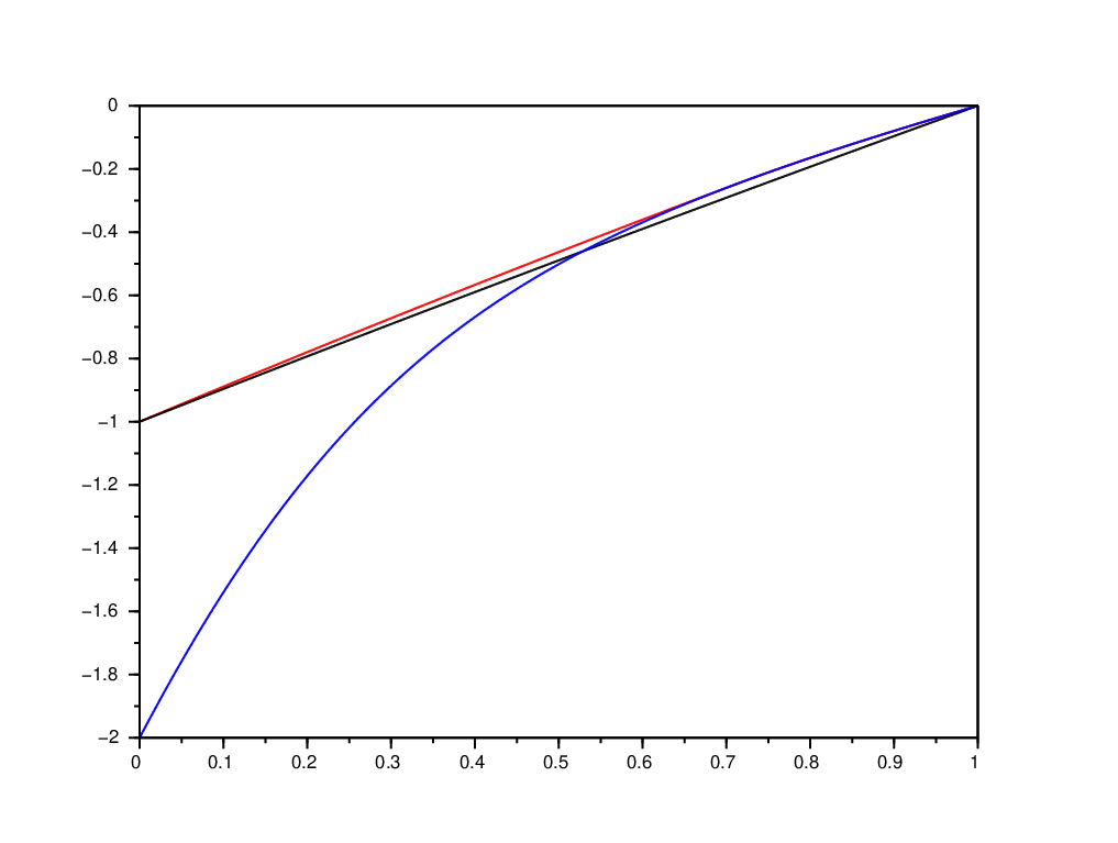
Figure 2. Illustration of Example 4.3 with m=2m=2, p0=.62p_{0}=.62, β=3.22\beta=3.22, λ=.99\lambda=.99 and V00=.99V_{00}=.99 (blue curve: TT; black curve: τν\tau_{\nu}; red curve: τ\tau). qc=q~c=∞q_{c}=\widetilde{q}_{c}=\infty. One second order phase transition at some q0∈(0,1)q_{0}\in(0,1) and one first order phase transition at some q0′∈(1,∞)q^{\prime}_{0}\in(1,\infty). τπ∗​μ=τ>max⁡(τν,T)\tau_{\pi_{*}\mu}=\tau>\max(\tau_{\nu},T) over [0,q0)[0,q_{0}), τπ∗​μ=T=τμ\tau_{\pi_{*}\mu}=T=\tau_{\mu} over [q0′,q0][q^{\prime}_{0},q_{0}], and τπ∗​μ=τν\tau_{\pi_{*}\mu}=\tau_{\nu} over [q0,∞)[q_{0},\infty).
Example 4.4.

This example exhibits two phase transitions over [0,1][0,1] and no first order phase transition over (1,qc)(1,q_{c}), with qc<∞q_{c}<\infty and τπ∗​μ=τμ\tau_{\pi_{*}\mu}=\tau_{\mu} over (1,∞)(1,\infty). Take m=2m=2, p0∈(0,1)p_{0}\in(0,1), and N0N_{0} and N1N_{1} two random integers taking values in {0,1,2}\{0,1,2\} and with positive expectation. Then for 0≤i,j≤10\leq i,j\leq 1 define Vi,j=(𝔼(Ni))−1𝟏{j≤Ni−1}V_{i,j}=({\mathbb{E}}(N_{i}))^{-1}\mathbf{1}_{\{j\leq N_{i}-1\}}. This yields Ti​(q)=(q−1)​log⁡𝔼⁡(Ni)T_{i}(q)=(q-1)\log{\mathbb{E}}(N_{i}), hence Ti∗​(Ti′​(s))=−Ti​(0)=Ti′​(1)=log⁡𝔼⁡(Ni)T_{i}^{*}(T_{i}^{\prime}(s))=-T_{i}(0)=T_{i}^{\prime}(1)=\log{\mathbb{E}}(N_{i}) for all s≥0s\geq 0. Also,

T⁡(q)=−log2⁡(p0q​𝔼​(N0)1−q+(1−p0)q​𝔼​(N1)1−q).T(q)=-\log_{2}\left(p_{0}^{q}{\mathbb{E}}(N_{0})^{1-q}+(1-p_{0})^{q}{\mathbb{E}}(N_{1})^{1-q}\right).

We require 𝔼⁡(N0)<1{\mathbb{E}}(N_{0})<1,

(4.1) 𝔼⁡(N0)​𝔼​(N1)>1,\displaystyle{\mathbb{E}}(N_{0}){\mathbb{E}}(N_{1})>1,
(4.2) 𝔼​(N0)p0​𝔼​(N1)1−p0<1,\displaystyle{\mathbb{E}}(N_{0})^{p_{0}}{\mathbb{E}}(N_{1})^{1-p_{0}}<1,
(4.3) (𝔼⁡(N0)p0)p0​(𝔼⁡(N1)1−p0)1−p0>1.\displaystyle\left(\frac{{\mathbb{E}}(N_{0})}{p_{0}}\right)^{p_{0}}\left(\frac{{\mathbb{E}}(N_{1})}{1-p_{0}}\right)^{1-p_{0}}>1.

Properties (4.2) and (4.3) yield τν′​(1)>T′​(1)>0\tau_{\nu}^{\prime}(1)>T^{\prime}(1)>0. Also (4.1) implies 𝔼⁡(N1)+𝔼⁡(N2)>2{\mathbb{E}}(N_{1})+{\mathbb{E}}(N_{2})>2 hence T⁡(0)<−1=τν​(0)T(0)<-1=\tau_{\nu}(0). The graphs of τν\tau_{\nu} and TT cross each other on [0,1][0,1]. Let GG be defined as in the previous example. Property (4.1) yields ∂G∂s​(q,s)<0\frac{\partial G}{\partial s}(q,s)<0 for all s∈[q,1]s\in[q,1] if qq is close enough to 0, hence τ⁡(q)\tau(q) is attained at q=1q=1; τ​(q)=τν​(q)\tau(q)=\tau_{\nu}(q). Moreover, (4.2) implies that ∂G∂s​(q,s)>0\frac{\partial G}{\partial s}(q,s)>0 for all s∈[q,1]s\in[q,1] if qq is close to 11, hence τ⁡(q)\tau(q) is attained at s=qs=q: τ⁡(q)=T⁡(q)\tau(q)=T(q). Then our study of τ\tau in Section 6 implies that on a non trivial interval we have τ⁡(q)>max⁡(τν​(q),T⁡(q))\tau(q)>\max(\tau_{\nu}(q),T(q)), i.e. τ\tau is given by a third analytic expression.

It is also possible to choose the parameters so that T′​(1)<−log2⁡(p0)=τν′​(+∞)T^{\prime}(1)<-\log_{2}(p_{0})=\tau_{\nu}^{\prime}(+\infty) and p0>𝔼⁡(N0)p_{0}>{\mathbb{E}}(N_{0}), hence τν>T\tau_{\nu}>T over (1,∞)(1,\infty) and qc<∞q_{c}<\infty, which implies that τπ∗​μ​(q)=τμ​(q)\tau_{\pi_{*}\mu}(q)=\tau_{\mu}(q) over [1,∞)[1,\infty). A concrete choice is p0=.8p_{0}=.8, 𝔼⁡(N0)=.6{\mathbb{E}}(N_{0})=.6 and 𝔼⁡(N1)=1.8{\mathbb{E}}(N_{1})=1.8.

Refer to caption
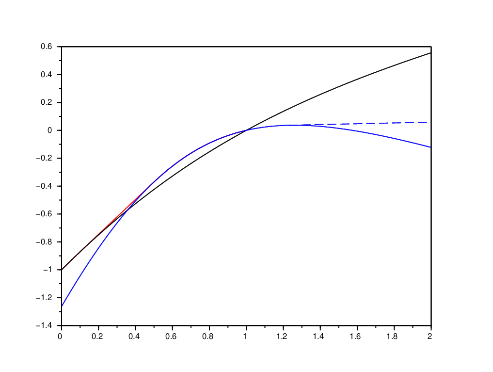
Figure 3. Illustration of Example 4.4 with p0=.8p_{0}=.8, 𝔼⁡(N0)=.6{\mathbb{E}}(N_{0})=.6 and 𝔼⁡(N1)=1.8{\mathbb{E}}(N_{1})=1.8 (blue curve: TT; dashed blue curve: τμ\tau_{\mu}; black curve: τν\tau_{\nu}; red curve: τ\tau). qc=q~c≃1.229<∞q_{c}=\widetilde{q}_{c}\simeq 1.229<\infty. Second order phase transition at some q0<q0′q_{0}<q^{\prime}_{0} in (0,1)(0,1), no first order phase transition over (1,qc)(1,q_{c}), and one second order phase transition at qcq_{c}. τπ∗​μ=τν\tau_{\pi_{*}\mu}=\tau_{\nu} over [0,q0][0,q_{0}], τπ∗​μ=τ>max⁡(τν,T)\tau_{\pi_{*}\mu}=\tau>\max(\tau_{\nu},T) over (q0,q0′)(q_{0},q^{\prime}_{0}), τπ∗​μ=T=τμ\tau_{\pi_{*}\mu}=T=\tau_{\mu} over [q0′,qc][q^{\prime}_{0},q_{c}], and τπ∗​μ​(q)=τμ​(q)=T′​(qc)​q\tau_{\pi_{*}\mu}(q)=\tau_{\mu}(q)=T^{\prime}(q_{c})q over [qc,∞)[q_{c},\infty).
Example 4.5 (Previous example continued).
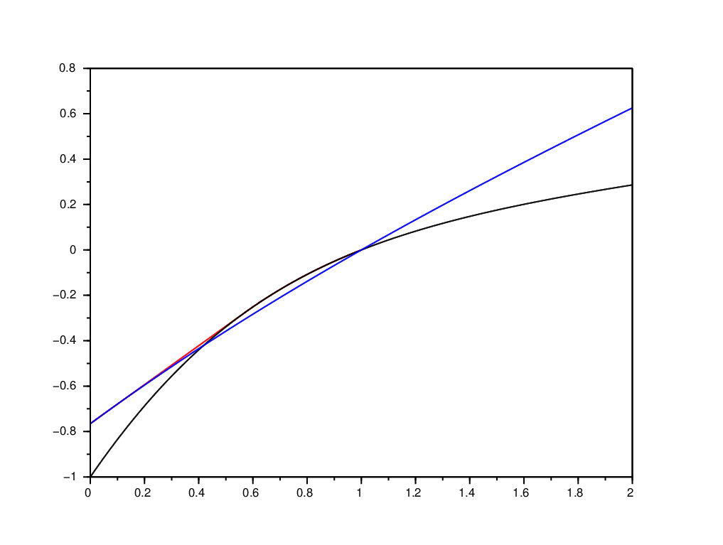
We can use the same model as in Example 4.4 to get other different behaviors. See Figures 4 to 6.

Refer to caption
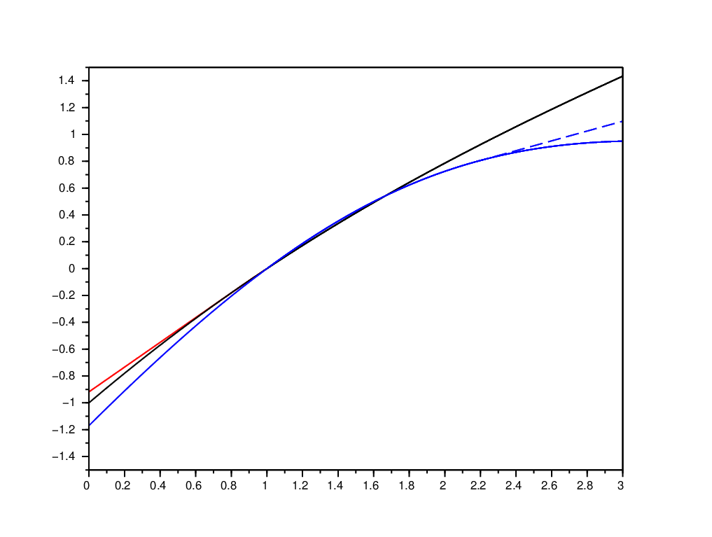
Figure 4. Same model as in Example 4.4 with p0=.1p_{0}=.1, 𝔼⁡(N0)=.4{\mathbb{E}}(N_{0})=.4 and 𝔼⁡(N1)=1.3{\mathbb{E}}(N_{1})=1.3 (blue curve: TT; black curve: τν\tau_{\nu}; red curve: τ\tau). qc=q~c=∞q_{c}=\widetilde{q}_{c}=\infty. Second order phase transitions at some q0<q0′q_{0}<q^{\prime}_{0} in (0,1)(0,1), no first order phase transition over (1,∞)(1,\infty). τπ∗​μ=T=τμ\tau_{\pi_{*}\mu}=T=\tau_{\mu} over [0,q0][0,q_{0}], τπ∗​μ=τ>max⁡(τν,T)\tau_{\pi_{*}\mu}=\tau>\max(\tau_{\nu},T) over (q0,q0′)(q_{0},q^{\prime}_{0}), and τπ∗​μ=τν\tau_{\pi_{*}\mu}=\tau_{\nu} over [q0′,∞)[q^{\prime}_{0},\infty).
Refer to caption
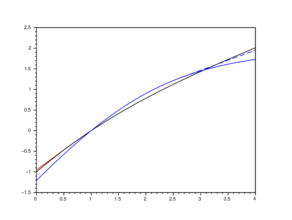
Figure 5. Same model as in Example 4.4 with p0=.3p_{0}=.3, 𝔼⁡(N0)=.25{\mathbb{E}}(N_{0})=.25 and 𝔼⁡(N1)=2{\mathbb{E}}(N_{1})=2 (blue curve: TT; dashed blue curve: τμ\tau_{\mu}; black curve: τν\tau_{\nu}; red curve: τ\tau). qc=q~c≃2.176<∞q_{c}=\widetilde{q}_{c}\simeq 2.176<\infty. One second order phase transition at some q0∈(0,1)q_{0}\in(0,1). One first order phase transition at some q0′∈(1,qc)q^{\prime}_{0}\in(1,q_{c}), and one second order phase transition at qcq_{c}. τπ∗​μ=τ>max⁡(τν,T)\tau_{\pi_{*}\mu}=\tau>\max(\tau_{\nu},T) over [0,q0)[0,q_{0}) (in particular −τ⁡(0)=dimHπ⁡(K)<min⁡(−τν​(0),−T⁡(0))-\tau(0)=\dim_{H}\pi(K)<\min(-\tau_{\nu}(0),-T(0))), τπ∗​μ=τν\tau_{\pi_{*}\mu}=\tau_{\nu} over [q0,q0′][q_{0},q^{\prime}_{0}] and τπ∗​μ=T=τμ\tau_{\pi_{*}\mu}=T=\tau_{\mu} over [q0,qc][q_{0},q_{c}], and τπ∗​μ​(q)=τμ​(q)=T′​(qc)​q\tau_{\pi_{*}\mu}(q)=\tau_{\mu}(q)=T^{\prime}(q_{c})q over [qc,∞)[q_{c},\infty).
Refer to caption
Figure 6. Same model as in Example 4.4 with p0=.3p_{0}=.3, 𝔼⁡(N0)=.3{\mathbb{E}}(N_{0})=.3 and 𝔼⁡(N1)=2{\mathbb{E}}(N_{1})=2 (blue curve: TT; dashed blue curve: τμ\tau_{\mu}; black curve: τν\tau_{\nu}; red curve: τ\tau). qc≃2.665<∞q_{c}\simeq 2.665<\infty and q~c≃3.059\widetilde{q}_{c}\simeq 3.059. One second order phase transition at some q0∈(0,1)q_{0}\in(0,1). No first order phase transition over [1,q~c)[1,\widetilde{q}_{c}). τπ∗​μ=τ>max⁡(τν,T)\tau_{\pi_{*}\mu}=\tau>\max(\tau_{\nu},T) over [0,q0)[0,q_{0}) (in particular −τ⁡(0)=dimHπ⁡(K)<min⁡(−τν​(0),−T⁡(0))-\tau(0)=\dim_{H}\pi(K)<\min(-\tau_{\nu}(0),-T(0))) and τπ∗​μ=τν\tau_{\pi_{*}\mu}=\tau_{\nu} over [q0,q~c][q_{0},\widetilde{q}_{c}].

5. Proofs of Theorem 3.1, Theorem 3.2, and Corollary 3.4

We first introduce the following new notations and definitions.

For each u∈Σ∗u\in\Sigma_{*}, we have

(5.1) π∗​μ​([u])=∑v∈Σ|u|μ⁡([u,v])=∑v∈Σ|u|Q⁡(u,v)​Y​(u,v)=ν⁡(u)​X​(u),\pi_{*}\mu([u])=\sum_{v\in\Sigma_{|u|}}\mu([u,v])=\sum_{v\in\Sigma_{|u|}}Q(u,v)Y(u,v)=\nu(u)X(u),

where

(5.2) X(u)=∑v∈Σ|u|Y(u,v)∏j=1|u|Vuj,vj(u|j−1,v|j−1).X(u)=\sum_{v\in\Sigma_{|u|}}Y(u,v)\prod_{j=1}^{|u|}V_{u_{j},v_{j}}(u_{|j-1},v_{|j-1}).

Define also

X~(u)=∑v∈Σ|u|∏j=1|u|Vuj,vj(u|j−1,v|j−1),\widetilde{X}(u)=\sum_{v\in\Sigma_{|u|}}\prod_{j=1}^{|u|}V_{u_{j},v_{j}}(u_{|j-1},v_{|j-1}),

and for all x∈Σx\in\Sigma and n≥0n\geq 0, set

Xn(x)=X(x|n)andX~n(x)=X~(x|n).X_{n}(x)=X(x_{|n})\quad\text{and}\quad\widetilde{X}_{n}(x)=\widetilde{X}(x_{|n}).

Now, let us start by presenting three results that will be used in this section. They will be proved in Section 9, where they appear as Proposition 9.8, Corollary 9.9, and Proposition 9.13 respectively.

Proposition 5.1.

Let q>1q>1 such that T⁡(q)>0T(q)>0. Let η\eta be the Bernoulli product measure on Σ\Sigma generated by a probability vector (p0′,…,pm−1′)(p_{0}^{\prime},\ldots,p_{m-1}^{\prime}). Set A:=max⁡{1,∑i=0m−1pi′​m−Ti​(q)}A:=\max\{1,\sum_{i=0}^{m-1}p_{i}^{\prime}m^{-T_{i}(q)}\}. Then there exists a polynomial fqf_{q} depending on WW and qq such that

(5.3) An≤𝔼ℙ⊗η​(Xnq)≤fq​(n)​An,∀n∈ℕ.A^{n}\leq\mathbb{E}_{\mathbb{P}\otimes\eta}(X_{n}^{q})\leq f_{q}(n)A^{n},\quad\forall n\in{\mathbb{N}}.

Furthermore, when q∈(1,2]q\in(1,2], fq​(n)f_{q}(n) can be taken as a constant.

Corollary 5.2.

Let q>1q>1 such that T⁡(q)>0T(q)>0. Then there exists a polynomial fqf_{q} depending on WW and qq such that

(5.4) m−n​min⁡{τν​(q),T⁡(q)}≤𝔼⁡(∑u∈Σnπ∗​μ​([u])q)≤fq​(n)​m−n​min⁡{τν​(q),T⁡(q)}m^{-n\min\{\tau_{\nu}(q),T(q)\}}\leq\mathbb{E}\Big(\sum_{u\in\Sigma_{n}}\pi_{*}\mu([u])^{q}\Big)\leq f_{q}(n)m^{-n\min\{\tau_{\nu}(q),T(q)\}}

for all n∈ℕn\in{\mathbb{N}}.

Proposition 5.3.

Let η\eta be the Bernoulli product measure on Σ\Sigma generated by a probability vector (p0′,…,pm−1′)(p_{0}^{\prime},\ldots,p_{m-1}^{\prime}). Assume that T⁡(q)>0T(q)>0 and ∑i=0m−1pi′​m−Ti​(q)<1\sum_{i=0}^{m-1}p_{i}^{\prime}m^{-T_{i}(q)}<1 for some q∈(1,2]q\in(1,2], and that there exists c∈(0,1)c\in(0,1) such that the following two conditions are satisfied:

  • (i)

    ℙ⁡(sup0≤j≤m−1Vi,j>c)=1\mathbb{P}(\sup_{0\leq j\leq m-1}V_{i,j}>c)=1 for all 0≤i≤m−10\leq i\leq m-1;

  • (ii)

    𝔼⁡(#⁡{j:Vi,j>c})>1{\mathbb{E}}(\#\{j:V_{i,j}>c\})>1 for all 0≤i≤m−10\leq i\leq m-1.

Then there exists b>0b>0 such that

supn≥1𝔼ℙ⊗η​(Xn−b)<∞.\sup_{n\geq 1}{\mathbb{E}}_{\mathbb{P}\otimes\eta}(X_{n}^{-b})<\infty.

5.1. Proof of Theorem 3.1

Proof of Theorem 3.1(1).

(i) Since (Σ,d)(\Sigma,d) satisfies the Besicovitch covering property, we have almost surely π∗​μω​(d​x)=f⁡(ω,x)​ν​(d​x)+ρω​(d​x)\pi_{*}\mu_{\omega}(\mathrm{d}x)=f(\omega,x)\,\nu(\mathrm{d}x)+\rho_{\omega}(\mathrm{d}x), where ρω\rho_{\omega} is a Borel measure singular with respect to ν\nu and

(5.5) f⁡(ω,x)=limn→∞(Xn​(ω,x)=π∗μω([x|n])ν(x|n)),f(\omega,x)=\lim_{n\to\infty}\left(X_{n}(\omega,x)=\frac{\pi_{*}\mu_{\omega}([x_{|n}])}{\nu(x_{|n})}\right),

ν\nu-almost everywhere. Thus, if 𝔼ℙ⊗ν​(f)=𝔼⁡(‖π∗​μ‖)=1\mathbb{E}_{\mathbb{P}\otimes\nu}(f)=\mathbb{E}(\|\pi_{*}\mu\|)=1, we have ρω=0\rho_{\omega}=0 almost surely, i.e. π∗​μ\pi_{*}\mu is almost surely absolutely continuous with respect to ν\nu.

We know by the construction of μ\mu that for all n≥1n\geq 1 we have 𝔼ℙ⊗ν​(Xn)=𝔼⁡(‖μn‖)=1\mathbb{E}_{\mathbb{P}\otimes\nu}(X_{n})={\mathbb{E}}(\|\mu_{n}\|)=1. This implies that for all λ∈(0,1)\lambda\in(0,1) the sequence (Xnλ)n≥1(X_{n}^{\lambda})_{n\geq 1} is uniformly integrable with respect to ℙ⊗ν\mathbb{P}\otimes\nu, hence by (5.5) we have limn→∞𝔼ℙ⊗ν​(Xnλ)=𝔼ℙ⊗ν​(fλ)\lim_{n\to\infty}\mathbb{E}_{\mathbb{P}\otimes\nu}(X_{n}^{\lambda})=\mathbb{E}_{\mathbb{P}\otimes\nu}(f^{\lambda}).

Next we claim that under ℙ⊗ν\mathbb{P}\otimes\nu, XnX_{n} converges in law to a random variable X~\widetilde{X}. We postpone its proof to the next paragraph. Since for any given λ∈(0,1)\lambda\in(0,1) the sequence (Xnλ)n≥1(X_{n}^{\lambda})_{n\geq 1} is uniformly integrable, we have limn→∞𝔼ℙ⊗ν​(Xnλ)=𝔼ℙ⊗ν​(X~λ)\lim_{n\to\infty}\mathbb{E}_{\mathbb{P}\otimes\nu}(X_{n}^{\lambda})={\mathbb{E}}_{\mathbb{P}\otimes\nu}(\widetilde{X}^{\lambda}). Hence 𝔼ℙ⊗ν​(fλ)=𝔼ℙ⊗ν​(X~λ)\mathbb{E}_{\mathbb{P}\otimes\nu}(f^{\lambda})={\mathbb{E}}_{\mathbb{P}\otimes\nu}(\widetilde{X}^{\lambda}) for all λ∈(0,1)\lambda\in(0,1). Furthermore, if 𝔼ℙ⊗ν​(X~)=1{\mathbb{E}}_{\mathbb{P}\otimes\nu}(\widetilde{X})=1, letting λ\lambda tend to 1 we get 𝔼ℙ⊗ν​(f)=1\mathbb{E}_{\mathbb{P}\otimes\nu}(f)=1.

We now prove that XnX_{n} converges in law to a random variable X~\widetilde{X} such that 𝔼ℙ⊗ν​(X~)=1{\mathbb{E}}_{\mathbb{P}\otimes\nu}(\widetilde{X})=1.

By the definition of Xn​(x)X_{n}(x), for any t>0t>0 we have

𝔼ℙ⊗ν(e−t​Xn)=𝔼ℙ⊗ν(∏v∈ΣnϕY(t∏j=1nVxj,vj(x|j−1,v|j−1)),\mathbb{E}_{\mathbb{P}\otimes\nu}(e^{-tX_{n}})=\mathbb{E}_{\mathbb{P}\otimes\nu}\Big(\prod_{v\in\Sigma_{n}}\phi_{Y}\Big(t\prod_{j=1}^{n}V_{x_{j},v_{j}}(x_{|j-1},v_{|j-1})\Big),

where ϕY\phi_{Y} stands for the Laplace transform of YY, i.e. ϕY​(t)=𝔼⁡(e−t​Y)\phi_{Y}(t)=\mathbb{E}(e^{-tY}).

Let us show that

Mn(x):=maxv∈Σn∏j=1nVxj,vj(x|j−1,v|j−1)M_{n}(x):=\max_{v\in\Sigma_{n}}\prod_{j=1}^{n}V_{x_{j},v_{j}}(x_{|j-1},v_{|j-1})

converges in law to 0 under ℙ⊗ν\mathbb{P}\otimes\nu, as nn tends to ∞\infty. For x∈Σx\in\Sigma, let ℚx\mathbb{Q}_{x} be the probability measure on

(Ω×Σ,σ(Vxn(x|n−1,v):n≥1,v∈Σn−1)⊗ℬ(Σ))(\Omega\times\Sigma,\sigma(V_{x_{n}}(x_{|n-1},v):n\geq 1,\,v\in\Sigma_{n-1})\otimes\mathcal{B}(\Sigma))

whose restriction to

σ(Vxj(x|n−1,v):1≤j≤n,v∈Σj−1)⊗σ([v]:v∈Σn)\sigma(V_{x_{j}}(x_{|n-1},v):1\leq j\leq n,\,v\in\Sigma_{j-1})\otimes\sigma([v]:v\in\Sigma_{n})

is determined by

ℚx,n(A×[v])=𝔼(𝟏A(ω)∏j=1nVxj,vj(x|j−1,v|j−1))\mathbb{Q}_{x,n}(A\times[v])=\mathbb{E}\big(\mathbf{1}_{A}(\omega)\prod_{j=1}^{n}V_{x_{j},v_{j}}(x_{|j-1},v_{|j-1})\big)

for A∈σ(Vxj(v):1≤j≤n,v∈Σj−1)A\in\sigma(V_{x_{j}}(v):1\leq j\leq n,\,v\in\Sigma_{j-1}) and v∈Σnv\in\Sigma_{n}. This yields a new skew product measure ρ⁡(d​ω,d​x,d​y)=ν⁡(d​x)​ℚx​(d​ω,d​y)\rho(\mathrm{d}\omega,\mathrm{d}x,\mathrm{d}y)=\nu(\mathrm{d}x)\mathbb{Q}_{x}(\mathrm{d}\omega,\mathrm{d}y) on Ω×Σ2\Omega\times\Sigma^{2}. A direct computation shows that the random variables (ω,x,y)↦Vxj,yj(x|j−1,y|j−1)(\omega,x,y)\mapsto V_{x_{j},y_{j}}(x_{|j-1},y_{|j-1}) are i.i.d. with respect to ρ\rho, and their logarithms are of expectation

∑i=0m−1pi∑j=0m−1𝔼(Vi,jlogVi,j)=−log(m)∑i=0m−1piTi′(1−)<0.\sum_{i=0}^{m-1}p_{i}\sum_{j=0}^{m-1}{\mathbb{E}}(V_{i,j}\log V_{i,j})=-\log(m)\sum_{i=0}^{m-1}p_{i}T_{i}^{\prime}(1-)<0.

It follows from the strong law of large numbers that for ρ\rho-almost every (ω,x,y)(\omega,x,y) one has

limn→∞∏j=1nVxj,yj(x|j−1,y|j−1)=0.\lim_{n\to\infty}\prod_{j=1}^{n}V_{x_{j},y_{j}}(x_{|j-1},y_{|j-1})=0.

Now fix ϵ>0\epsilon>0. We have

ℙ⊗ν⁡(Mn​(x)≥ϵ)\displaystyle\mathbb{P}\otimes\nu(M_{n}(x)\geq\epsilon) ≤\displaystyle\leq 𝔼ℙ⊗ν(∑v∈Σn𝟏{∏j=1nVxj,vj(x|j−1,v|j−1)≥ϵ})\displaystyle{\mathbb{E}}_{\mathbb{P}\otimes\nu}\Big(\sum_{v\in\Sigma_{n}}\mathbf{1}_{\{\prod_{j=1}^{n}V_{x_{j},v_{j}}(x_{|j-1},v_{|j-1})\geq\epsilon\}}\Big)
≤\displaystyle\leq 𝔼ℙ⊗ν(∑v∈Σnϵ−1𝟏{∏j=1nVxj,vj(x|j−1,v|j−1)≥ϵ}∏j=1nVxj,vj(x|j−1,v|j−1))\displaystyle{\mathbb{E}}_{\mathbb{P}\otimes\nu}\Big(\sum_{v\in\Sigma_{n}}\epsilon^{-1}\mathbf{1}_{\{\prod_{j=1}^{n}V_{x_{j},v_{j}}(x_{|j-1},v_{|j-1})\geq\epsilon\}}\prod_{j=1}^{n}V_{x_{j},v_{j}}(x_{|j-1},v_{|j-1})\Big)
=\displaystyle= ϵ−1ρ({∏j=1nVxj,yj(x|j−1,y|j−1)≥ϵ}),\displaystyle\epsilon^{-1}\rho\Big(\Big\{\prod_{j=1}^{n}V_{x_{j},y_{j}}(x_{|j-1},y_{|j-1})\geq\epsilon\Big\}\Big),

and the right hand side converges to 0.

Consequently, since 𝔼⁡(Y)=1\mathbb{E}(Y)=1, we have ϕY​(u)=e−u+o⁡(u)\phi_{Y}(u)=e^{-u+o(u)} near 0+0+, so for each t>0t>0 we can write

(5.6) 𝔼ℙ⊗ν​(e−t​Xn)\displaystyle\mathbb{E}_{\mathbb{P}\otimes\nu}(e^{-tX_{n}}) =\displaystyle= 𝔼ℙ⊗ν(𝟏{Mn(x)<ϵ}e−t​X~n​(1+O⁡(ϵ)))+𝔼ℙ⊗ν(𝟏{Mn(x)≥ϵ}e−t​Xn)\displaystyle\mathbb{E}_{\mathbb{P}\otimes\nu}\Big(\mathbf{1}_{\{M_{n}(x)<\epsilon\}}e^{-t\widetilde{X}_{n}(1+O(\epsilon))}\Big)+\mathbb{E}_{\mathbb{P}\otimes\nu}\Big(\mathbf{1}_{\{M_{n}(x)\geq\epsilon\}}e^{-tX_{n}}\Big)
=\displaystyle= 𝔼ℙ⊗ν​(e−t​X~n​(1+O⁡(ϵ)))+Rn,\displaystyle\mathbb{E}_{\mathbb{P}\otimes\nu}\Big(e^{-t\widetilde{X}_{n}(1+O(\epsilon))}\Big)+R_{n},

where |Rn|≤2​ℙ⊗ν⁡(Mn​(x)≥ϵ)|R_{n}|\leq 2\mathbb{P}\otimes\nu(M_{n}(x)\geq\epsilon) and X~n​(1+O⁡(ϵ))≥0\widetilde{X}_{n}(1+O(\epsilon))\geq 0. On the other hand, the information gathered in Appendix B applied with η=ν\eta=\nu and Ui=ViU_{i}=V_{i} shows that (X~n​(x,⋅))n≥1(\widetilde{X}_{n}(x,\cdot))_{n\geq 1} is a Mandelbrot martingale in the random environment defined by ν\nu, and X~n\widetilde{X}_{n} converges ℙ⊗ν\mathbb{P}\otimes\nu-almost surely to a limit X~\widetilde{X}. We then deduce from the bounded convergence theorem and the fact that ℙ⊗ν⁡(Mn​(x)≥ϵ)\mathbb{P}\otimes\nu(M_{n}(x)\geq\epsilon) tends to 0 as n→∞n\to\infty that 𝔼ℙ⊗ν​(e−t​Xn){\mathbb{E}}_{\mathbb{P}\otimes\nu}(e^{-tX_{n}}) converges to 𝔼ℙ⊗ν​(e−t​X~){\mathbb{E}}_{\mathbb{P}\otimes\nu}(e^{-t\widetilde{X}}). Moreover, the condition dim(μ)−dim(ν)=∑i=0m−1pi​Ti′​(1−)>0\dim(\mu)-\dim(\nu)=\sum_{i=0}^{m-1}p_{i}T_{i}^{\prime}(1-)>0 is sufficient for (X~n)n≥1(\widetilde{X}_{n})_{n\geq 1} to be uniformly integrable (Theorem B.1), hence 𝔼ℙ⊗ν​(X~)=1{\mathbb{E}}_{\mathbb{P}\otimes\nu}(\widetilde{X})=1.

(ii) Since T′​(1−)>0T^{\prime}(1-)>0, the assumption that TT is finite on a neighborhood of 11 implies that T⁡(s)>0T(s)>0, hence 𝔼⁡(Ys)<∞{\mathbb{E}}(Y^{s})<\infty on a right neighborhood of 11 (see [37] or [11]). Moreover, the assumption dim(μ)>dim(ν)\dim(\mu)>\dim(\nu) is equivalent to ∑i=0m−1pi​Ti′​(1)>0\sum_{i=0}^{m-1}p_{i}T_{i}^{\prime}(1)>0, hence we have ∑i=0m−1pi​m−Ti​(s)<1\sum_{i=0}^{m-1}p_{i}m^{-T_{i}(s)}<1 on a right neighborhood of 11. Also, if s∈(1,2]s\in(1,2] and both 𝔼⁡(Ys)<∞{\mathbb{E}}(Y^{s})<\infty and ∑i=0m−1pi​m−Ti​(s)<1\sum_{i=0}^{m-1}p_{i}m^{-T_{i}(s)}<1, then supn≥1𝔼ℙ⊗ν​(Xn​(x)s)<∞\sup_{n\geq 1}\mathbb{E}_{\mathbb{P}\otimes\nu}(X_{n}(x)^{s})<\infty by Proposition 5.1. For any such s>1s>1, using (5.1) we get

∫Σ(π∗μ([x|n])ν([x|n]))s−1π∗μ(dx)=∑u∈Σn𝟏{ν([u])>0}(π∗​μ​([u])ν⁡([u]))s−1π∗μ([u])=∑u∈Σnν([u])X(u)s.\displaystyle\int_{\Sigma}\Big(\frac{\pi_{*}\mu([x_{|n}])}{\nu([x_{|n}])}\Big)^{s-1}\,\pi_{*}\mu(\mathrm{d}x)=\sum_{u\in\Sigma_{n}}\mathbf{1}_{\{\nu([u])>0\}}\Big(\frac{\pi_{*}\mu([u])}{\nu([u])}\Big)^{s-1}\pi_{*}\mu([u])=\sum_{u\in\Sigma_{n}}\nu([u])X(u)^{s}.

Thus

supn≥1𝔼⁡(∫Σ(π∗μ([x|n])ν([x|n]))s−1​π∗​μ​(𝑑x))=supn≥1𝔼ℙ⊗ν​(Xn​(x)s)<∞.\displaystyle\sup_{n\geq 1}{\mathbb{E}}\left(\int_{\Sigma}\Big(\frac{\pi_{*}\mu([x_{|n}])}{\nu([x_{|n}])}\Big)^{s-1}\,\pi_{*}\mu(\mathrm{d}x)\right)=\sup_{n\geq 1}\mathbb{E}_{\mathbb{P}\otimes\nu}(X_{n}(x)^{s})<\infty.

Consequently, by the Fatou lemma,

𝔼⁡(lim infn→∞∫Σ(π∗μ([x|n])ν([x|n]))s−1​π∗​μ​(𝑑x))\displaystyle{\mathbb{E}}\left(\liminf_{n\to\infty}\int_{\Sigma}\Big(\frac{\pi_{*}\mu([x_{|n}])}{\nu([x_{|n}])}\Big)^{s-1}\,\pi_{*}\mu(\mathrm{d}x)\right) ≤\displaystyle\leq lim infn→∞𝔼⁡(∫Σ(π∗μ([x|n])ν([x|n]))s−1​π∗​μ​(𝑑x))\displaystyle\liminf_{n\to\infty}{\mathbb{E}}\left(\int_{\Sigma}\Big(\frac{\pi_{*}\mu([x_{|n}])}{\nu([x_{|n}])}\Big)^{s-1}\,\pi_{*}\mu(\mathrm{d}x)\right)
<\displaystyle< ∞,\displaystyle\infty,

from which we get

lim infn→∞∫Σ(π∗μ([x|n])ν([x|n]))s−1​π∗​μ​(𝑑x)<∞a.s.\liminf_{n\to\infty}\int_{\Sigma}\Big(\frac{\pi_{*}\mu([x_{|n}])}{\nu([x_{|n}])}\Big)^{s-1}\,\pi_{*}\mu(\mathrm{d}x)<\infty\quad\text{a.s.}

Due to [46, Theorem 2.12(3)], this implies both the absolute continuity of π∗​μ\pi_{*}\mu with respect to ν\nu and the desired result about the density of π∗​μ\pi_{*}\mu with respect to ν\nu.

(iii) At first notice that our assumption implies that the support of π∗​μ\pi_{*}\mu equals that of ν\nu almost surely. In particular, X⁡(u)>0X(u)>0 for all uu such that ν⁡(u)>0\nu(u)>0. Thus, for any s>1s>1 we have almost surely

∑u∈Σn𝟏{π∗μ([u])>0}(ν⁡([u])π∗​μ​([u]))s−1ν([u])=∑u∈Σn𝟏{ν([u])>0}ν([u])X(u)1−s\sum_{u\in\Sigma_{n}}\mathbf{1}_{\{\pi_{*}\mu([u])>0\}}\Big(\frac{\nu([u])}{\pi_{*}\mu([u])}\Big)^{s-1}\nu([u])=\sum_{u\in\Sigma_{n}}\mathbf{1}_{\{\nu([u])>0\}}\nu([u])X(u)^{1-s}

and

𝔼(∑u∈Σn𝟏{π∗μ([u])>0}(ν⁡([u])π∗​μ​([u]))s−1ν([u]))=𝔼ℙ⊗ν(Xn(x)1−s).\displaystyle{\mathbb{E}}\Big(\sum_{u\in\Sigma_{n}}\mathbf{1}_{\{\pi_{*}\mu([u])>0\}}\Big(\frac{\nu([u])}{\pi_{*}\mu([u])}\Big)^{s-1}\nu([u])\Big)=\mathbb{E}_{\mathbb{P}\otimes\nu}(X_{n}(x)^{1-s}).

Due to our assumption on the random vectors ViV_{i} and the fact that for qq close enough to 1 we have ∑i=0m−1pi​m−Ti​(q)<1\sum_{i=0}^{m-1}p_{i}m^{-T_{i}(q)}<1, Proposition 5.3 yields supn≥1𝔼ℙ⊗ν​(Xn​(x)1−s)<∞\sup_{n\geq 1}\mathbb{E}_{\mathbb{P}\otimes\nu}(X_{n}(x)^{1-s})<\infty if ss is close enough to 1. Similarly to (ii), this implies

lim infn→∞∫Σ(ν([x|n])π∗μ([x|n]))s−1​ν​(𝑑x)<∞a.s.\liminf_{n\to\infty}\int_{\Sigma}\Big(\frac{\nu([x_{|n}])}{\pi_{*}\mu([x_{|n}])}\Big)^{s-1}\,\nu(\mathrm{d}x)<\infty\quad\text{a.s.}

hence both the absolute continuity of ν\nu with respect to π∗​μ\pi_{*}\mu and the desired result about the density of ν\nu with respect to π∗​μ\pi_{*}\mu. ∎

Proof of Theorem 3.1(2).

If dim(μ)<dim(ν)\dim(\mu)<\dim(\nu), there is nothing to prove since dim¯P​(π∗​μ)≤dim(μ)\overline{\dim}_{P}(\pi_{*}\mu)\leq\dim(\mu).

Suppose now that dim(μ)=T′​(1)=dim(ν)\dim(\mu)=T^{\prime}(1)=\dim(\nu). This time, under ℙ⊗ν\mathbb{P}\otimes\nu, the martingale X~n​(ω,x)\widetilde{X}_{n}(\omega,x) converges to 0 almost surely since ∑i=0m−1pi​Ti′​(1−)=0\sum_{i=0}^{m-1}p_{i}T_{i}^{\prime}(1-)=0 (see Theorem B.1 again). This implies that Mn(x)=maxv∈Σn∏j=1nVxj,vj(x|j−1,v|j−1)M_{n}(x)=\max_{v\in\Sigma_{n}}\prod_{j=1}^{n}V_{x_{j},v_{j}}(x_{|j-1},v_{|j-1}) converge to 0 almost surely under ℙ⊗ν\mathbb{P}\otimes\nu. Using (5.6) this time yields the convergence in law to 0 for XnX_{n}, and 𝔼ℙ⊗ν​(fλ)=0{\mathbb{E}}_{\mathbb{P}\otimes\nu}(f^{\lambda})=0 for all λ∈(0,1)\lambda\in(0,1). Consequently, f=0f=0 with ℙ⊗ν\mathbb{P}\otimes\nu probability 1, which is equivalent to the fact that π∗​μ\pi_{*}\mu and ν\nu are almost surely mutually singular. ∎

5.2. Proof of Theorem 3.2(1)

When dim(μ)>dim(ν)\dim(\mu)>\dim(\nu), since by Theorem 3.1(1)(i) π∗​μ\pi_{*}\mu is absolutely continuous with respect to ν\nu, we already know that if μ≠0\mu\neq 0, we have dim(π∗​μ)=dim(ν)\dim(\pi_{*}\mu)=\dim(\nu). However, under the assumption that TT is finite in a neighborhood of 1, we give an alternative proof which works regardless of the respective positions of dim(μ)\dim(\mu) and dim(ν)\dim(\nu), and independently of absolute continuity considerations.

We will use Corollary 5.2 and the following elementary lemma.

Lemma 5.4.

Let ρ\rho be a positive and finite Borel measure on Σ\Sigma. Let D≥0D\geq 0. If for all ϵ>0\epsilon>0 there exists q>1q>1 such that ∑n≥1mn​(q−1)​(D−ϵ)​∑|u|=nρ​([u])q<∞\sum_{n\geq 1}m^{n(q-1)(D-\epsilon)}\sum_{|u|=n}\rho([u])^{q}<\infty, then dim¯loc​(ρ,x)≥D\underline{\dim}_{\rm loc}(\rho,x)\geq D for ρ\rho-almost every xx. Also, if for all ϵ>0\epsilon>0 there exists q∈(0,1)q\in(0,1) such that ∑n≥1mn​(q−1)​(D+ϵ)​∑|u|=nρ​([u])q<∞\sum_{n\geq 1}m^{n(q-1)(D+\epsilon)}\sum_{|u|=n}\rho([u])^{q}<\infty, then dim¯loc​(ρ,x)≤D\overline{\dim}_{\rm loc}(\rho,x)\leq D for ρ\rho-almost every xx.

Proof.

Fix ϵ>0\epsilon>0. For all q>1q>1 and n≥1n\geq 1, applying Markov’s inequality we have

ρ⁡({x∈Σ:log(ρ([x|n]))−n​log⁡(m)≤D−ϵ})\displaystyle\rho\Big(\Big\{x\in\Sigma:\;\frac{\log(\rho([x_{|n}]))}{-n\log(m)}\leq D-\epsilon\Big\}\Big) =\displaystyle= ρ({x∈Σ:ρ([x|n])q−1≥m−n​(q−1)​(D−ϵ)})\displaystyle\rho\Big(\Big\{x\in\Sigma:\;\rho([x_{|n}])^{q-1}\geq m^{-n(q-1)(D-\epsilon)}\Big\}\Big)
≤\displaystyle\leq mn​(q−1)​(D−ϵ)∫Σρ([x|n])q−1ρ(dx)\displaystyle m^{n(q-1)(D-\epsilon)}\ \int_{\Sigma}\rho([x_{|n}])^{q-1}\,\rho(\mathrm{d}x)
=\displaystyle= mn​(q−1)​(D−ϵ)​∑|u|=nρ​([u])q.\displaystyle m^{n(q-1)(D-\epsilon)}\sum_{|u|=n}\rho([u])^{q}.

Consequently, if ∑n≥1mn​(q−1)​(D−ϵ)​∑|u|=nρ​([u])q<∞\sum_{n\geq 1}m^{n(q-1)(D-\epsilon)}\sum_{|u|=n}\rho([u])^{q}<\infty, by the Borel-Cantelli lemma we get dim¯loc​(ρ,x)≥D−ϵ\underline{\dim}_{\rm loc}(\rho,x)\geq D-\epsilon for ρ\rho-almost every xx.

The upper local dimension of ρ\rho is dealt with similarly. ∎

Recall that dim(ν)=τν′​(1)\dim(\nu)=\tau_{\nu}^{\prime}(1) and that almost surely, conditionally on μ≠0\mu\neq 0, dim(μ)=T′​(1)\dim(\mu)=T^{\prime}(1). We deduce from corollary 5.2 that for q>1q>1 close enough to 1, there exists a polynomial function fqf_{q} such that for all n≥1n\geq 1 we have

𝔼⁡(∑u∈Σnπ∗​μ​([u])q)≤fq​(n)⋅{m−n(q−1)dim(ν)+o(q−1)if ​T′​(1)>τν′​(1)m−n⁡(q−1)​T′​(1)+o⁡(q−1)if ​T′​(1)≤τν′​(1)\displaystyle\mathbb{E}\Big(\sum_{u\in\Sigma_{n}}\pi_{*}\mu([u])^{q}\Big)\leq f_{q}(n)\cdot\begin{cases}m^{-n(q-1)\dim(\nu)+o(q-1)}&\text{if }T^{\prime}(1)>\tau_{\nu}^{\prime}(1)\\ m^{-n(q-1)T^{\prime}(1)+o(q-1)}&\text{if }T^{\prime}(1)\leq\tau_{\nu}^{\prime}(1)\end{cases}

as q→1+q\to 1+. Fix ϵ>0\epsilon>0. Take qq close enough to 11 so that the previous upper bound holds with |o⁡(q−1)|≤ϵ⁡(q−1)/4|o(q-1)|\leq\epsilon(q-1)/4. By Lemma C.1 we conclude that, with probability 1, conditionally on μ≠0\mu\neq 0, for nn large enough we have

mn​(q−1)​(D−ϵ)∑|u|=nπ∗μ([u])q≤m−nϵ(q−1)/2,m^{n(q-1)(D-\epsilon)}\sum_{|u|=n}\pi_{*}\mu([u])^{q}\leq m^{-n\epsilon(q-1)/2},

with D=τν′​(1)D=\tau_{\nu}^{\prime}(1) if T′​(1)>τν′​(1)T^{\prime}(1)>\tau_{\nu}^{\prime}(1), and D=T′​(1)D=T^{\prime}(1) otherwise. Then Lemma 5.4 yields the expected lower bound for dim¯loc​(π∗​μ,x)\underline{\dim}_{\rm loc}(\pi_{*}\mu,x), π∗​μ\pi_{*}\mu-almost everywhere.

To control dim¯loc​(π∗​μ,x)\overline{\dim}_{\rm loc}(\pi_{*}\mu,x), π∗​μ\pi_{*}\mu-almost everywhere, we only need to deal with the case T′​(1)>τν′​(1)T^{\prime}(1)>\tau_{\nu}^{\prime}(1). Indeed, for π∗​μ\pi_{*}\mu-almost every xx, we obviously have dim¯loc​(π∗​μ,x)≤dim(μ)\overline{\dim}_{\rm loc}(\pi_{*}\mu,x)\leq\dim(\mu).

Now assume T′​(1)>τν′​(1)T^{\prime}(1)>\tau_{\nu}^{\prime}(1). Let q∈(0,1)q\in(0,1). We have

𝔼⁡(∑u∈Σnπ∗​μ​([u])q)\displaystyle\mathbb{E}\Big(\sum_{u\in\Sigma_{n}}\pi_{*}\mu([u])^{q}\Big) =\displaystyle= ∑u∈Σnν​([u])q​𝔼​(X​(u)q)\displaystyle\sum_{u\in\Sigma_{n}}\nu([u])^{q}\mathbb{E}(X(u)^{q})
≤\displaystyle\leq ∑u∈Σnν​([u])q​𝔼​(X⁡(u))q=∑u∈Σnν​([u])q=m−n​τν​(q).\displaystyle\sum_{u\in\Sigma_{n}}\nu([u])^{q}\mathbb{E}(X(u))^{q}=\sum_{u\in\Sigma_{n}}\nu([u])^{q}=m^{-n\tau_{\nu}(q)}.

This is enough to conclude that dim¯loc​(π∗​μ,x)≤τν′​(1)\overline{\dim}_{\rm loc}(\pi_{*}\mu,x)\leq\tau_{\nu}^{\prime}(1) for π∗​μ\pi_{*}\mu-almost every xx by using again Lemmas C.1 and 5.4.

Putting together the previous arguments we conclude that with probability 1, conditionally on μ≠0\mu\neq 0, π∗​μ\pi_{*}\mu is exactly dimensional with dim(π∗​μ)=dim(ν)\dim(\pi_{*}\mu)=\dim(\nu) if T′​(1)>τν′​(1)T^{\prime}(1)>\tau_{\nu}^{\prime}(1) and dim(π∗​μ)=dim(μ)\dim(\pi_{*}\mu)=\dim(\mu) if T′​(1)≤τν′​(1)T^{\prime}(1)\leq\tau_{\nu}^{\prime}(1).

5.3. Proof of Theorem 3.2(2): Two approaches to the dimension of the conditional measures

We will give two different approaches to the calculation of the dimension of the conditional measures. The first one will assume that TT is finite in a neighborhood of 11 and adapt the original approach by Peyrière [37] and Liu-Rouault [42] to compute the dimensions of Mandelbrot measures. The second one, more, conceptual, will require no additional assumption, and combine a reduction to the case of Mandelbrot measures in random environment with the percolation approach developed by Kahane [36] to remove the extra hypothesis assumed on the moments of orders greater than 1 in [37, 42] in the case of Mandelbrot measures.

We start with preliminary definitions. When μ≠0\mu\neq 0, for π∗​μω\pi_{*}\mu_{\omega}-almost every xx, there exists a conditional measure μωx\mu^{x}_{\omega} supported on Kx=π−1​({x})∩KK^{x}=\pi^{-1}(\{x\})\cap K, obtained as the weak-star limit, as n→∞n\to\infty, of the measures μω,nx\mu_{\omega,n}^{x} obtained on π−1​({x})\pi^{-1}(\{x\}) by assigning uniformly the mass μω([x|n]×[J])π∗μω([x|n])\frac{\mu_{\omega}([x_{|n}]\times[J])}{\pi_{*}\mu_{\omega}([x_{|n}])} to each cylinder [J][J] of generation nn, so that we have

μω​(d​x,d​y)=π∗​μω​(d​x)​μωx​(d​y).\mu_{\omega}(\mathrm{d}x,\mathrm{d}y)=\pi_{*}\mu_{\omega}(\mathrm{d}x)\mu^{x}_{\omega}(\mathrm{d}y).

To be more specific, for any cylinder [J][J], almost surely, the measurable set

AJ={(ω,x)∈Ω×Σ:limn→∞μω([x|n]×[J])π∗μω([x|n])​ exists}A_{J}=\{(\omega,x)\in\Omega\times\Sigma:\lim_{n\to\infty}\frac{\mu_{\omega}([x_{|n}]\times[J])}{\pi_{*}\mu_{\omega}([x_{|n}])}\text{ exists}\}

is of full ℚ^\widehat{\mathbb{Q}}-probability, where we define ℚ^​(d​ω,d​x)=ℙ⁡(d​ω)​π∗​μω​(d​x)\widehat{\mathbb{Q}}({\rm d}\omega,{\rm d}x)=\mathbb{P}({\rm d}\omega)\pi_{*}\mu_{\omega}(\mathrm{d}x), and for all (ω,x)(\omega,x) in a subset AJ′A^{\prime}_{J} of AJA_{J} of full ℚ^\widehat{\mathbb{Q}}-probability, we have μωx​(J)=limn→∞μω([x|n]×[J])π∗μω([x|n])\mu^{x}_{\omega}(J)=\lim_{n\to\infty}\frac{\mu_{\omega}([x_{|n}]\times[J])}{\pi_{*}\mu_{\omega}([x_{|n}])}.

Suppose now that T⁡(1−)>τν′​(1)T(1-)>\tau_{\nu}^{\prime}(1), so that ℙ\mathbb{P}-almost surely, π∗​μω\pi_{*}\mu_{\omega} is absolutely continuous with respect to ν\nu. There exists a measurable set A′A^{\prime} of full ℚ^\widehat{\mathbb{Q}}-probability such that for all (ω,x)∈A′(\omega,x)\in A^{\prime}, we have

fω​(x)=limn→∞(fω,n​(x):=π∗μω([x|n])ν([x|n])),f_{\omega}(x)=\lim_{n\to\infty}\left(f_{\omega,n}(x):=\frac{\pi_{*}\mu_{\omega}([x_{|n}])}{\nu([x_{|n}])}\right),

where the limit exists and is positive.

Set A=A′∩⋂J∈Σ∗AJ′A=A^{\prime}\cap\bigcap_{J\in\Sigma_{*}}A^{\prime}_{J}. For all (ω,x)∈A(\omega,x)\in A, the sequence of measures μ~ω,nx=fω,n​(x)​μω,nx\widetilde{\mu}_{\omega,n}^{x}=f_{\omega,n}(x)\mu_{\omega,n}^{x} weakly converges to the measure μ~ωx\widetilde{\mu}_{\omega}^{x} defined as fω​(x)​μωxf_{\omega}(x)\mu_{\omega}^{x}.

Let

ΩA\displaystyle\Omega_{A} ={ω:(ω,x)∈A​ for some x∈Σ},\displaystyle=\{\omega:\ (\omega,x)\in A\text{ for some $x\in\Sigma$}\},
Fω\displaystyle F^{\omega} ={x∈Σ:(ω,x)∈A},∀ω∈ΩA.\displaystyle=\{x\in\Sigma:\ (\omega,x)\in A\},\quad\forall\,\omega\in\Omega_{A}.

Now, if (ω,x)∉A(\omega,x)\not\in A, set μωx=μ~ωx=0\mu_{\omega}^{x}=\widetilde{\mu}_{\omega}^{x}=0.

Also, for n≥1n\geq 1 and (u,J)∈Σn×Σn(u,J)\in\Sigma_{n}\times\Sigma_{n} and (L,K)∈Σp×Σp(L,K)\in\Sigma_{p}\times\Sigma_{p} we define

Qu,J(L,K)=∏ℓ=1pWLℓ,Kℓ(u(L|ℓ−1),J(K|ℓ−1)),Q^{u,J}(L,K)=\prod_{\ell=1}^{p}W_{L_{\ell},K_{\ell}}(u(L_{|\ell-1}),J(K_{|\ell-1})),

where LℓL_{\ell} and KℓK_{\ell} stand for the ℓ\ell-th letter of LL and KK respectively.

For x∈Fωx\in F^{\omega} and J∈ΣnJ\in\Sigma_{n}, we have

μ~x​([J])=limp→∞μ~px​([J])=limp→∞μ([x|n⋅(σnx)|p]×[J])ν([x|n+p]),\displaystyle\widetilde{\mu}^{x}([J])=\lim_{p\to\infty}\widetilde{\mu}_{p}^{x}([J])=\lim_{p\to\infty}\frac{\mu([x_{|n}\cdot(\sigma^{n}x)_{|p}]\times[J])}{\nu([x_{|n+p}])},

and by construction of μ\mu, we have

μ([x|n⋅(σnx)|p]×[J])ν([x|n+p])=Q(x|n,J)ν([x|n])Xx|n,J((σnx)|p),\frac{\mu([x_{|n}\cdot(\sigma^{n}x)_{|p}]\times[J])}{\nu([x_{|n+p}])}=\frac{Q(x_{|n},J)}{\nu([x_{|n}])}\,X^{x_{|n},J}((\sigma^{n}x)_{|p}),

where

(5.7) Xx|n,J((σnx)|p)=∑K∈ΣpQx|n,J((σnx)|p,K)Y(x|n+p,JK)ν([(σnx)|p]).\displaystyle X^{x_{|n},J}((\sigma^{n}x)_{|p})=\sum_{K\in\Sigma_{p}}\frac{Q^{x_{|n},J}((\sigma^{n}x)_{|p},K)Y(x_{|n+p},JK)}{\nu([(\sigma^{n}x)_{|p}])}.

Subsequently, we have

μ~x([J])=Q(x|n,J)ν([x|n])Xx|n,J(σnx), where Xx|n,J(σnx)=limp→∞Xx|n,J((σnx)|p),\widetilde{\mu}^{x}([J])=\frac{Q(x_{|n},J)}{\nu([x_{|n}])}X^{x_{|n},J}(\sigma^{n}x),\text{ where }X^{x_{|n},J}(\sigma^{n}x)=\lim_{p\to\infty}X^{x_{|n},J}((\sigma^{n}x)_{|p}),

and for y∈Kxy\in K^{x},

log(μ~x([y|n]))=log(Q(x|n,y|n)−log(ν([x|n]))+log(Xx|n,y|n(σnx)).\log(\widetilde{\mu}^{x}([y_{|n}]))=\log(Q(x_{|n},y_{|n})-\log(\nu([x_{|n}]))+\log(X^{x_{|n},y_{|n}}(\sigma^{n}x)).

First approach: Now observe that by construction, “ℙ⊗ν\mathbb{P}\otimes\nu-almost surely, μ~x\widetilde{\mu}^{x}-almost everywhere” is equivalent to “ℙ\mathbb{P}-almost-surely, if μ≠0\mu\neq 0, μ\mu-almost everywhere”, i.e. almost surely under the Peyrière probability measure ℙ⁡(d​ω)​μω​(d​x,d​y)\mathbb{P}(\mathrm{d}\omega)\mu_{\omega}(\mathrm{d}x,\mathrm{d}y). Under this measure, the random variables log(Wxk,yk(x|k−1,y|k−1))−log(pxk)\log(W_{x_{k},y_{k}}(x_{|k-1},y_{|k-1}))-\log(p_{x_{k}}), k≥1k\geq 1, are i.i.d. and integrable, with expectation ∑i,j𝔼⁡(Wi,j​log⁡(Wi,j))−∑ipj​log⁡(pj)\sum_{i,j}{\mathbb{E}}(W_{i,j}\log(W_{i,j}))-\sum_{i}p_{j}\log(p_{j}), hence by the strong law of large numbers we have

limn→∞log(Q(x|n,y|n)−log(ν([x|n]))−n​log⁡m=dim(μ)−dim(ν),\lim_{n\to\infty}\frac{\log(Q(x_{|n},y_{|n})-\log(\nu([x_{|n}]))}{-n\log m}=\dim(\mu)-\dim(\nu),

ℙ⊗ν\mathbb{P}\otimes\nu-almost surely, μ~x\widetilde{\mu}^{x}-almost everywhere.

To conclude with this first approach, we show that limn→∞log(Xx|n,y|n(σnx))/n=0\lim_{n\to\infty}\log(X^{x_{|n},y_{|n}}(\sigma^{n}x))/n=0, ℙ⊗ν\mathbb{P}\otimes\nu-almost surely, μ~x\widetilde{\mu}^{x}-almost everywhere. To do so, we assume that TT is finite in a neighborhood of 11. In particular, there exists ϵ∈(0,1]\epsilon\in(0,1] such that 𝔼⁡(Y1±ϵ)<∞\mathbb{E}(Y^{1\pm\epsilon})<\infty. By construction, we have

𝔼(∫Σ∫Σ(Xx|n,y|n(σnx))±ϵμ~x(dy)ν(dx))\displaystyle\mathbb{E}\Big(\int_{\Sigma}\int_{\Sigma}(X^{x_{|n},y_{|n}}(\sigma^{n}x))^{\pm\epsilon}\widetilde{\mu}^{x}({\rm d}y)\nu(\mathrm{d}x)\Big) =\displaystyle= ∑J∈Σn𝔼(∫Σ(Xx|n,J(σnx))±ϵμ~x([J])ν(dx))\displaystyle\sum_{J\in\Sigma_{n}}\mathbb{E}\Big(\int_{\Sigma}(X^{x_{|n},J}(\sigma^{n}x))^{\pm\epsilon}\widetilde{\mu}^{x}([J])\nu(\mathrm{d}x)\Big)
=\displaystyle= ∑J∈Σn𝔼(∫ΣQ(x|n,J)ν([x|n])(Xx|n,J(σnx))1±ϵ(dx)).\displaystyle\sum_{J\in\Sigma_{n}}\mathbb{E}\Big(\int_{\Sigma}\frac{Q(x_{|n},J)}{\nu([x_{|n}])}(X^{x_{|n},J}(\sigma^{n}x))^{1\pm\epsilon}(\mathrm{d}x)\Big).

By the Fatou lemma we have

𝔼⁡(CLOSE\displaystyle\mathbb{E}\Big( ∫ΣQ(x|n,J)ν([x|n])(Xx|n,J(σn(x)))1±ϵν(dx))\displaystyle\int_{\Sigma}\frac{Q(x_{|n},J)}{\nu([x_{|n}])}(X^{x_{|n},J}(\sigma_{n}(x)))^{1\pm\epsilon}\nu(\mathrm{d}x)\Big)
≤lim infp→∞𝔼(∫ΣQ(x|n,J)ν([x|n])(Xx|n,J(σnx|p))1±ϵν(dx))\displaystyle\leq\liminf_{p\to\infty}\mathbb{E}\Big(\int_{\Sigma}\frac{Q(x_{|n},J)}{\nu([x_{|n}])}(X^{x_{|n},J}(\sigma^{n}x_{|p}))^{1\pm\epsilon}\nu(\mathrm{d}x)\Big)
=lim infp→∞𝔼⁡(∑I∈ΣnQ⁡(I,J)​∑L∈Σp(XI,J​(L))1±ϵ​ν​([L]))\displaystyle=\liminf_{p\to\infty}\mathbb{E}\Big(\sum_{I\in\Sigma_{n}}Q(I,J)\sum_{L\in\Sigma_{p}}(X^{I,J}(L))^{1\pm\epsilon}\nu([L])\Big)
=lim infp→∞∑I∈Σn𝔼⁡(Q⁡(I,J))​𝔼​(∑L∈Σp(XI,J​(L))1±ϵ​ν​([L])).\displaystyle=\liminf_{p\to\infty}\sum_{I\in\Sigma_{n}}\mathbb{E}(Q(I,J))\mathbb{E}\Big(\sum_{L\in\Sigma_{p}}(X^{I,J}(L))^{1\pm\epsilon}\nu([L])\Big).

Now we notice that (XI,J​(L))L∈Σp(X^{I,J}(L))_{L\in\Sigma_{p}} has the same probability distribution as (X⁡(L))L∈Σp(X(L))_{L\in\Sigma_{p}}. Since ∑i=0m−1pi​Ti′​(1)>0\sum_{i=0}^{m-1}p_{i}T_{i}^{\prime}(1)>0, using Proposition 5.1, for ϵ\epsilon small enough we can get Cϵ≥1C_{\epsilon}\geq 1 such that for all I,J∈ΣnI,J\in\Sigma_{n} and p≥1p\geq 1

𝔼⁡(∑L∈Σp(XI,J​(L))1+ϵ​ν​([L]))≤Cϵ​max⁡(1,∑i=0m−1pi​m−Ti​(1+ϵ))n≤Cϵ.\mathbb{E}\Big(\sum_{L\in\Sigma_{p}}(X^{I,J}(L))^{1+\epsilon}\nu([L])\Big)\leq C_{\epsilon}\max\left(1,\sum_{i=0}^{m-1}p_{i}m^{-T_{i}(1+\epsilon)}\right)^{n}\leq C_{\epsilon}.

Moreover, 𝔼⁡(X​(L)1−ϵ)≤𝔼​(X⁡(L))1−ϵ=1\mathbb{E}(X(L)^{1-\epsilon})\leq\mathbb{E}(X(L))^{1-\epsilon}=1. For such an ϵ\epsilon, we finally get that for all η>0\eta>0, for all n≥1n\geq 1,

𝔼(∫Σ∫Σ(e∓n​ηXx|n,y|n(σn(x)))±ϵμ~x(dy)ν(dx))≤Cϵe−n​η​ϵ∑(I,J)∈Σn×Σn𝔼(Q(I,J))=Cϵe−n​η​ϵ,\begin{split}\mathbb{E}&\Big(\int_{\Sigma}\int_{\Sigma}(e^{\mp n\eta}X^{x_{|n},y_{|n}}(\sigma_{n}(x)))^{\pm\epsilon}\widetilde{\mu}^{x}({\rm d}y)\nu(\mathrm{d}x)\Big)\\ &\mbox{}\quad\leq C_{\epsilon}e^{-n\eta\epsilon}\sum_{(I,J)\in\Sigma_{n}\times\Sigma_{n}}\mathbb{E}(Q(I,J))=C_{\epsilon}e^{-n\eta\epsilon},\end{split}

hence

𝔼∫Σ∫Σ∑n≥1(e∓n​ηXx|n,y|n(σn(x)))±ϵμ~x(dy)ν(dx)<∞.\mathbb{E}\int_{\Sigma}\int_{\Sigma}\sum_{n\geq 1}(e^{\mp n\eta}X^{x_{|n},y_{|n}}(\sigma_{n}(x)))^{\pm\epsilon}\widetilde{\mu}^{x}({\rm d}y)\nu(\mathrm{d}x)<\infty.

It follows that with probability 1, if μ≠0\mu\neq 0, for ν\nu-almost every x∈supp⁡(μ)x\in\mathrm{supp}(\mu),

−η≤lim infn→∞log(Xx|n,y|n(σnx))/n≤lim supn→∞log(Xx|n,y|n(σnx))/n≤η.-\eta\leq\liminf_{n\to\infty}\log(X^{x_{|n},y_{|n}}(\sigma^{n}x))/n\leq\limsup_{n\to\infty}\log(X^{x_{|n},y_{|n}}(\sigma^{n}x))/n\leq\eta.

Since η>0\eta>0 can be taken arbitrarily small, we get the desired limit.

Second approach: Now let us explain the more conceptual approach which does not assume anything else but T′​(1−)>τν′​(1)T^{\prime}(1-)>\tau_{\nu}^{\prime}(1).

Recall (5.7) and write

Xx|n,J((σnx)|p)\displaystyle X^{x_{|n},J}((\sigma^{n}x)_{|p}) =\displaystyle= ∑K∈ΣpQx|n,J((σnx)|p,K)Y(x|n+p,JK)ν([(σnx)|p])\displaystyle\sum_{K\in\Sigma_{p}}\frac{Q^{x_{|n},J}((\sigma^{n}x)_{|p},K)Y(x_{|n+p},JK)}{\nu([(\sigma^{n}x)_{|p}])}
=\displaystyle= ∑K∈ΣpY(x|n+p,JK)∏ℓ=1pVxn+ℓ,Kℓ(x|n+ℓ−1,J(K|ℓ−1)).\displaystyle\sum_{K\in\Sigma_{p}}Y(x_{|n+p},JK)\prod_{\ell=1}^{p}V_{x_{n+\ell},K_{\ell}}({x_{|n+\ell-1},J(K_{|\ell-1}})).

The proof of Theorem 3.2(1)(a)(i) yields the convergence in law of XpX_{p} to that of X~V\widetilde{X}_{V} as p→∞p\to\infty, where X~V\widetilde{X}_{V} is the limit of the Mandelbrot martingale X~V,n\widetilde{X}_{V,n} defined in Appendix B (take U=VU=V and η=ν\eta=\nu there). This property extends to the convergence, for every n≥1n\geq 1, of the law of the vector (Xx|n,J((σnx)|p))J∈Σn(X^{x_{|n},J}((\sigma^{n}x)_{|p}))_{J\in\Sigma_{n}} under ℙ⊗ν\mathbb{P}\otimes\nu to that of the vector (X~x|n,J(σnx))J∈Σn(\widetilde{X}^{x_{|n},J}(\sigma^{n}x))_{J\in\Sigma_{n}}, where X~x|n,J(σnx)\widetilde{X}^{x_{|n},J}(\sigma^{n}x) is the random variable X~Vx|n,J(σnx)\widetilde{X}_{V}^{x_{|n},J}(\sigma^{n}x) defined in (B.2) in Appendix B. Consequently, since for each p≥2p\geq 2 we have the branching property

Xx|n,J((σnx)|p)=∑j=0m−1Xx|n+1,Jj((σn+1x)|p−1)Vxn+1,j(x|n,J),X^{x_{|n},J}((\sigma^{n}x)_{|p})=\sum_{j=0}^{m-1}X^{x_{|n+1},Jj}((\sigma^{n+1}x)_{|p-1})V_{x_{n+1},j}(x_{|n},J),

setting, for p≥np\geq n,

ρω,n,px:J∈⋃k=0nΣk↦X~x||J|,J((σ|J|x)p)⋅∏k=1|J|Vxk,Jk(xk−1,Jk−1),\rho_{\omega,n,p}^{x}:\;J\in\bigcup_{k=0}^{n}\Sigma_{k}\mapsto\widetilde{X}^{x_{||J|},J}((\sigma^{|J|}x)_{p})\cdot\prod_{k=1}^{|J|}V_{x_{k},J_{k}}(x_{k-1},J_{k-1}),

we get the convergence in law of 𝟏A​ρω,n,px\mathbf{1}_{A}\rho_{\omega,n,p}^{x} to 𝟏A​μ~Vx\mathbf{1}_{A}\widetilde{\mu}^{x}_{V} restricted to ⋃k=0nΣk\bigcup_{k=0}^{n}\Sigma_{k} as p→∞p\to\infty, where μ~Vx\widetilde{\mu}^{x}_{V} is the Mandelbrot measure in a random environment described in (B.1). However, by definition, for (ω,x)∈A(\omega,x)\in A, ρω,n,px\rho_{\omega,n,p}^{x} converges almost surely to μ~x\widetilde{\mu}^{x} restricted to ⋃k=0nΣk\bigcup_{k=0}^{n}\Sigma_{k}. Hence for all n≥1n\geq 1, we have the identity in distribution of the restrictions to ⋃k=0nΣk\bigcup_{k=0}^{n}\Sigma_{k} of μ~x\widetilde{\mu}^{x} and 𝟏A​μ~Vx\mathbf{1}_{A}\widetilde{\mu}^{x}_{V}, that is the equality in distribution of μ~x\widetilde{\mu}^{x} and 𝟏A​μ~Vx\mathbf{1}_{A}\widetilde{\mu}^{x}_{V}. Moreover, we notice that by construction, up to a ℙ⊗ν\mathbb{P}\otimes\nu negligible set, AA is a subset of the set ΣA,V\Sigma_{A,V} of those points (ω,x)(\omega,x) for which μ~Vx≠0\widetilde{\mu}^{x}_{V}\neq 0. Consequently, if, conditionally on μ~Vx≠0\widetilde{\mu}^{x}_{V}\neq 0, we have that μ~Vx\widetilde{\mu}^{x}_{V} is exactly dimensional with dimension dim(μ)−dim(ν)=∑i=0m−1pi​Ti′​(1−)\dim(\mu)-\dim(\nu)=\sum_{i=0}^{m-1}p_{i}T^{\prime}_{i}(1-), then the same holds for μ~x\widetilde{\mu}^{x}.

Now, it is straightforward to adapt Kahane’s percolation approach [36] developed for Mandelbrot measures in the so-called canonical case to get the conclusion.

At first we notice that conditionally on μVx≠0\mu_{V}^{x}\neq 0, the proof of the first approach applied to μ~Vx\widetilde{\mu}^{x}_{V} instead of μ~x\widetilde{\mu}^{x} yields OPENdim¯loc​(μ~Vx,y)≤∑i=0m−1pi​Ti′​(1−))\overline{\dim}_{\mathrm{loc}}(\widetilde{\mu}^{x}_{V},y)\leq\sum_{i=0}^{m-1}p_{i}T^{\prime}_{i}(1-)) for μ~Vx\widetilde{\mu}_{V}^{x}-almost every yy (in the proof it just corresponds to proving that −η≤lim infn→∞X~Vx|n,y|n(σnx)-\eta\leq\liminf_{n\to\infty}\widetilde{X}^{x_{|n},y_{|n}}_{V}(\sigma^{n}x) for all η>0\eta>0, which holds because 𝔼ℙ⊗ν​(X~V1−ϵ)<∞{\mathbb{E}}_{\mathbb{P}\otimes\nu}(\widetilde{X}_{V}^{1-\epsilon})<\infty without additional assumption). Thus dim¯P​(ρ)≤∑i=0m−1pi​Ti′​(1−)\overline{\dim}_{P}(\rho)\leq\sum_{i=0}^{m-1}p_{i}T^{\prime}_{i}(1-).

For each α∈(0,1)\alpha\in(0,1), let W(α)W^{(\alpha)} be a random variable taking value mαm^{\alpha} with probability m−αm^{-\alpha} and value 0 with probability 1−m−α1-m^{-\alpha}. Then let V(α)V^{(\alpha)} be a random vector whose coordinates are independent copies of W(α)W^{(\alpha)}, and consider V(α,ω′)​(u,v)(u,v)∈Σn×Σn,n≥0V^{(\alpha,\omega^{\prime})}(u,v)_{(u,v)\in\Sigma_{n}\times\Sigma_{n},n\geq 0}, a sequence of independent copies of V(α)V^{(\alpha)} defined on a space (Ω′,𝒜′,ℙ′)(\Omega^{\prime},\mathcal{A}^{\prime},\mathbb{P}^{\prime}). For each (ω′,x)∈Ω′×Σ(\omega^{\prime},x)\in\Omega^{\prime}\times\Sigma, consider the sequence of operators (Qλ,n​(ω′,x))n≥1(Q_{\lambda,n}(\omega^{\prime},x))_{n\geq 1} acting on the finite non-negative Borel measures on π−1​({x})\pi^{-1}(\{x\}) as follows:

Qα,n(ω′,x)(ρ)(dy)=(∏k=1nVxk,yk(α,ω′)(x|k−1,y|k−1))⋅ρ(dy).Q_{\alpha,n}(\omega^{\prime},x)(\rho)(\mathrm{d}y)=\left(\prod_{k=1}^{n}V^{(\alpha,\omega^{\prime})}_{x_{k},y_{k}}(x_{|k-1},y_{|k-1})\right)\cdot\rho(\mathrm{d}y).

For each such measure ρ\rho, Qα,n​(ω′,x)​(ρ)Q_{\alpha,n}(\omega^{\prime},x)(\rho) is a martingale which converges ℙ′\mathbb{P}^{\prime}-almost surely in the weak-star topology to a measure denoted as Qα​(ω′,x)⋅ρQ_{\alpha}(\omega^{\prime},x)\cdot\rho. Moreover, one deduces from [36, Corollaire du théorème 1] that if ρ≠0\rho\neq 0 and the martingale (‖Qα,n​(ω′,x)​(ρ)‖)n≥1(\|Q_{\alpha,n}(\omega^{\prime},x)(\rho)\|)_{n\geq 1} is uniformly integrable (in Kahane’s terminology it means that Qα,nQ_{\alpha,n} acts fully on ρ\rho), then dim¯H​(ρ)≥α\underline{\dim}_{H}(\rho)\geq\alpha.

Now we consider the product space (Ω×Σ)×Ω′(\Omega\times\Sigma)\times\Omega^{\prime} endowed with the tensor σ\sigma-field 𝒜⊗ℬ⁡(Σ)⊗𝒜′\mathcal{A}\otimes\mathcal{B}(\Sigma)\otimes\mathcal{A}^{\prime} and the product probability measure ℙ⊗ν⊗ℙ′\mathbb{P}\otimes\nu\otimes\mathbb{P}^{\prime}. It remains to prove that for all α∈(0,∑i=0m−1pi​Ti′​(1−))\alpha\in(0,\sum_{i=0}^{m-1}p_{i}T^{\prime}_{i}(1-)), for ℙ⊗ν\mathbb{P}\otimes\nu-almost every (ω,x)(\omega,x), conditionally on μVx≠0\mu_{V}^{x}\neq 0, the martingale (‖Qα,n​(ω′,x)​(μ~Vx)‖)n≥1(\|Q_{\alpha,n}(\omega^{\prime},x)(\widetilde{\mu}_{V}^{x})\|)_{n\geq 1} is uniformly integrable. The proof follows similar lines as in the deterministic environment case (see [60, 27] for details). It comes from the fact that the Mandelbrot martingale in the variable (ω,ω′)(\omega,\omega^{\prime})

X~V(α)​V,n(ω,ω′,x)=∑|v|=n∏k=1nVxk,yk(α,ω′)(x|k−1,y|k−1)Vxk,ykω(x|k−1,y|k−1)\widetilde{X}_{V^{(\alpha)}V,n}(\omega,\omega^{\prime},x)=\sum_{|v|=n}\prod_{k=1}^{n}V^{(\alpha,\omega^{\prime})}_{x_{k},y_{k}}(x_{|k-1},y_{|k-1})V^{\omega}_{x_{k},y_{k}}(x_{|k-1},y_{|k-1})

in random environment xx taken under ν\nu is uniformly integrable. Indeed,

OPEN−𝔼(ℙ⊗ℙ′)⊗ν​(∑j=0m−1Vx1,j(α,ω′)​Vx1,jω)​log⁡(Vx1,j(α,ω′)​Vx1,jω))=∑i=0m−1pi​Ti′​(1−)−α>0;-{\mathbb{E}}_{(\mathbb{P}\otimes\mathbb{P}^{\prime})\otimes\nu}\left(\sum_{j=0}^{m-1}V^{(\alpha,\omega^{\prime})}_{x_{1},j}V^{\omega}_{x_{1},j})\log(V^{(\alpha,\omega^{\prime})}_{x_{1},j}V^{\omega}_{x_{1},j})\right)=\sum_{i=0}^{m-1}p_{i}T^{\prime}_{i}(1-)-\alpha>0;

consequently, Theorem B.1 yields the desided conclusion.

5.4. Proof of Corollary 3.4

Let φ:h∈ℝ+↦log⁡∑i=0m−1m⁡𝔼​(Ni)h\varphi:\;h\in{\mathbb{R}}_{+}\mapsto\log_{m}\sum_{i=0}^{m-1}{\mathbb{E}}(N_{i})^{h}.

We begin with the proof of (3.6). The upper bound for the box dimension of π⁡(K)\pi(K) can be obtained as a consequence of our approach to the multifractal analysis, or by using Falconer’s argument in [22] (see also [18]). To see it, notice that at a given generation nn of the construction, π⁡(Kn)\pi(K_{n}) is covered by at most ∑|u|=n(#⁡{v∈Σn:Q⁡(u,v)>0})h\sum_{|u|=n}(\#\{v\in\Sigma_{n}:Q(u,v)>0\})^{h}, for all 0≤h≤10\leq h\leq 1, which yields that the expectation of this number is at most (inf0≤h≤1mφ⁡(h))n(\inf_{0\leq h\leq 1}m^{\varphi(h)})^{n}. Applying Lemma C.1, we obtain that dim¯B​(π⁡(K))≤inf0≤h≤1φ⁡(h)\overline{\dim}_{B}(\pi(K))\leq\inf_{0\leq h\leq 1}\varphi(h). Thus it remains to derive a lower bound for the Hausdorff dimension of π⁡(K)\pi(K).

Let h0h_{0} be a point at which inf0≤h≤1φ⁡(h)\inf_{0\leq h\leq 1}\varphi(h) is attained. Due to the convexity and the analyticity of φ\varphi, such a point is not unique if and only if 𝔼⁡(Ni)=1{\mathbb{E}}(N_{i})=1 when 𝔼⁡(Ni)>0{\mathbb{E}}(N_{i})>0. Let us consider the Mandelbrot measure associated with the following weights:

Wi,j′=pi′​Vi,j′with ​Vi,j′={𝟏{Wi,j>0}𝔼⁡(Ni) if 𝔼⁡(Ni)>00otherwise,W^{\prime}_{i,j}=p^{\prime}_{i}V^{\prime}_{i,j}\quad\text{with }V^{\prime}_{i,j}=\begin{cases}\displaystyle\frac{\mathbf{1}_{\{W_{i,j}>0\}}}{{\mathbb{E}}(N_{i})}&\text{ if ${\mathbb{E}}(N_{i})>0$}\\ 0&\text{otherwise}\end{cases},

where

p′=(pi′)0≤i≤m−1=(𝔼​(Ni)h0∑i=0m−1𝔼​(Ni)h0)0≤i≤m−1.p^{\prime}=(p^{\prime}_{i})_{0\leq i\leq m-1}=\left(\frac{{\mathbb{E}}(N_{i})^{h_{0}}}{\sum_{i=0}^{m-1}{\mathbb{E}}(N_{i})^{h_{0}}}\right)_{0\leq i\leq m-1}.

Let μ′\mu^{\prime} be the associated Mandelbrot measure and ν′\nu^{\prime} the Bernoulli product associated with p′p^{\prime}. We have

dim(ν′)=−h0​∑i=0m−1𝔼​(Ni)h0​logm⁡(𝔼⁡(Ni))∑i=0m−1𝔼​(Ni)h0+logm⁡(∑i=0m−1𝔼​(Ni)h0)=φ⁡(h0)−h0​φ′​(h0)\dim(\nu^{\prime})=-\frac{h_{0}\sum_{i=0}^{m-1}{\mathbb{E}}(N_{i})^{h_{0}}\log_{m}({\mathbb{E}}(N_{i}))}{\sum_{i=0}^{m-1}{\mathbb{E}}(N_{i})^{h_{0}}}+\log_{m}\left(\sum_{i=0}^{m-1}{\mathbb{E}}(N_{i})^{h_{0}}\right)=\varphi(h_{0})-h_{0}\varphi^{\prime}(h_{0})

and

(5.8) ∑i=0m−1pi′​TVi′′​(1)=∑i=0m−1𝔼​(Ni)h0​logm⁡(𝔼⁡(Ni))∑i=0m−1𝔼​(Ni)h0=φ′​(h0).\sum_{i=0}^{m-1}p^{\prime}_{i}T^{\prime}_{V^{\prime}_{i}}(1)=\frac{\sum_{i=0}^{m-1}{\mathbb{E}}(N_{i})^{h_{0}}\log_{m}({\mathbb{E}}(N_{i}))}{\sum_{i=0}^{m-1}{\mathbb{E}}(N_{i})^{h_{0}}}=\varphi^{\prime}(h_{0}).

Next we show that dimHπ⁡(K)≥dimHπ⁡(μ′)≥φ⁡(h0)\dim_{H}\pi(K)\geq\dim_{H}\pi(\mu^{\prime})\geq\varphi(h_{0}), by considering the scenarios h0=1h_{0}=1, h0∈(0,1)h_{0}\in(0,1) and h0=0h_{0}=0, separately. First suppose that h0=1h_{0}=1. Then μ′\mu^{\prime} is the so-called branching measure on KK, and we see that

dim(ν′)+∑i=0m−1pi′​TVi′′​(1)=φ⁡(1)=log⁡(𝔼⁡(N))/log⁡(m)>0,\dim(\nu^{\prime})+\sum_{i=0}^{m-1}p^{\prime}_{i}T^{\prime}_{V^{\prime}_{i}}(1)=\varphi(1)=\log({\mathbb{E}}(N))/\log(m)>0,

hence μ′\mu^{\prime} is non-degenerate with positive probability (a fact that can also be directly seen from TW′′​(1)T_{W^{\prime}}^{\prime}(1)). Moreover, since on [0,1][0,1] φ\varphi takes the minimum at h=1h=1, by smoothness of φ\varphi we must have φ′​(1)≤0\varphi^{\prime}(1)\leq 0, consequently ∑i=0m−1pi′​TVi′′​(1)≤0\sum_{i=0}^{m-1}p^{\prime}_{i}T^{\prime}_{V^{\prime}_{i}}(1)\leq 0, and thus by Theorem 3.2, dim(π∗​μ′)=dim(μ′)\dim(\pi_{*}\mu^{\prime})=\dim(\mu^{\prime}) and dimHπ⁡(K)=dimH(K)=φ⁡(1)\dim_{H}\pi(K)=\dim_{H}(K)=\varphi(1) when K≠∅K\neq\emptyset.

Next suppose that 0<h0<10<h_{0}<1. We have φ′​(h0)=0\varphi^{\prime}(h_{0})=0, hence ∑i=0m−1pi′​TVi′′​(1)=0\sum_{i=0}^{m-1}p^{\prime}_{i}T^{\prime}_{V^{\prime}_{i}}(1)=0 and thus by Theorem 3.2,

dim(π∗​μ′)=dim(μ′)=dim(ν′)=φ⁡(h0),\dim(\pi_{*}\mu^{\prime})=\dim(\mu^{\prime})=\dim(\nu^{\prime})=\varphi(h_{0}),

yielding dimHπ⁡(K)≥φ⁡(h0)\dim_{H}\pi(K)\geq\varphi(h_{0}) when K≠∅K\neq\emptyset.

Finally suppose that h0=0h_{0}=0. Then φ′​(0)≥0\varphi^{\prime}(0)\geq 0, so ∑i=0m−1pi′​TVi′′​(1)≥0\sum_{i=0}^{m-1}p^{\prime}_{i}T^{\prime}_{V^{\prime}_{i}}(1)\geq 0 and thus by Theorem 3.2, dim(π∗​μ′)=dim(ν′)=φ⁡(0)≤dim(μ′)\dim(\pi_{*}\mu^{\prime})=\dim(\nu^{\prime})=\varphi(0)\leq\dim(\mu^{\prime}) when μ′≠0\mu^{\prime}\neq 0, and consequently, dimHπ⁡(K)≥φ⁡(0)\dim_{H}\pi(K)\geq\varphi(0) when K≠∅K\neq\emptyset.

So far we have proved (3.6). Below we discuss the uniqueness problem regarding the last variational relation in (3.6).

Notice that the Mandelbrot measure μ′\mu^{\prime} considered above has a dimension equal to dimHK\dim_{H}K if and only if TW′′​(1)=−TW′​(0)=logm⁡(𝔼⁡(N))T_{W^{\prime}}^{\prime}(1)=-T_{W^{\prime}}(0)=\log_{m}({\mathbb{E}}(N)), that is TW′T_{W^{\prime}} is linear. If h0=1h_{0}=1, μ′\mu^{\prime} is the branching measure. If h0<1h_{0}<1, since

TW′(q)=qlogm(∑i=0m−1𝔼(Ni)h0)−logm∑i=0m−1𝟏{pi>0}𝔼(Ni)1+q⁡(h0−1)T_{W^{\prime}}(q)=q\log_{m}\Big(\sum_{i=0}^{m-1}{\mathbb{E}}(N_{i})^{h_{0}}\Big)-\log_{m}\sum_{i=0}^{m-1}\mathbf{1}_{\{p_{i}>0\}}{\mathbb{E}}(N_{i})^{1+q(h_{0}-1)}

and the second derivative of TW′T_{W^{\prime}} vanishes, we get that 𝔼⁡(Ni)=1{\mathbb{E}}(N_{i})=1 for each ii such that pi>0p_{i}>0. Once again μ′\mu^{\prime} is the branching measure.

For the uniqueness problem, the case when dimHK=dimHπ⁡(K)\dim_{H}K=\dim_{H}\pi(K) is clear from the above discussion, since the same argument in fact shows that a Mandelbrot measure supported on KK whose dimension equals that of KK must be the branching measure. Thus we can suppose that dimHK>dimHπ⁡(K)\dim_{H}K>\dim_{H}\pi(K).

Suppose that the maximum in (3.6) is attained at a Mandelbrot measure μ′′\mu^{\prime\prime} defined simultaneously with μ′\mu^{\prime} and supported on KK conditionally on non-vanishing. Then it is easily seen that μ′′\mu^{\prime\prime} is generated by a random vector W′′W^{\prime\prime} such that Wi,j′′>0W^{\prime\prime}_{i,j}>0 only if Wi,j>0W_{i,j}>0, and one can associate with W′′W^{\prime\prime} the probability vector (pi′′=∑j=0m−1𝔼⁡(Wi,j′′))0≤i≤m−1(p^{\prime\prime}_{i}=\sum_{j=0}^{m-1}{\mathbb{E}}(W^{\prime\prime}_{i,j}))_{0\leq i\leq m-1} and the vectors Vi′′=(Wi,j′′/pi′′)0≤j≤m−1V^{\prime\prime}_{i}=(W^{\prime\prime}_{i,j}/p^{\prime\prime}_{i})_{0\leq j\leq m-1} if pi′′>0p^{\prime\prime}_{i}>0 and 00 otherwise. Moreover, pi′>0p^{\prime}_{i}>0 implies pi′′>0p^{\prime\prime}_{i}>0 for otherwise the formula inf0≤h≤1log⁡∑i=0m−1m⁡𝔼​(Ni)h\inf_{0\leq h\leq 1}\log_{m}\sum_{i=0}^{m-1}{\mathbb{E}}(N_{i})^{h} for the Hausdorff dimension of π⁡(K)\pi(K) would give a strictly smaller dimension. By Theorem 3.2 we have

(5.9) dim(π∗​μ′′)=min⁡(dim(ν′′),dim(ν′′)+∑i=0m−1pi′′​TVi′′′​(1−)).\dim(\pi_{*}\mu^{\prime\prime})=\min\Big(\dim(\nu^{\prime\prime}),\;\dim(\nu^{\prime\prime})+\sum_{i=0}^{m-1}p^{\prime\prime}_{i}T_{V^{\prime\prime}_{i}}^{\prime}(1-)\Big).

Now, let us observe that ∑i=0m−1pi′′​TVi′′′​(1−)\sum_{i=0}^{m-1}p^{\prime\prime}_{i}T_{V^{\prime\prime}_{i}}^{\prime}(1-) is always smaller than or equal to

∑i=0m−1pi′′​TVi′′​(1−)=∑i=0m−1pi′′​logm⁡𝔼⁡(Ni).\sum_{i=0}^{m-1}p^{\prime\prime}_{i}T_{V^{\prime}_{i}}^{\prime}(1-)=\sum_{i=0}^{m-1}p^{\prime\prime}_{i}\log_{m}{\mathbb{E}}(N_{i}).

This is due to the fact that TVi′′T_{V^{\prime\prime}_{i}} is concave, equal to 0 at 1, and

(5.10) TVi′′(0)=−logm𝔼(∑j=0m−1𝟏{W′′i,j>0})≥−logm𝔼(Ni),T_{V^{\prime\prime}_{i}}(0)=-\log_{m}{\mathbb{E}}(\sum_{j=0}^{m-1}\mathbf{1}_{\{W^{\prime\prime}_{i,j}>0\}})\geq-\log_{m}{\mathbb{E}}(N_{i}),

implying that TVi′′′​(1−)≤−TVi′′​(0)≤logm⁡𝔼⁡(Ni).T_{V^{\prime\prime}_{i}}^{\prime}(1-)\leq-T_{V^{\prime\prime}_{i}}(0)\leq\log_{m}{\mathbb{E}}(N_{i}).

Consequently, in order to optimize dim(ν′′)+∑i=0m−1pi′′​TVi′′′​(1−)\dim(\nu^{\prime\prime})+\sum_{i=0}^{m-1}p^{\prime\prime}_{i}T_{V^{\prime\prime}_{i}}^{\prime}(1-), μ′′\mu^{\prime\prime} must satisfy the condition that TVi′′′​(1−)=TVi′′​(1−)=logm⁡𝔼⁡(Ni)T^{\prime}_{V^{\prime\prime}_{i}}(1-)=T^{\prime}_{V^{\prime}_{i}}(1-)=\log_{m}{\mathbb{E}}(N_{i}). On the other hand, by concavity of TVi′′T_{V^{\prime\prime}_{i}} on [0,1][0,1], we have that TVi′′​(0)≤−TVi′′′​(1−)T_{V^{\prime\prime}_{i}}(0)\leq-T^{\prime}_{V^{\prime\prime}_{i}}(1-). Finally, since by (5.10), TVi′′​(0)≥−logm⁡𝔼⁡(Ni)=−TVi′′′​(1−)T_{V^{\prime\prime}_{i}}(0)\geq-\log_{m}{\mathbb{E}}(N_{i})=-T^{\prime}_{V^{\prime\prime}_{i}}(1-), we get TVi′′​(0)=−logm⁡𝔼⁡(Ni)=−TVi′′′​(1−)T_{V^{\prime\prime}_{i}}(0)=-\log_{m}{\mathbb{E}}(N_{i})=-T^{\prime}_{V^{\prime\prime}_{i}}(1-), hence TVi′′T_{V^{\prime\prime}_{i}} is linear on [0,1][0,1]. This means that like for Vi′V^{\prime}_{i}, the coordinates of the vector Vi′′V_{i}^{\prime\prime} equal either 0 or 1/𝔼⁡(Ni)1/{\mathbb{E}}(N_{i}). Since, moreover, we have Wi,j′′=0W^{\prime\prime}_{i,j}=0 as soon as Wi,j′=0W^{\prime}_{i,j}=0, we get Vi′′=Vi′V^{\prime\prime}_{i}=V^{\prime}_{i} almost surely. On the other hand, a simple study using Lagrange multipliers shows that dim(ν′′)+∑i=0m−1pi′′​logm⁡𝔼⁡(Ni)\dim(\nu^{\prime\prime})+\sum_{i=0}^{m-1}p^{\prime\prime}_{i}\log_{m}{\mathbb{E}}(N_{i}) is optimal for p′′=p′p^{\prime\prime}=p^{\prime}, the maximum being unique. In other words, the maximum over μ′′\mu^{\prime\prime} of dim(ν′′)+∑i=0m−1pi′′​TVi′′′​(1−)\dim(\nu^{\prime\prime})+\sum_{i=0}^{m-1}p^{\prime\prime}_{i}T_{V^{\prime\prime}_{i}}^{\prime}(1-) is reached uniquely at μ′\mu^{\prime}.

Now, suppose first that φ′​(0)≤0\varphi^{\prime}(0)\leq 0, i.e. the infimum of φ\varphi over [0,1][0,1] is reached at a unique h0∈(0,1]h_{0}\in(0,1], or at h0=0h_{0}=0 with φ′​(0)=0\varphi^{\prime}(0)=0. In both cases, we have φ′​(h0)≤0\varphi^{\prime}(h_{0})\leq 0, and our study of μ′\mu^{\prime} (cf. (5.8)) shows that ∑i=0m−1pi′​TVi′′​(1−)=∑i=0m−1pi′​logm⁡𝔼⁡(Ni)=φ′​(h0)≤0\sum_{i=0}^{m-1}p^{\prime}_{i}T_{V_{i}^{\prime}}^{\prime}(1^{-})=\sum_{i=0}^{m-1}p^{\prime}_{i}\log_{m}{\mathbb{E}}(N_{i})=\varphi^{\prime}(h_{0})\leq 0, showing that dim(π∗​μ′)=dim(μ′)\dim(\pi_{*}\mu^{\prime})=\dim(\mu^{\prime}) by Theorem 3.2. Consequently, by the arguments in the last paragraph, for any Mandelbrot measure μ′′\mu^{\prime\prime} supported on KK, we have

dim(ν′′)+∑i=0m−1pi′′​TVi′′′​(1−)≤dim(ν′)+∑i=0m−1pi′​TVi′′​(1−)=dim(μ′)=dim(π∗​μ′),\dim(\nu^{\prime\prime})+\sum_{i=0}^{m-1}p^{\prime\prime}_{i}T_{V^{\prime\prime}_{i}}^{\prime}(1-)\leq\dim(\nu^{\prime})+\sum_{i=0}^{m-1}p^{\prime}_{i}T_{V^{\prime}_{i}}^{\prime}(1-)=\dim(\mu^{\prime})=\dim(\pi_{*}\mu^{\prime}),

where the first equality holds if and only if μ′′=μ′\mu^{\prime\prime}=\mu^{\prime}. Then, the relation (5.9) yields μ′\mu^{\prime} as the unique Mandelbrot measure such that dim(π∗​μ′)\dim(\pi_{*}\mu^{\prime}) is maximal.

Next suppose that φ′​(0)>0\varphi^{\prime}(0)>0. Fix λ>1\lambda>1 and UλU_{\lambda} a random variable independent of V′V^{\prime} and taking value λ>1\lambda>1 with probability λ−1\lambda^{-1} and 00 with probability 1−λ−11-\lambda^{-1}. Take p′′=p′p^{\prime\prime}=p^{\prime} and replace V′V^{\prime} by V′′=(V0′′,V1′′,V2′′,…,Vm−1′′)V^{\prime\prime}=(V^{\prime\prime}_{0},V^{\prime\prime}_{1},V^{\prime\prime}_{2},\ldots,V^{\prime\prime}_{m-1}) with Vi′′=Uλ⋅Vi′V^{\prime\prime}_{i}=U_{\lambda}\cdot V^{\prime}_{i}. This yields a Mandelbrot measure μ′′\mu^{\prime\prime} different from μ′\mu^{\prime}, with the same expectation ν′\nu^{\prime} and ∑i=0m−1pi′′​TVi′′′​(1)=∑i=0m−1pi′​TVi′′​(1)−logm⁡(λ)>0\sum_{i=0}^{m-1}p^{\prime\prime}_{i}T^{\prime}_{V^{\prime\prime}_{i}}(1)=\sum_{i=0}^{m-1}p^{\prime}_{i}T^{\prime}_{V^{\prime}_{i}}(1)-\log_{m}(\lambda)>0 if λ\lambda is close enough to 1. Consequently, dim(π∗​μ′′)=dim(ν′)=dim(π∗​μ′)\dim(\pi_{*}\mu^{\prime\prime})=\dim(\nu^{\prime})=\dim(\pi_{*}\mu^{\prime}), and there is no uniqueness in this case.

6. Proof of Theorem 3.6: Differentiability properties of the function τ\tau

Differentiability over (0,1−](0,1-]

Notice that the differentiability of τ\tau over (0,1−](0,1-] automatically holds if τ≡T\tau\equiv T over (0,1](0,1], and that this holds in particular if TiT_{i} is linear and 𝔼⁡(Ni)=1{\mathbb{E}}(N_{i})=1 for all 0≤i≤m−10\leq i\leq m-1 such that 𝔼⁡(Ni)>0{\mathbb{E}}(N_{i})>0, i.e. Ti≡0T_{i}\equiv 0 so that T=τν=τT=\tau_{\nu}=\tau (the study achieved below shows that this is also a necessary condition, which is equivalent to have 𝔼⁡(Ni)=1{\mathbb{E}}(N_{i})=1 and Vi,j=𝟏{Wi,j>0}V_{i,j}=\mathbf{1}_{\{W_{i,j}>0\}} for all 0≤j≤m−10\leq j\leq m-1 almost surely). Moreover, still in this case, since we have excluded the case that Ni=1N_{i}=1 for all 0≤i≤m−10\leq i\leq m-1 such that 𝔼⁡(Ni)>0{\mathbb{E}}(N_{i})>0, by Theorem 3.1(2), π∗​μ\pi_{*}{\mu} and ν\nu are mutually singular, and thus π∗​μ≠ν\pi_{*}\mu\neq\nu almost surely.

Now suppose that τ≢T\tau\not\equiv T over (0,1](0,1]. For 0<q≤s≤10<q\leq s\leq 1 set

G(q,s)=∑i=0m−1piqm−qTi(s)/sG(q,s)=\sum_{i=0}^{m-1}p_{i}^{q}m^{-qT_{i}(s)/s}

and

g⁡(q,s)=s2​(−q​log⁡(m))−1​∂G∂s​(q,s)=∑i=1m−1piq​mOPEN−q​Ti​(s))/s​Ti∗​(Ti′​(s)).g(q,s)=s^{2}(-q\log(m))^{-1}\frac{\partial G}{\partial s}(q,s)=\sum_{i=1}^{m-1}p_{i}^{q}m^{-qT_{i}(s))/s}T_{i}^{*}(T_{i}^{\prime}(s)).

Let q∈(0,1]q\in(0,1]. At first suppose that the infimum defining τ⁡(q)\tau(q), i.e. the infimum of G⁡(q,⋅)G(q,\cdot), is reached at s∈(q,1)s\in(q,1) (hence q<1q<1). We claim that ss is unique and for all q′q^{\prime} in an open neighborhood of qq there exists a unique s⁡(q′)∈(q′,1)s(q^{\prime})\in(q^{\prime},1) such that τ⁡(q′)=−logm⁡G⁡(q,s⁡(q′))\tau(q^{\prime})=-\log_{m}G(q,s(q^{\prime})). To show this claim, notice that at any s0∈(q,1)s_{0}\in(q,1) at which the infimum defining τ⁡(q)\tau(q) is reached we have g⁡(q,s0)=0g(q,s_{0})=0. Moreover, for all s∈[q,1]s\in[q,1] we have

∂g∂s​(q,s)=∑i=1m−1piq​mOPEN−q​Ti​(s))/s​(−q​log⁡(m)​s−2​(Ti∗​(Ti′​(s)))2+s​Ti′′​(s))≤0.\frac{\partial g}{\partial s}(q,s)=\sum_{i=1}^{m-1}p_{i}^{q}m^{-qT_{i}(s))/s}(-q\log(m)s^{-2}(T_{i}^{*}(T_{i}^{\prime}(s)))^{2}+sT_{i}^{\prime\prime}(s))\leq 0.

Suppose that Ti′′​(s)=0T_{i}^{\prime\prime}(s)=0 for some ii. It means that

(𝔼​∑j=0m−1Vi,js​(log⁡(Vi,j))2)​(𝔼​∑j=0m−1Vi,js)=(𝔼​∑j=0m−1Vi,js​(log⁡(Vi,j)))2.\left(\mathbb{E}\sum_{j=0}^{m-1}V_{i,j}^{s}(\log(V_{i,j}))^{2}\right)\left(\mathbb{E}\sum_{j=0}^{m-1}V_{i,j}^{s}\right)=\left(\mathbb{E}\sum_{j=0}^{m-1}V_{i,j}^{s}(\log(V_{i,j}))\right)^{2}.

It follows that by the Cauchy-Schwarz inequality, there exists a constant cc such that almost surely either Vi,j=0V_{i,j}=0 or Vi,j=cV_{i,j}=c, hence c=1/𝔼⁡(Ni)c=1/{\mathbb{E}}(N_{i}). In this case we have Ti∗​(Ti′​(s))=log⁡(𝔼⁡(Ni))T_{i}^{*}(T_{i}^{\prime}(s))=\log({\mathbb{E}}(N_{i})). Consequently, for ∂g∂s​(q,s)\frac{\partial g}{\partial s}(q,s) to be equal to 0 we need to have 𝔼⁡(Ni)=1{\mathbb{E}}(N_{i})=1 and Vi,j=𝟏{Wi,j>0}V_{i,j}=\mathbf{1}_{\{W_{i,j}>0\}} for all 0≤i,j≤m−10\leq i,j\leq m-1 such that pi>0p_{i}>0, a situation that we have discarded by assuming that τ≠T\tau\neq T (notice that this property is equivalent to requiring that Ti≡0T_{i}\equiv 0 for all 0≤i≤m−10\leq i\leq m-1 such that pi>0p_{i}>0). Thus ∂g∂s​(q,s)<0\frac{\partial g}{\partial s}(q,s)<0, hence g⁡(q,s)g(q,s) can vanish only at one point of (q,1)(q,1), that we denote by s⁡(q)s(q). Then, because ∂g∂s​(q,s​(q))<0\frac{\partial g}{\partial s}(q,s(q))<0, the implicit function theorem implies our claim, as well as the analyticity of s⁡(⋅)s(\cdot) and τ\tau on any maximal interval of points qq such that s⁡(q)∈(q,1)s(q)\in(q,1). In addition, s′​(q)=−∂g∂q​(q,s​(q))∂g∂s​(q,s​(q))s^{\prime}(q)=-\frac{\frac{\partial g}{\partial q}(q,s(q))}{{\frac{\partial g}{\partial s}(q,s(q))}}. We also notice that the study of s↦g⁡(q,s)s\mapsto g(q,s) shows that s↦∂G∂s​(q,s)s\mapsto\frac{\partial G}{\partial s}(q,s) is negative on the left hand side of s⁡(q)s(q) and positive on the right hand side, so the infimum of G⁡(q,⋅)G(q,\cdot) over [q,1][q,1] can be reached neither at qq nor at 11.

Now suppose that the infimum of G⁡(q,⋅)G(q,\cdot) is reached at s0∈{q,1}s_{0}\in\{q,1\}. Suppose that this infimum is reached at another point of [q,1][q,1] as well (this can hold only if q<1q<1). Then, let s1∈(q,1)s_{1}\in(q,1) at which G⁡(q,⋅)G(q,\cdot) reaches a local maximum, hence g⁡(q,⋅)g(q,\cdot) vanishes. Our previous analysis of the sign of g⁡(q,⋅)g(q,\cdot), which is the opposite of the sign of ∂G∂s​(q,⋅)\frac{\partial G}{\partial s}(q,\cdot), shows that ∂G∂s​(q,⋅)\frac{\partial G}{\partial s}(q,\cdot) is negative on the left of s1s_{1}, which is a contradiction. Thus the infimum of G⁡(q,⋅)G(q,\cdot) at s0s_{0} is strict. We again denote this point s0s_{0} by s⁡(q)s(q).

We notice that the argument in the above paragraph also shows that if qq is a point of (0,1)(0,1) at which τν\tau_{\nu} and TT coincide, i.e. G⁡(q,1)=G⁡(q,q)G(q,1)=G(q,q), then τ⁡(q)\tau(q) cannot be attained at qq or 11. This entails the fact that τ=T=τν\tau=T=\tau_{\nu} only if Ti≡0T_{i}\equiv 0 when pi>0p_{i}>0.

Next we prove that both τ\tau and s⁡(⋅)s(\cdot) are continuous over (0,1](0,1]. Suppose that q∈(0,1]q\in(0,1]. Let (qn)n≥1(q_{n})_{n\geq 1} be a sequence of points in (0,1](0,1] such that qn→qq_{n}\to q. Without loss of generality, we can assume that s⁡(qn)s(q_{n}) converges as well, to a number, say sqs_{q}, which necessarily belongs to [q,1][q,1] since s⁡(qn)∈[qn,1]s(q_{n})\in[q_{n},1]. It follows by continuity of GG that G⁡(qn,s⁡(qn))→G⁡(q,sq)G(q_{n},s(q_{n}))\to G(q,s_{q}). Suppose that sq≠s⁡(q)s_{q}\neq s(q). Then, G⁡(q,s⁡(q))<G⁡(q,sq)G(q,s(q))<G(q,s_{q}), hence there exist n0>1n_{0}>1 and ϵ>0\epsilon>0 such that for all n≥n0n\geq n_{0}, for all s∈[qn,1]s\in[q_{n},1] we have

G⁡(qn,s)≥G⁡(qn,s⁡(qn))>G⁡(q,s⁡(q))+ϵ.G(q_{n},s)\geq G(q_{n},s(q_{n}))>G(q,s(q))+\epsilon.

However, there exists a sequence (sn)n≥1(s_{n})_{n\geq 1} such that sn∈[qn,1]s_{n}\in[q_{n},1] for all n≥n0n\geq n_{0} and (qn,sn)→(q,s⁡(q))(q_{n},s_{n})\to(q,s(q)). By continuity of GG over [0,1][0,1], we have G⁡(qn,sn)→G⁡(q,s⁡(q))G(q_{n},s_{n})\to G(q,s(q)), but G⁡(qn,sn)>G⁡(q,s⁡(q))+ϵG(q_{n},s_{n})>G(q,s(q))+\epsilon, which gives a contradiction. Consequently, we obtained the desired continuity property of s⁡(⋅)s(\cdot), and that of τ=−logm⁡G⁡(⋅,s⁡(⋅))\tau=-\log_{m}G(\cdot,s(\cdot)).

Let us denote by ℐ\mathcal{I} the set of the connected components of {q∈(0,1):s⁡(q)∈(q,1)}\{q\in(0,1):s(q)\in(q,1)\}.

Let E=(0,1]∖⋃I∈ℐIE=(0,1]\setminus\bigcup_{I\in\mathcal{I}}I. Let q0∈Eq_{0}\in E. If q0q_{0} is an interior point of EE, then by continuity of ss, we must have either s⁡(q)=qs(q)=q or s⁡(q)=1s(q)=1 on the maximal interval Iq0I_{q_{0}} containing q0q_{0} and contained in EE; as a consequence, both s⁡(⋅)s(\cdot) and τ\tau are analytic on the interior of Iq0I_{q_{0}}.

Suppose that q0∈∂Eq_{0}\in\partial E and q0<1q_{0}<1. Notice that since q0q_{0} is an accumulating point of ⋃I∈ℐI\bigcup_{I\in\mathcal{I}}I, by continuity of ∂G∂s\frac{\partial G}{\partial s} and s⁡(⋅)s(\cdot), we have either ∂G∂s​(q0,q0)=0\frac{\partial G}{\partial s}(q_{0},q_{0})=0 if s⁡(q0)=q0s(q_{0})=q_{0} or ∂G∂s​(q0,1)=0\frac{\partial G}{\partial s}(q_{0},1)=0 if s⁡(q0)=1s(q_{0})=1.

Up to symmetry between the left and the right hand sides of q0q_{0}, there are essentially three situations. There exists η>0\eta>0 such that either s⁡(q)=qs(q)=q over [q0−η,q0)[q_{0}-\eta,q_{0}) and s⁡(q)∈(q,1)s(q)\in(q,1) over (q0,q0+η](q_{0},q_{0}+\eta], s⁡(q)=1s(q)=1 over [q0−η,q0)[q_{0}-\eta,q_{0}) and s⁡(q)∈(q,1)s(q)\in(q,1) over (q0,q0+η](q_{0},q_{0}+\eta], or s⁡(q)∈(q,1)s(q)\in(q,1) both over [q0−η,q0)[q_{0}-\eta,q_{0}) and (q0,q0+η](q_{0},q_{0}+\eta]. It means that q0q_{0} cannot be an accumulating point of boundary points of EE. Indeed, suppose that on the contrary q0q_{0} is such a point. Then s⁡(q0)∈{q0,1}s(q_{0})\in\{q_{0},1\}. First assume that s⁡(q0)=q0s(q_{0})=q_{0}. By the remark in the last paragraph, ∂G∂s​(q,q)\frac{\partial G}{\partial s}(q,q) should have infinitely many zeros accumulating at q0q_{0}, which would imply that ∂G∂s​(q,q)=0\frac{\partial G}{\partial s}(q,q)=0 for all q∈(0,1)q\in(0,1) by analyticity of GG; but this does not hold, for otherwise we have τ=T\tau=T, a case that we discarded. Indeed if τ≠T\tau\neq T, there exists q0∈(0,1)q_{0}\in(0,1) such that s⁡(q0)∈(q0,1)s(q_{0})\in(q_{0},1). Then our previous study of g⁡(q0,⋅)g(q_{0},\cdot) shows that ∂G∂s(q0,q0)=−(log)g(q0,q0)/q0<0\frac{\partial G}{\partial s}(q_{0},q_{0})=-(\log)g(q_{0},q_{0})/q_{0}<0 since g⁡(q0,⋅)g(q_{0},\cdot) is strictly decreasing and g⁡(q0,s⁡(q0))=0g(q_{0},s(q_{0}))=0. Next assume s⁡(q0)=1s(q_{0})=1. Again by the remark in the last paragraph we should have ∂G∂s​(q,1)=0\frac{\partial G}{\partial s}(q,1)=0 and thus g⁡(q,1)=0g(q,1)=0 for all q∈(0,1)q\in(0,1), and it follows that g⁡(q,s⁡(q))>0g(q,s(q))>0 whenever s⁡(q)≠1s(q)\neq 1, leading to a contradiction.

Finally suppose that q0=1q_{0}=1. The same approach as above shows that there exists η>0\eta>0 such that either s⁡(q)=1s(q)=1 or s⁡(q)∈(q,1)s(q)\in(q,1) over [1−η,1)[1-\eta,1). Also, we notice that 00 cannot be an accumulating point of ∂E\partial E since we assumed that the TiT_{i} are finite and analytic in a neighborhood of 00.

The previous arguments imply the following intermediate fact.

Proposition 6.1.

The functions τ\tau and s⁡(⋅)s(\cdot) are continuous over (0,1](0,1]. There exists a set SS, finite or empty, such that for each connected component II of (0,1]∖S(0,1]\setminus S, the functions τ\tau and s⁡(⋅)s(\cdot) restricted to II are analytic, and II is a maximal interval over which either s⁡(q)=qs(q)=q, s⁡(q)∈(q,1)s(q)\in(q,1) or s⁡(q)=1s(q)=1.

It remains to prove the differentiability of τ\tau at each q∈Sq\in S. Let q0∈Sq_{0}\in S. If q0=1q_{0}=1, then there exists η>0\eta>0 such that s⁡(q)∈(q,1)s(q)\in(q,1) over [1−η,1)[1-\eta,1). The formula

(6.1) τ′​(q)=−∂G∂q​(q,s​(q))log⁡(m)​G​(q,s⁡(q))\tau^{\prime}(q)=-\frac{\frac{\partial G}{\partial q}(q,s(q))}{\log(m)G(q,s(q))}

implies that τ′​(q)\tau^{\prime}(q) has a limit at 1−1-, hence by the mean value theorem τ\tau is left differentiable at 11.

Suppose that q0<1q_{0}<1. If s⁡(q)∈(q,1)s(q)\in(q,1) for all qq in [q0−η,q0+η]∖{q0}[q_{0}-\eta,q_{0}+\eta]\setminus\{q_{0}\} for some η>0\eta>0, then formula (6.1) and the continuity of s⁡(⋅)s(\cdot) combined with the mean value theorem yield the fact that τ\tau is C1C^{1} at q0q_{0}. If s⁡(q)=qs(q)=q on [q0−η,q0)[q_{0}-\eta,q_{0}) and s⁡(q)∈(q,1)s(q)\in(q,1) on (q0,q0+η](q_{0},q_{0}+\eta], we first notice that s⁡(q)/qs(q)/q tends to 11 as q→q0+q\to q_{0}+ by continuity of s⁡(⋅)s(\cdot). It is then almost direct to see that τ′​(q)\tau^{\prime}(q) given by (6.1) converges to T′​(q0)T^{\prime}(q_{0}) as q→q0+q\to q_{0}+. Indeed, one has

(6.2) ∂G∂q​(q,s​(q))\displaystyle\frac{\partial G}{\partial q}(q,s(q)) =\displaystyle= ∑i=0m−1piqm−Ti(s(q))q/s(q)(log(pi)−log(m)Ti(s(q))/s(q))\displaystyle\sum_{i=0}^{m-1}p_{i}^{q}m^{-T_{i}(s(q))q/s(q)}(\log(p_{i})-\log(m)T_{i}(s(q))/s(q))
(6.3) =\displaystyle= ∑i=0m−1piqm−Ti(s(q))q/s(q)(log(pi)−log(m)Ti′(s(q)),\displaystyle\sum_{i=0}^{m-1}p_{i}^{q}m^{-T_{i}(s(q))q/s(q)}(\log(p_{i})-\log(m)T_{i}^{\prime}(s(q)),

due to the equality ∂G∂s​(q,s​(q))=0\frac{\partial G}{\partial s}(q,s(q))=0. Then, letting qq tend to q0+q_{0}+ and using the fact that s⁡(q)/qs(q)/q tends to 1, we get limq→q0+τ′​(q)=T′​(q0)\lim_{q\to q_{0}+}\tau^{\prime}(q)=T^{\prime}(q_{0}). On the other hand, τ=T\tau=T over [q0−η,q0)[q_{0}-\eta,q_{0}), hence τ\tau is C1C^{1} at q0q_{0}. The other cases can be treated similarly.

Concavity of τ\tau

We will show later that the differentiability of τ\tau over [0,1][0,1] combined with other arguments yield the equality of τ\tau with the LqL^{q}-spectrum of π∗​μ\pi_{*}\mu, conditionally on μ≠0\mu\neq 0. Consequently, τ\tau is concave, and automatically differentiable at the right hand side of 00 if it is right continuous at 0.

Continuity and differentiability at 0

Due to the previous discussion, it is enough to prove the continuity at 0. However, we will examine the value of τ′​(0+)\tau^{\prime}(0+). We distinguish two cases.

At first suppose that h⁡(q)=q/s⁡(q)h(q)=q/s(q) does not tend to 0 as qq tends to 0. It follows that s⁡(q)s(q) tends to 0. Suppose that for some sequence (qn)n≥0(q_{n})_{n\geq 0} tending to 0 we have h⁡(qn)→h∗∈(0,1]h(q_{n})\to h_{*}\in(0,1]. The study achieved above gives g⁡(qn,s⁡(qn))=0g(q_{n},s(q_{n}))=0 if qn<s⁡(qn)<1q_{n}<s(q_{n})<1 and g⁡(qn,s⁡(qn))≤0g(q_{n},s(q_{n}))\leq 0 if s⁡(qn)=qns(q_{n})=q_{n}. This implies that

∑i=0m−1𝔼​(Ni)h∗​logm⁡(𝔼⁡(Ni))=limn→+∞g⁡(qn,s⁡(qn))\sum_{i=0}^{m-1}{\mathbb{E}}(N_{i})^{h_{*}}\log_{m}({\mathbb{E}}(N_{i}))=\lim_{n\to+\infty}g(q_{n},s(q_{n}))

vanishes if h∗<1h_{*}<1 and is non positive if h∗=1h_{*}=1. By convexity of the mapping h∈[0,1]↦log⁡∑i=0m−1m⁡𝔼​(Ni)hh\in[0,1]\mapsto\log_{m}\sum_{i=0}^{m-1}{\mathbb{E}}(N_{i})^{h}, we conclude that in any case,

−logm∑i=0m−1𝔼(Ni)h∗=−inf0≤h≤1logm∑i=0m−1𝔼(Ni)h,-\log_{m}\sum_{i=0}^{m-1}{\mathbb{E}}(N_{i})^{h_{*}}=-\inf_{0\leq h\leq 1}\log_{m}\sum_{i=0}^{m-1}{\mathbb{E}}(N_{i})^{h},

i.e. h∗h_{*} is the point at which the minimum in (1.2) is attained. Moreover we have limn→∞τ⁡(qn)=−log⁡∑i=0m−1m⁡𝔼​(Ni)h∗=τ⁡(0)\lim_{n\to\infty}\tau(q_{n})=-\log_{m}\sum_{i=0}^{m-1}{\mathbb{E}}(N_{i})^{h_{*}}=\tau(0). It follows that τ\tau is right continuous at 00.

Now suppose that h⁡(q)=q/s⁡(q)h(q)=q/s(q) tends to 0 as qq tends to 0. We have q<s⁡(q)≤1q<s(q)\leq 1 for qq small enough. From this it follows that g⁡(q,s⁡(q))≥0g(q,s(q))\geq 0. Consequently, since ∑i=0m−1𝟏{pi>0}log(𝔼(Ni))=limq→0+g(q,s(q))\sum_{i=0}^{m-1}\mathbf{1}_{\{p_{i}>0\}}\log({\mathbb{E}}(N_{i}))=\lim_{q\to 0+}g(q,s(q)) (because h⁡(q)h(q) tends to 0), this number is non negative. This implies that logm∑i=0m−1𝟏{pi>0}=inf0≤h≤1logm∑i=0m−1𝔼(Ni)h\log_{m}\sum_{i=0}^{m-1}\mathbf{1}_{\{p_{i}>0\}}=\inf_{0\leq h\leq 1}\log_{m}\sum_{i=0}^{m-1}{\mathbb{E}}(N_{i})^{h}. On the other hand limq→0+τ(q)=−logm∑i=0m−1𝟏{pi>0}\lim_{q\to 0+}\tau(q)=-\log_{m}\sum_{i=0}^{m-1}\mathbf{1}_{\{p_{i}>0\}}, hence τ\tau is right continuous at 0, and τ​(0)=τν​(0)\tau(0)=\tau_{\nu}(0). In this case we set h∗=0h_{*}=0.

In all the cases, we set

(6.4) pi′=(𝔼​(Ni)h∗∑i′=0m−1𝔼​(Ni′)h∗)0≤i≤m−1,p^{\prime}_{i}=\left(\frac{{\mathbb{E}}(N_{i})^{h_{*}}}{\sum_{i^{\prime}=0}^{m-1}{\mathbb{E}}(N_{i^{\prime}})^{h_{*}}}\right)_{0\leq i\leq m-1},

with the convention 00=00^{0}=0, and we denote by ν′\nu^{\prime} the associated Bernoulli product.

The value of τ′​(0+)\tau^{\prime}(0+)

Now we use Proposition 6.1 to determine the value of τ′​(0+)\tau^{\prime}(0+) and examine more precisely the behavior of s⁡(q)s(q) at 0+0+. This will be used to prove the validity of the multifractal formalism for π∗​μ\pi_{*}\mu at τ′​(0+)\tau^{\prime}(0+). Our observation is the following:

Proposition 6.2.

Let pi′p_{i}^{\prime} be defined as in (6.4). One of the three following situations occurs:

  • (i)

    τ=T\tau=T near 0+0+ and τ′​(0+)=T′​(0)\tau^{\prime}(0+)=T^{\prime}(0).

  • (ii)

    τ=τν\tau=\tau_{\nu} near 0+0+ and τ′​(0+)=τν′​(0)\tau^{\prime}(0+)=\tau_{\nu}^{\prime}(0). Moreover, ∑i=1m−1pi′​Ti∗​(Ti′​(1))≥0\sum_{i=1}^{m-1}p^{\prime}_{i}T_{i}^{*}(T_{i}^{\prime}(1))\geq 0.

  • (iii)

    τ>max⁡(T,τν)\tau>\max(T,\tau_{\nu}) near 0+0+, and there exists s0∈[0,1]s_{0}\in[0,1] such that

    τ′(0+)=−∑i=0m−1pi′(logm(pi)−Ti′(s0)).\tau^{\prime}(0+)=-\sum_{i=0}^{m-1}p^{\prime}_{i}(\log_{m}(p_{i})-T^{\prime}_{i}(s_{0})).

    Moreover, ∑i=0m−1pi′​Ti∗​(Ti′​(s0))=0\sum_{i=0}^{m-1}p^{\prime}_{i}T_{i}^{*}(T^{\prime}_{i}(s_{0}))=0.

Proof.

We treat the three cases considered in the statement separately.

Case 1: τ=T\tau=T near 0+0+. In this case, we have h∗=1h_{*}=1 and τ′​(0+)=T′​(0)\tau^{\prime}(0+)=T^{\prime}(0).

Case 2: τ=τν\tau=\tau_{\nu} near 0+0+. We have h∗=0h_{*}=0 and τ′​(0+)=τν′​(0)\tau^{\prime}(0+)=\tau_{\nu}^{\prime}(0). Moreover, for all q>0q>0 close enough to 0 we have s⁡(q)=1s(q)=1, which implies that g⁡(q,s⁡(q))=g⁡(q,1)=∑i=1m−1piq​Ti∗​(Ti′​(1))≥0g(q,s(q))=g(q,1)=\sum_{i=1}^{m-1}p_{i}^{q}T_{i}^{*}(T_{i}^{\prime}(1))\geq 0. Consequently, letting qq tend to 0 we get ∑i=1m−1pi′​Ti∗​(Ti′​(1))≥0\sum_{i=1}^{m-1}p^{\prime}_{i}T_{i}^{*}(T_{i}^{\prime}(1))\geq 0.

Case 3: τ>max⁡(T,τν)\tau>\max(T,\tau_{\nu}) near 0+0+.

Assume at first that h∗∈(0,1]h_{*}\in(0,1]. Letting qq tend to 0+0+ in the equality g⁡(q,s⁡(q))=0g(q,s(q))=0 we obtain ∑i=0m−1pi′​Ti∗​(Ti′​(0))=0\sum_{i=0}^{m-1}p^{\prime}_{i}T_{i}^{*}(T^{\prime}_{i}(0))=0. Then, applying (6.1) and (6.3) at qq close enough to 0+0+ and letting qq tend to 00 we obtain τ′(0+)=−∑i=0m−1pi′(logm(pi)−Ti′(0))\tau^{\prime}(0+)=-\sum_{i=0}^{m-1}p^{\prime}_{i}(\log_{m}(p_{i})-T^{\prime}_{i}(0)); we then set s0=0s_{0}=0.

Next assume that h∗=0h_{*}=0. From the discussion of the continuity of τ\tau at 0 we deduce that τ​(0)=τν​(0)\tau(0)=\tau_{\nu}(0). Next, consider a sequence (qn)n≥1(q_{n})_{n\geq 1} converging to 0+0+ such that s⁡(qn)s(q_{n}) (which belongs to (qn,1)(q_{n},1)) tends to s0∈[0,1]s_{0}\in[0,1]. From the equality g⁡(qn,s⁡(qn))=0g(q_{n},s(q_{n}))=0 we deduce that ∑i=0m−1pi′​Ti∗​(Ti′​(s0))=0\sum_{i=0}^{m-1}p^{\prime}_{i}T_{i}^{*}(T^{\prime}_{i}(s_{0}))=0 by letting nn tend to ∞\infty. Moreover, using (6.1) and (6.3) with qnq_{n} and letting nn tend to ∞\infty yields τ′(0+)=−∑i=0m−1pi′(logm(pi)−Ti′(s0))\tau^{\prime}(0+)=-\sum_{i=0}^{m-1}p^{\prime}_{i}(\log_{m}(p_{i})-T^{\prime}_{i}(s_{0})). ∎

Differentiability at 1

Due to (6.1), if q<s⁡(q)<1q<s(q)<1 in a left neighborhood of 11, by (6.1) we have τ′​(1−)=T′​(1)\tau^{\prime}(1-)=T^{\prime}(1). This, together with the facts that τ≥max⁡(τν,T)\tau\geq\max(\tau_{\nu},T) over [0,1][0,1] and τ⁡(1)=T⁡(1)=τν​(1)\tau(1)=T(1)=\tau_{\nu}(1) implies that τν′​(1)≥T′​(1)\tau_{\nu}^{\prime}(1)\geq T^{\prime}(1). Then, if the last inequality is strict, we have τν>T\tau_{\nu}>T hence τ=T\tau=T on a right neighborhood of 11, which yields the differentiability of τ\tau at 11. If τν′​(1)=T′​(1)\tau_{\nu}^{\prime}(1)=T^{\prime}(1), then min⁡(τν,T)\min(\tau_{\nu},T) must have a derivative equal to T′​(1)T^{\prime}(1) on the right of 11, and we get the desired conclusion as well.

If s⁡(q)=1s(q)=1 in a left neighborhood 11, then there we have τ=τν≥T\tau=\tau_{\nu}\geq T, and τ′​(1−)=τν′​(1)\tau^{\prime}(1-)=\tau_{\nu}^{\prime}(1). Then, similar argument as in the previous case (with the roles of τν\tau_{\nu} and TT exchanged) yields the existence of τ′​(1)\tau^{\prime}(1).

The case s⁡(q)=qs(q)=q in a left neighborhood 11 is treated similarly.

In conclusion, we get

(6.5) τ′​(1)={T′​(1)if ​T′​(1)≤τν′​(1)τ′​(1)=τν′​(1)otherwise .\tau^{\prime}(1)=\begin{cases}T^{\prime}(1)&\text{if }T^{\prime}(1)\leq\tau_{\nu}^{\prime}(1)\\ \tau^{\prime}(1)=\tau_{\nu}^{\prime}(1)&\text{otherwise }\end{cases}.

Differentiability and concavity over (1,qc)(1,q_{c})

Recall that qcq_{c} is defined in (2.4). The definition of τ\tau clearly implies its concavity and differentiability at points at which the graphs of τν\tau_{\nu} and TT do not cross transversally. Due to the analyticity of τν\tau_{\nu} and TT, there are at most finitely many such points in a given bounded interval.

7. Proof of Theorem 3.6: Lower bound for the LqL^{q}-spectrum

Proposition 7.1.

With probability 1, conditionally on π∗​μ≠0\pi_{*}\mu\neq 0,

  1. (1)

    for all q≥1q\geq 1 we have the following properties:

    • (i)

      τπ∗​μ​(q)≤τμ​(q)\tau_{\pi_{*}\mu}(q)\leq\tau_{\mu}(q);

    • (ii)

      if T⁡(q)>0T(q)>0, then τπ∗​μ​(q)≥min⁡(τν​(q),T⁡(q))\tau_{\pi_{*}\mu}(q)\geq\min(\tau_{\nu}(q),T(q));

    • (iii)

      if T∗​(T′​(q))≥0T^{*}(T^{\prime}(q))\geq 0 then T⁡(q)>0T(q)>0. If, in addition, min⁡(τν​(q),T⁡(q))=T⁡(q)\min(\tau_{\nu}(q),T(q))=T(q), then τπ∗​μ​(q)=T​(q)\tau_{\pi_{*}\mu}(q)=T(q).

  2. (2)

    For all 0<q≤10<q\leq 1, we have τπ∗​μ​(q)≥τ⁡(q).\tau_{\pi_{*}\mu}(q)\geq\tau(q).

Since, as a LqL^{q}-spectrum, the function τπ∗​μ\tau_{\pi_{*}\mu} is continuous over (0,∞)(0,\infty) and τ\tau, τν\tau_{\nu} and TT are continuous, we only need to get the desired inequalities for each q>0q>0.

Proof.

(1) (i) The fact that τπ∗​μ​(q)≤τμ​(q)\tau_{\pi_{*}\mu}(q)\leq\tau_{\mu}(q) for q≥1q\geq 1 is general and comes from the super-additivity of x↦xqx\mapsto x^{q} over ℝ+{\mathbb{R}}_{+} applied to (π∗​μ​([u])=∑v∈Σnμ⁡([u,v]))q\Big(\pi_{*}\mu([u])=\sum_{v\in\Sigma_{n}}\mu([u,v])\Big)^{q}.

(ii) The almost sure inequality τπ∗​μ​(q)≥min⁡(τν​(q),T⁡(q))\tau_{\pi_{*}\mu}(q)\geq\min(\tau_{\nu}(q),T(q)) for a given q≥1q\geq 1 such that T⁡(q)>0T(q)>0 is a direct consequence of Corollary 9.10.

(iii) Let q≥1q\geq 1 be such that T∗​(T′​(q))≥0T^{*}(T^{\prime}(q))\geq 0 and suppose that T⁡(q)≤0T(q)\leq 0. Recall that TT is concave, so its derivative is non increasing. Also, T⁡(1)=0T(1)=0 and T′​(1)>0T^{\prime}(1)>0. This implies that T′T^{\prime} is negative at some point of (1,q)(1,q), otherwise TT could not take non positive values over (1,q](1,q]. Since T′T^{\prime} is non increasing, it follows that TT has a unique zero q0q_{0} over (1,q](1,q] at which T′​(q0)<0T^{\prime}(q_{0})<0. This implies that T∗​(T′​(q0))=q0​T′​(q0)<0T^{*}(T^{\prime}(q_{0}))=q_{0}T^{\prime}(q_{0})<0. Since T∗​(T′)T^{*}(T^{\prime}) is non increasing on ℝ+{\mathbb{R}}_{+} (its derivative is q↦q​T′′​(q)q\mapsto qT^{\prime\prime}(q)), we get T∗​(T′​(q))≤T∗​(T′​(q0))<0T^{*}(T^{\prime}(q))\leq T^{*}(T^{\prime}(q_{0}))<0, which is a contradiction. So T⁡(q)>0T(q)>0.

Now recall that by Theorem 2.1, we have T​(q)=τμ​(q)T(q)=\tau_{\mu}(q) as soon as T∗​(T′​(q))≥0T^{*}(T^{\prime}(q))\geq 0. Thus, if min⁡(τν​(q),T⁡(q))=T⁡(q)\min(\tau_{\nu}(q),T(q))=T(q), the equality τμ​(q)=T\tau_{\mu}(q)=T comes from (i) and (ii).

(2) For 0<q≤10<q\leq 1 and q≤s≤1q\leq s\leq 1, using Jensen’s inequality, for each n≥1n\geq 1 we get

𝔼⁡(∑u∈Σnν​([u])q​X​(u)q)\displaystyle{\mathbb{E}}\Big(\sum_{u\in\Sigma_{n}}\nu([u])^{q}X(u)^{q}\Big) =\displaystyle= 𝔼⁡(∑u∈Σnν​([u])q​X​(u)s⋅q/s)\displaystyle{\mathbb{E}}\Big(\sum_{u\in\Sigma_{n}}\nu([u])^{q}X(u)^{s\cdot q/s}\Big)
≤\displaystyle\leq ∑u∈Σnν​([u])q​𝔼​(X​(u)s)q/s.\displaystyle\sum_{u\in\Sigma_{n}}\nu([u])^{q}{\mathbb{E}}(X(u)^{s})^{q/s}.

Then, using the definition of X⁡(u)X(u), the fact that 𝔼⁡(Ys)≤𝔼​(Y)s=1{\mathbb{E}}(Y^{s})\leq{\mathbb{E}}(Y)^{s}=1, and the branching property, we obtain

∑u∈Σnν​([u])q​𝔼​(X​(u)s)q/s\displaystyle\sum_{u\in\Sigma_{n}}\nu([u])^{q}{\mathbb{E}}(X(u)^{s})^{q/s} =\displaystyle= ∑u∈Σnν​([u])q​𝔼​(∑v∈Σn(μ⁡([u,v])ν⁡([u]))s)q/s\displaystyle\sum_{u\in\Sigma_{n}}\nu([u])^{q}{\mathbb{E}}\Big(\sum_{v\in\Sigma_{n}}\Big(\frac{\mu([u,v])}{\nu([u])}\Big)^{s}\Big)^{q/s}
=\displaystyle= ∑u∈Σnν([u])q𝔼(∑v∈ΣnY(u,v)s∏k=1nVuk,vk(u|k−1,v|k−1)s)q/s\displaystyle\sum_{u\in\Sigma_{n}}\nu([u])^{q}{\mathbb{E}}\Big(\sum_{v\in\Sigma_{n}}Y(u,v)^{s}\prod_{k=1}^{n}V_{u_{k},v_{k}}(u_{|k-1},v_{|k-1})^{s}\Big)^{q/s}
=\displaystyle= 𝔼(Ys)q/s∑u∈Σn∏k=1npukm−Tuk(s)q/s≤(∑i=0m−1piqm−qTi(s)/s)n.\displaystyle{\mathbb{E}}(Y^{s})^{q/s}\sum_{u\in\Sigma_{n}}\prod_{k=1}^{n}p_{u_{k}}m^{-T_{u_{k}}(s)q/s}\leq\Big(\sum_{i=0}^{m-1}p_{i}^{q}m^{-qT_{i}(s)/s}\Big)^{n}.

Since this holds for all s∈[q,1]s\in[q,1], for each n≥1n\geq 1 we obtain

𝔼(∑u∈Σnν([u])qX(u)q)≤(infq≤s≤1∑i=0m−1piqm−qTi(s)/s)n.{\mathbb{E}}\Big(\sum_{u\in\Sigma_{n}}\nu([u])^{q}X(u)^{q}\Big)\leq\Big(\inf_{q\leq s\leq 1}\sum_{i=0}^{m-1}p_{i}^{q}m^{-qT_{i}(s)/s}\Big)^{n}.

Consequently, Lemma C.1 yields τπ∗​μ​(q)≥τ⁡(q)\tau_{\pi_{*}\mu}(q)\geq\tau(q) almost surely. ∎

8. Proof of Theorem 3.6: Upper bound for the LqL^{q}-spectrum and validity of the multifractal formalism

Proposition 7.1 yields the following lemma.

Lemma 8.1.

With probability 1, conditionally on μ≠0\mu\neq 0, we have τπ∗​μ≥τ\tau_{\pi_{*}\mu}\geq\tau over [0,q~c)[0,\widetilde{q}_{c}).

Consequently, due to the general inequality dimE⁡(π∗​μ,α)≤τπ∗​μ∗​(α)\dim E(\pi_{*}\mu,\alpha)\leq\tau_{\pi_{*}\mu}^{*}(\alpha), valid for all α\alpha, to prove the validity of the multifractal formalism at any α∈[τ′​(q+),τ′​(q−)]\alpha\in[\tau^{\prime}(q^{+}),\tau^{\prime}(q^{-})] for some q∈(0,q~c)q\in(0,\widetilde{q}_{c}) or at α=τ′​(0+)\alpha=\tau^{\prime}(0+) almost surely, as well as the almost sure equality of τπ∗​μ=τ\tau_{\pi_{*}\mu}=\tau over [0,q~c)[0,\widetilde{q}_{c}), it is enough to show that, for each q∈[0,q~c)q\in[0,\widetilde{q}_{c}), with probability 1, conditionally on if μ≠0\mu\neq 0, we have dimE⁡(π∗​μ,α)≥τ∗​(α)\dim E(\pi_{*}\mu,\alpha)\geq\tau^{*}(\alpha) for α∈[τ′​(q+),τ′​(q−)]\alpha\in[\tau^{\prime}(q^{+}),\tau^{\prime}(q^{-})] if q>0q>0 and α=τ′​(0+)\alpha=\tau^{\prime}(0+) if q=0q=0.

Indeed, once this is done, we automatically have that almost surely, conditionally on μ≠0\mu\neq 0, τ∗​(α)=α​q−τ⁡(q)≤dimE⁡(π∗​μ,α)≤τπ∗​μ∗​(α)≤α​q−τπ∗​μ​(q)≤α​q−τ⁡(q)\tau^{*}(\alpha)=\alpha q-\tau(q)\leq\dim E(\pi_{*}\mu,\alpha)\leq\tau_{\pi_{*}\mu}^{*}(\alpha)\leq\alpha q-\tau_{\pi_{*}\mu}(q)\leq\alpha q-\tau(q). Moreover, the information dimE⁡(π∗​μ,α)≥τ∗​(α)\dim E(\pi_{*}\mu,\alpha)\geq\tau^{*}(\alpha) for α=τ′​(q)\alpha=\tau^{\prime}(q), where qq describes a dense countable subset of values of qq is enough to get the equality τ=τπ∗​μ\tau=\tau_{\pi_{*}\mu} over [0,q~c)[0,\widetilde{q}_{c}). Also, the fact τπ∗​μ​(q)=q​T′​(qc−)\tau_{\pi_{*}\mu}(q)=qT^{\prime}(q_{c}-) for q≥qcq\geq q_{c} when q~c=qc<∞\widetilde{q}_{c}=q_{c}<\infty follows from Proposition D.2.

Then, to get (3.7) for q∈(0,q~c)q\in(0,\widetilde{q}_{c}), we notice that if α∈{τ′​(q+),τ′​(q−)}\alpha\in\{\tau^{\prime}(q^{+}),\tau^{\prime}(q^{-})\}, for any ϵ>0\epsilon>0, for nn large enough, one has #⁡{u∈Σn:π∗​μ​([u])≥m−n⁡(α+ϵ)}≥mn​(τ∗​(α)−ϵ)\#\{u\in\Sigma_{n}:\pi_{*}\mu([u])\geq m^{-n(\alpha+\epsilon)}\}\geq m^{n(\tau^{*}(\alpha)-\epsilon)}, for otherwise a simple covering argument would give dimE⁡(π∗​μ,α)<τ∗​(α)\dim E(\pi_{*}\mu,\alpha)<\tau^{*}(\alpha). This implies

∑|u|=n𝟏{π∗μ([u])>0}π∗μ([u])q≥mn​(τ∗​(α)−ϵ)m−n​q​(α+ϵ)≥m−n⁡(τ⁡(q)+(q+1)​ϵ).\sum_{|u|=n}\mathbf{1}_{\{\pi_{*}\mu([u])>0\}}\pi_{*}\mu([u])^{q}\geq m^{n(\tau^{*}(\alpha)-\epsilon)}m^{-nq(\alpha+\epsilon)}\geq m^{-n(\tau(q)+(q+1)\epsilon)}.

Since ϵ\epsilon is arbitrary, this yields lim supn→∞−1nlogm∑|u|=n𝟏{π∗μ([u])>0}π∗μ([u])q≤τ(q)\limsup_{n\to\infty}-\frac{1}{n}\log_{m}\sum_{|u|=n}\mathbf{1}_{\{\pi_{*}\mu([u])>0\}}\pi_{*}\mu([u])^{q}\leq\tau(q). Moreover, we already know (by Proposition 7.1) that

τπ∗​μ(q)=lim infn→∞−1nlogm∑|u|=n𝟏{π∗μ([u])>0}π∗μ([u])q≥τ(q).\tau_{\pi_{*}\mu}(q)=\liminf_{n\to\infty}-\frac{1}{n}\log_{m}\sum_{|u|=n}\mathbf{1}_{\{\pi_{*}\mu([u])>0\}}\pi_{*}\mu([u])^{q}\geq\tau(q).

The case q=0q=0 just comes from the fact that dimHK=dimBK\dim_{H}K=\dim_{B}K.

Remark 8.2.

To follow the different cases distinguished below, it is useful to have the following properties in mind.

  • (1)

    If α=τ′​(1)\alpha=\tau^{\prime}(1), our study of the exact dimensionality of π∗​μ\pi_{*}\mu and (6.5) show that dimE⁡(π∗​μ,α)=α=τ∗​(α)\dim E(\pi_{*}\mu,\alpha)=\alpha=\tau^{*}(\alpha) almost surely conditionally on μ≠0\mu\neq 0.

  • (2)

    The study of the differentiability of τ\tau achieved in Section 6 shows that if q∈(0,1)q\in(0,1) then either τ⁡(q)=T⁡(q)\tau(q)=T(q) and τ′​(q)=T′​(q)\tau^{\prime}(q)=T^{\prime}(q) or τ​(q)=τν​(q)\tau(q)=\tau_{\nu}(q) and τ′​(q)=τν′​(q)\tau^{\prime}(q)=\tau_{\nu}^{\prime}(q).

  • (3)

    Simple considerations about the concave function min⁡(τν,T)\min(\tau_{\nu},T) show that at q∈(1,qc)q\in(1,q_{c}), if τ⁡(q)=T⁡(q)<τν​(q)\tau(q)=T(q)<\tau_{\nu}(q) then τ′​(q)=T′​(q)\tau^{\prime}(q)=T^{\prime}(q), if q∈(1,q~c)q\in(1,\widetilde{q}_{c}) and τ⁡(q)=τν​(q)<T⁡(q)\tau(q)=\tau_{\nu}(q)<T(q) then τ′​(q)=τν′​(q)\tau^{\prime}(q)=\tau_{\nu}^{\prime}(q), and if q∈(1,qc)q\in(1,q_{c}) and τ⁡(q)=T⁡(q)=τν​(q)\tau(q)=T(q)=\tau_{\nu}(q), then {τ′​(q+),τ′​(q−)}={T′​(q),τν′​(q)}\{\tau^{\prime}(q^{+}),\tau^{\prime}(q^{-})\}=\{T^{\prime}(q),\tau_{\nu}^{\prime}(q)\}.

8.1. The case α=T′​(q)\alpha=T^{\prime}(q) and τ⁡(q)=T⁡(q)\tau(q)=T(q) with q∈(0,qc)∖{1}q\in(0,q_{c})\setminus\{1\}

At first we must recall some facts about the multifractal analysis of μ\mu.

For q≥0q\geq 0, let μq\mu_{q} be the Mandelbrot measure built with the random vectors

Wq​(u,v)=(mT⁡(q)​Wi,j​(u,v)q)0≤i,j≤m−1,(u,v)∈⋃n≥0Σn×Σn.W_{q}(u,v)=(m^{T(q)}W_{i,j}(u,v)^{q})_{0\leq i,j\leq m-1},\quad(u,v)\in\bigcup_{n\geq 0}\Sigma_{n}\times\Sigma_{n}.

According to the study achieved in [4], with probability 1, conditionally on μ≠0\mu\neq 0, all the Mandelbrot measures μq\mu_{q}, q∈[0,qc)q\in[0,q_{c}) are defined simultaneously and one has dim(μq)=T∗​(T′​(q))>0\dim(\mu_{q})=T^{*}(T^{\prime}(q))>0 and E​(μ,T′​(q))E(\mu,T^{\prime}(q)) is of full μq\mu_{q}-measure.

Proposition 8.3.

Fix q∈(0,qc)∖{1}q\in(0,q_{c})\setminus\{1\} such that τ⁡(q)=T⁡(q)\tau(q)=T(q). With probability 1, conditionally on {μ≠0}\{\mu\neq 0\}, we have dim(π∗​μq)=T∗​(T′​(q))\dim(\pi_{*}\mu_{q})=T^{*}(T^{\prime}(q)).

The following corollary is our main goal.

Corollary 8.4.

Fix q∈(0,qc)∖{1}q\in(0,q_{c})\setminus\{1\} such that τ⁡(q)=T⁡(q)\tau(q)=T(q). With probability 1, conditionally on {μ≠0}\{\mu\neq 0\}, we have dimE⁡(π∗​μ,T′​(q))≥T∗​(T′​(q))=τ∗​(T′​(q))\dim E(\pi_{*}\mu,T^{\prime}(q))\geq T^{*}(T^{\prime}(q))=\tau^{*}(T^{\prime}(q)).

We start with the proof of the corollary.

Proof.

Suppose μ≠0\mu\neq 0. At first, we show that τπ∗​μ′​(0+)≥τ′​(0+)≥T′​(q)\tau_{\pi_{*}\mu}^{\prime}(0+)\geq\tau^{\prime}(0+)\geq T^{\prime}(q). To see this, observe at first that τπ∗​μ​(0)=τ​(0)\tau_{\pi_{*}\mu}(0)=\tau(0) since −τπ∗​μ′​(0)-\tau_{\pi_{*}\mu}^{\prime}(0) is the upper box dimension of π⁡(K)\pi(K) and by (1.2) we have −τ⁡(0)=dimBπ⁡(K)-\tau(0)=\dim_{B}\pi(K). Since, moreover, we have τπ∗​μ≥τ\tau_{\pi_{*}\mu}\geq\tau over (0,1](0,1] by Proposition 7.1(2), we get the first inequality. Now if τ′​(0+)<T′​(q)\tau^{\prime}(0+)<T^{\prime}(q), the equality τ⁡(q)=T⁡(q)\tau(q)=T(q) yields

T∗​(T′​(q))=q​T′​(q)−T⁡(q)>q​τ′​(0+)−τ⁡(q)≥τ∗​(τ′​(0+))=−τ⁡(0)=dimB(π⁡(K)).T^{*}(T^{\prime}(q))=qT^{\prime}(q)-T(q)>q\tau^{\prime}(0+)-\tau(q)\geq\tau^{*}(\tau^{\prime}(0+))=-\tau(0)=\dim_{B}(\pi(K)).

However, by Proposition 8.3, we have dim(π∗​μq)=T∗​(T′​(q))\dim(\pi_{*}\mu_{q})=T^{*}(T^{\prime}(q)), so dim(π∗​μq)>dimBπ⁡(K)\dim(\pi_{*}\mu_{q})>\dim_{B}\pi(K), which is impossible since π∗​μq\pi_{*}\mu_{q} is supported on π⁡(K)\pi(K). Thus τ′​(0)≥T′​(q)\tau^{\prime}(0)\geq T^{\prime}(q).

There is a subset FqF_{q} of supp⁡(μ)\mathrm{supp}(\mu) of full μq\mu_{q}-measure such that for all t∈Fqt\in F_{q}, dimloc(μq,t)=dimloc(π∗​μq,π⁡(t))=T∗​(T′​(q))\dim_{\rm loc}(\mu_{q},t)=\dim_{\rm loc}(\pi_{*}\mu_{q},\pi(t))=T^{*}(T^{\prime}(q)) (by Proposition 8.3) and dimloc(μ,t)=T′​(q)\dim_{\rm loc}(\mu,t)=T^{\prime}(q) (by the multifractal analysis of μ\mu [4]). This implies that for all t∈Fqt\in F_{q} we have dim¯loc​(π∗​μ,π⁡(t))≤dim¯loc​(π∗​μ,π⁡(t))≤dim¯loc​(μ,t)=T′​(q)\underline{\dim}_{\rm loc}(\pi_{*}\mu,\pi(t))\leq\overline{\dim}_{\rm loc}(\pi_{*}\mu,\pi(t))\leq\overline{\dim}_{\rm loc}(\mu,t)=T^{\prime}(q). On the other hand, since T′​(q)≤τπ∗​μ′​(0+)T^{\prime}(q)\leq\tau_{\pi_{*}\mu}^{\prime}(0+), for all α′<T′​(q)\alpha^{\prime}<T^{\prime}(q), by (2.1) we have

dimE¯≤​(π∗​μ,α′)≤τπ∗​μ∗​(α′)≤α′​q−τπ∗​μ​(q)<T′​(q)​q−τπ∗​μ​(q)≤T′​(q)​q−τ⁡(q)=T∗​(T′​(q)).\displaystyle\dim\underline{E}^{\leq}(\pi_{*}\mu,\alpha^{\prime})\leq\tau_{\pi_{*}\mu}^{*}(\alpha^{\prime})\leq\alpha^{\prime}q-\tau_{\pi_{*}\mu}(q)<T^{\prime}(q)q-\tau_{\pi_{*}\mu}(q)\leq T^{\prime}(q)q-\tau(q)=T^{*}(T^{\prime}(q)).

Consequently, since the family (E¯​(π∗​μ,α′))α′<T′​(q)(\underline{E}(\pi_{*}\mu,\alpha^{\prime}))_{\alpha^{\prime}<T^{\prime}(q)} is non decreasing and dim(π∗​μq)=T∗​(T′​(q))\dim(\pi_{*}\mu_{q})=T^{*}(T^{\prime}(q)), we get π∗​μq​(⋃α′<T′​(q)E¯​(π∗​μ,α′))=0\pi_{*}\mu_{q}\big(\bigcup_{\alpha^{\prime}<T^{\prime}(q)}\underline{E}(\pi_{*}\mu,\alpha^{\prime}))=0. Now, set F~q=π⁡(Fq)∖⋃α′<T′​(q)E¯​(π∗​μ,α′)\widetilde{F}_{q}=\pi(F_{q})\setminus\bigcup_{\alpha^{\prime}<T^{\prime}(q)}\underline{E}(\pi_{*}\mu,\alpha^{\prime}). By construction we have F~q⊂E⁡(π∗​μ,T′​(q))\widetilde{F}_{q}\subset E(\pi_{*}\mu,T^{\prime}(q)) and π∗​μq​(F~q)>0\pi_{*}\mu_{q}(\widetilde{F}_{q})>0. Finally dimE⁡(π∗​μ,T′​(q))≥T∗​(T′​(q))\dim E(\pi_{*}\mu,T^{\prime}(q))\geq T^{*}(T^{\prime}(q)). Moreover, by Remark 8.2, if q≤1q\leq 1 then τ′​(q)=T′​(q)\tau^{\prime}(q)=T^{\prime}(q), and if q>1q>1, then T′​(q)∈{τ′​(q+),τ′​(q−)}T^{\prime}(q)\in\{\tau^{\prime}(q^{+}),\tau^{\prime}(q^{-})\}, so T∗​(T′​(q))=τ∗​(T′​(q))T^{*}(T^{\prime}(q))=\tau^{*}(T^{\prime}(q)). ∎

Proposition 8.3 is a consequence of Theorem 3.2 and the following lemma.

Lemma 8.5.

If q∈(0,qc)∖{1}q\in(0,q_{c})\setminus\{1\} and τ⁡(q)=T⁡(q)\tau(q)=T(q), then, conditionally on μq≠0\mu_{q}\neq 0, dim(μq)=T∗​(T′​(q))≤dim(𝔼⁡(π∗​μq))\dim(\mu_{q})=T^{*}(T^{\prime}(q))\leq\dim({\mathbb{E}}(\pi_{*}\mu_{q})).

Proof.

We first show that for any q∈(0,qc)q\in(0,q_{c}), almost surely, conditionally on μq≠0\mu_{q}\neq 0, we have

(8.1) dim(μq)−dim(𝔼⁡(π∗​μq))=∑i=0m−1piq​mT​(q)−Ti​(q)​Ti∗​(Ti′​(q)).\dim(\mu_{q})-\dim({\mathbb{E}}(\pi_{*}\mu_{q}))=\sum_{i=0}^{m-1}p_{i}^{q}m^{T(q)-T_{i}(q)}T_{i}^{*}(T^{\prime}_{i}(q)).

To see this, notice that 𝔼⁡(π∗​μq){\mathbb{E}}(\pi_{*}\mu_{q}) is a Bernoulli product measure on Σ\Sigma generated by the probability vector (p0′,…,pm−1′)(p_{0}^{\prime},\ldots,p_{m-1}^{\prime}) with

pi′:=∑j=0m−1mT⁡(q)​𝔼​(Wi,jq)=piq​mT​(q)−Ti​(q).p_{i}^{\prime}:=\sum_{j=0}^{m-1}m^{T(q)}{\mathbb{E}}(W_{i,j}^{q})=p_{i}^{q}m^{T(q)-T_{i}(q)}.

A simple computation yields that

(8.2) dim(𝔼⁡(π∗​μq))=−1log⁡m∑i=0m−1pi′logpi′=−T⁡(q)+(∑i=0m−1piq​mT​(q)−Ti​(q)​Ti​(q))−qlog⁡m​(∑i=0m−1piq​log⁡pi​mT​(q)−Ti​(q)).\begin{split}\dim({\mathbb{E}}(\pi_{*}\mu_{q}))&=-\frac{1}{\log m}\sum_{i=0}^{m-1}p_{i}^{\prime}\log p_{i}^{\prime}\\ &=-T(q)+\left(\sum_{i=0}^{m-1}p_{i}^{q}m^{T(q)-T_{i}(q)}T_{i}(q)\right)-\frac{q}{\log m}\left(\sum_{i=0}^{m-1}p_{i}^{q}\log p_{i}m^{T(q)-T_{i}(q)}\right).\end{split}

In the meantime, since ∑i=0piq​mT​(q)−Ti​(q)=1\sum_{i=0}p_{i}^{q}m^{T(q)-T_{i}(q)}=1, differentiating with respect to qq yields

(8.3) T′​(q)=(∑i=0m−1piq​mT​(q)−Ti​(q)​Ti′​(q))−1log⁡m​(∑i=0m−1piq​log⁡pi​mT​(q)−Ti​(q)).T^{\prime}(q)=\left(\sum_{i=0}^{m-1}p_{i}^{q}m^{T(q)-T_{i}(q)}T_{i}^{\prime}(q)\right)-\frac{1}{\log m}\left(\sum_{i=0}^{m-1}p_{i}^{q}\log p_{i}m^{T(q)-T_{i}(q)}\right).

Since dim(μq)=T∗​(T′​(q))=T′​(q)​q−T⁡(q)\dim(\mu_{q})=T^{*}(T^{\prime}(q))=T^{\prime}(q)q-T(q) almost surely, by (8.2) and (8.3) we obtain (8.1).

Next we show that if τ⁡(q)=T⁡(q)\tau(q)=T(q) for some q∈(0,qc)∖{1}q\in(0,q_{c})\setminus\{1\}, then

∑i=0m−1piq​mT​(q)−Ti​(q)​Ti∗​(Ti′​(q))≤0.\sum_{i=0}^{m-1}p_{i}^{q}m^{T(q)-T_{i}(q)}T_{i}^{*}(T^{\prime}_{i}(q))\leq 0.

We consider the cases q∈(1,qc)q\in(1,q_{c}) and 0<q<10<q<1 separately. First suppose q∈(1,qc)q\in(1,q_{c}). For 1≤s≤q1\leq s\leq q and n≥1n\geq 1 we have

𝔼⁡(∑u∈Σnπ∗​μ​([u])q)\displaystyle{\mathbb{E}}\Big(\sum_{u\in\Sigma_{n}}\pi_{*}\mu([u])^{q}\Big) ≥\displaystyle\geq ∑u∈Σnν​([u])q​𝔼​(X​(u)s)q/s\displaystyle\sum_{u\in\Sigma_{n}}\nu([u])^{q}{\mathbb{E}}(X(u)^{s})^{q/s}
=\displaystyle= ∑u∈Σnν​([u])q​𝔼​(∑v∈Σn(μ⁡([u,v])ν⁡([u]))s)q/s\displaystyle\sum_{u\in\Sigma_{n}}\nu([u])^{q}{\mathbb{E}}\Big(\sum_{v\in\Sigma_{n}}\Big(\frac{\mu([u,v])}{\nu([u])}\Big)^{s}\Big)^{q/s}
=\displaystyle= ∑u∈Σnν([u])q𝔼(∑v∈ΣnY(u,v)s∏k=1nVuk,vk(u|k−1,v|k−1)s)q/s\displaystyle\sum_{u\in\Sigma_{n}}\nu([u])^{q}{\mathbb{E}}\Big(\sum_{v\in\Sigma_{n}}Y(u,v)^{s}\prod_{k=1}^{n}V_{u_{k},v_{k}}(u_{|k-1},v_{|k-1})^{s}\Big)^{q/s}
=\displaystyle= 𝔼(Ys)q/s∑u∈Σn∏k=1npukm−Tuk(s)q/s\displaystyle{\mathbb{E}}(Y^{s})^{q/s}\sum_{u\in\Sigma_{n}}\prod_{k=1}^{n}p_{u_{k}}m^{-T_{u_{k}}(s)q/s}
≥\displaystyle\geq (∑i=0m−1piqm−qTi(s)/s)n,\displaystyle\Big(\sum_{i=0}^{m-1}p_{i}^{q}m^{-qT_{i}(s)/s}\Big)^{n},

since 1=𝔼⁡(Y)≤𝔼​(Ys)1/s1={\mathbb{E}}(Y)\leq{\mathbb{E}}(Y^{s})^{1/s}. Consequently, due to Corollary 9.9, we have

(8.4) −τ(q)=max(−τν(q),−T(q))≥sup1≤s≤qlogm∑i=0m−1piqm−qTi(s)/s.-\tau(q)=\max(-\tau_{\nu}(q),-T(q))\geq\sup_{1\leq s\leq q}\log_{m}\sum_{i=0}^{m-1}p_{i}^{q}m^{-qT_{i}(s)/s}.

Since τ⁡(q)=T⁡(q)\tau(q)=T(q), this implies that the supremum is reached at s=qs=q. Differentiating with respect to ss at s=qs=q then yields ∑i=0m−1piq​m−Ti​(q)​Ti∗​(Ti′​(q))≤0\sum_{i=0}^{m-1}p_{i}^{q}m^{-T_{i}(q)}T_{i}^{*}(T^{\prime}_{i}(q))\leq 0, hence ∑i=0m−1piq​mT​(q)−Ti​(q)​Ti∗​(Ti′​(q))≤0\sum_{i=0}^{m-1}p_{i}^{q}m^{T(q)-T_{i}(q)}T_{i}^{*}(T^{\prime}_{i}(q))\leq 0.

In the end, suppose that 0<q<10<q<1. By the definition of τ\tau, the condition τ⁡(q)=T⁡(q)\tau(q)=T(q) also implies that the following infimum

infq≤s≤1logm∑i=0m−1piqm−qTi(s)/s\inf_{q\leq s\leq 1}\log_{m}\sum_{i=0}^{m-1}p_{i}^{q}m^{-qT_{i}(s)/s}

is attained at qq. Hence differentiating with respect to ss at s=qs=q yields

∑i=0m−1piq​m−Ti​(q)​Ti∗​(Ti′​(q))≤0.\sum_{i=0}^{m-1}p_{i}^{q}m^{-T_{i}(q)}T_{i}^{*}(T^{\prime}_{i}(q))\leq 0.

This completes the proof of the lemma. ∎

8.2. The case α=τ′​(q)\alpha=\tau^{\prime}(q) with τ⁡(q)≠T⁡(q)\tau(q)\neq T(q) and q∈(0,q~c)∖{1}q\in(0,\widetilde{q}_{c})\setminus\{1\}, or α∈{τ′​(q+),τ′​(q−)}\alpha\in\{\tau^{\prime}(q^{+}),\tau^{\prime}(q^{-})\} when a first order phase transition occurs at q∈(1,qc)q\in(1,q_{c})

In this section, we suppose that we do not have τ≡τν≡T\tau\equiv\tau_{\nu}\equiv T over [0,q~c)[0,\widetilde{q}_{c}), i.e. we are not in the case where for each 0≤i≤m−10\leq i\leq m-1 such that pi>0p_{i}>0 the function TiT_{i} is equal to 0.

We will use the notations of Section 6, and we set s⁡(q)=1s(q)=1 if both q>1q>1 and τ​(q)=τν​(q)\tau(q)=\tau_{\nu}(q) hold. Also we recall Remark 8.2.

For q∈(0,q~c)q\in(0,\widetilde{q}_{c}) such that s⁡(q)s(q) is defined, for 0≤i≤m−10\leq i\leq m-1 set

p′i=p′q,i=mτ⁡(q)piqm−qTi(s(q))/s(q).p^{\prime}_{i}=p^{\prime}_{q,i}=m^{\tau(q)}p_{i}^{q}m^{-qT_{i}(s(q))/s(q)}.

Also let ν′=νq′\nu^{\prime}=\nu^{\prime}_{q} be the Bernoulli measure associated with p′=(p0′,…,pm−1′)p^{\prime}=(p^{\prime}_{0},\ldots,p^{\prime}_{m-1}).

For s>0s>0 and 0≤i,j≤m−10\leq i,j\leq m-1, set

(8.5) V′s,i,j=𝟏{Vi,j>0}Vi,jsmTi​(s),V^{\prime}_{s,i,j}=\mathbf{1}_{\{V_{i,j}>0\}}V_{i,j}^{s}m^{T_{i}(s)},

so that for q′≥0q^{\prime}\geq 0

TVs,i′​(q′):=−log⁡∑j=0m−1m⁡𝔼⁡(Vs,i,j′q′)=Ti​(q′​s)−q′​Ti​(s).T_{V^{\prime}_{s,i}}(q^{\prime}):=-\log_{m}\sum_{j=0}^{m-1}{\mathbb{E}}({V^{\prime}_{s,i,j}}^{q^{\prime}})=T_{i}(q^{\prime}s)-q^{\prime}T_{i}(s).

Set Ws′=(Ws,i,j′=pi′​Vs,i,j′)0≤i,j≤m−1W^{\prime}_{s}=(W^{\prime}_{s,i,j}=p^{\prime}_{i}V^{\prime}_{s,i,j})_{0\leq i,j\leq m-1}. We have

TWs′​(q′)=∑i=0m−1(pi′)q′​m−TVs,i′​(q′).T_{W^{\prime}_{s}}(q^{\prime})=\sum_{i=0}^{m-1}(p^{\prime}_{i})^{q^{\prime}}m^{-T_{V^{\prime}_{s,i}}(q^{\prime})}.

For all (u,v)∈⋃n≥1Σn×Σn(u,v)\in\bigcup_{n\geq 1}\Sigma_{n}\times\Sigma_{n}, let Ws,i,j′(u,v)=(pi′𝟏{Vi,j(u,v)>0}Vi,j(u,v)smTi​(s))0≤i,j≤m−1W^{\prime}_{s,i,j}(u,v)=(p^{\prime}_{i}\mathbf{1}_{\{V_{i,j}(u,v)>0\}}V_{i,j}(u,v)^{s}m^{T_{i}(s)})_{0\leq i,j\leq m-1}. This family of random weights generates a Mandelbrot mesure μWs′\mu_{W^{\prime}_{s}} simultaneously with μW\mu_{W}.

We start with a first lemma.

Lemma 8.6.
  1. (1)

    If q∈(0,1)q\in(0,1) and s⁡(q)∈(0,1)s(q)\in(0,1), then for all s∈(0,s⁡(q))s\in(0,s(q)) we have ∑i=0m−1pi′​Ti∗​(Ti′​(s))>0\sum_{i=0}^{m-1}p_{i}^{\prime}T_{i}^{*}(T_{i}^{\prime}(s))>0.

  2. (2)

    If q∈(0,q~c)∖{1}q\in(0,\widetilde{q}_{c})\setminus\{1\} and s⁡(q)=1s(q)=1, then either ∑i=0m−1pi′​Ti∗​(Ti′​(s))=0\sum_{i=0}^{m-1}p_{i}^{\prime}T_{i}^{*}(T_{i}^{\prime}(s))=0 for all s∈[0,1]s\in[0,1], or ∑i=0m−1pi′​Ti∗​(Ti′​(s))>0\sum_{i=0}^{m-1}p_{i}^{\prime}T_{i}^{*}(T_{i}^{\prime}(s))>0 for all s∈(0,1)s\in(0,1) according to whether TiT_{i} is affine (and equal to q↦(q−1)​logm⁡(𝔼⁡(Ni)CLOSEq\mapsto(q-1)\log_{m}(\mathbb{E}(N_{i})) for each ii such that pi>0p_{i}>0 and ∑i=0m−1pi′​Ti′​(1)=0\sum_{i=0}^{m-1}p_{i}^{\prime}T_{i}^{\prime}(1)=0, or not.

    Moreover, either the set S~\widetilde{S} of those q∈(0,q~c)q\in(0,\widetilde{q}_{c}) for which ∑i=0m−1pi′​Ti∗​(Ti′​(s))=0\sum_{i=0}^{m-1}p_{i}^{\prime}T_{i}^{*}(T_{i}^{\prime}(s))=0 for all s∈[0,1]s\in[0,1] is discrete or it is equal to OPEN(0,q~c))\mathbb{(}0,\widetilde{q}_{c})). The later case holds if and only if property (𝒫)(\mathcal{P}) of Remark 3.9(2) holds. In particular, TT is finite over ℝ+{\mathbb{R}}_{+}, q~c=∞\widetilde{q}_{c}=\infty, and one has τ=τν>T\tau=\tau_{\nu}>T over (0,1)(0,1) and τ=τν<T\tau=\tau_{\nu}<T over (1,∞)(1,\infty).

Proof.

(1) Suppose q∈(0,1)q\in(0,1) and s⁡(q)∈(q,1)s(q)\in(q,1). The study of the differentiability of τ\tau achieved in Section 6 yields ∑i=0m−1pi′​Ti∗​(Ti′​(s⁡(q)))=mτ⁡(q)​g​(q,s⁡(q))=0\sum_{i=0}^{m-1}p_{i}^{\prime}T_{i}^{*}(T_{i}^{\prime}(s(q)))=m^{\tau(q)}g(q,s(q))=0 and since ∂g∂s​(q,s​(q))<0\frac{\partial g}{\partial s}(q,s(q))<0, we have g⁡(q,s)=m−τ⁡(q)​∑i=0m−1pi′​Ti∗​(Ti′​(s))>0g(q,s)=m^{-\tau(q)}\sum_{i=0}^{m-1}p_{i}^{\prime}T_{i}^{*}(T_{i}^{\prime}(s))>0 for all s∈(0,s⁡(q))s\in(0,s(q)).

(2) Suppose that q∈(0,1)q\in(0,1) and s⁡(q)=1s(q)=1. That means that we have τ​(q)=τν​(q)\tau(q)=\tau_{\nu}(q). Here again, we can use the study of τ\tau to get that ∑i=0m−1pi′​Ti∗​(Ti′​(1))=∑i=0m−1pi′​Ti′​(1)=mτν​(q)​g​(q,1)≥0\sum_{i=0}^{m-1}p_{i}^{\prime}T_{i}^{*}(T_{i}^{\prime}(1))=\sum_{i=0}^{m-1}p_{i}^{\prime}T_{i}^{\prime}(1)=m^{\tau_{\nu}(q)}g(q,1)\geq 0. Now, notice that the derivative of s↦∑i=0m−1pi′​Ti∗​(Ti′​(s))s\mapsto\sum_{i=0}^{m-1}p_{i}^{\prime}T_{i}^{*}(T_{i}^{\prime}(s)) is s↦∑i=0m−1pi′​s​Ti′′​(s)s\mapsto\sum_{i=0}^{m-1}p_{i}^{\prime}sT_{i}^{\prime\prime}(s). If one of the TiT_{i} is not affine, then by an argument given in the study of the differentiability of τ\tau we have that Ti′′T_{i}^{\prime\prime} is strictly negative so ∑i=0m−1pi′​Ti∗​(Ti′​(s))>0\sum_{i=0}^{m-1}p_{i}^{\prime}T_{i}^{*}(T_{i}^{\prime}(s))>0 for all s∈(0,1)s\in(0,1). Otherwise, the function ∑i=0m−1pi′​Ti∗∘Ti′\sum_{i=0}^{m-1}p_{i}^{\prime}T_{i}^{*}\circ T_{i}^{\prime} is identically equal to 00 over its domain by analyticity.

Suppose now that q∈(1,q~c)q\in(1,\widetilde{q}_{c}) and s⁡(q)=1s(q)=1. We have s⁡(q)=1s(q)=1. The condition τ⁡(q)=τν​(q)≤T⁡(q)\tau(q)=\tau_{\nu}(q)\leq T(q) implies that ∑i=0m−1pi′​m−Ti​(q)=∑i=0m−1piq​mτν​(q)−Ti​(q)≤1\sum_{i=0}^{m-1}p^{\prime}_{i}m^{-T_{i}(q)}=\sum_{i=0}^{m-1}p_{i}^{q}m^{\tau_{\nu}(q)-T_{i}(q)}\leq 1. Since, moreover, ∑i=0m−1pi′​m−Ti​(1)=1\sum_{i=0}^{m-1}p^{\prime}_{i}m^{-T_{i}(1)}=1, by convexity of q↦∑i=0m−1pi′​m−Ti​(q)q\mapsto\sum_{i=0}^{m-1}p^{\prime}_{i}m^{-T_{i}(q)}, we must have ∑i=0m−1pi′​Ti′​(1)≥0\sum_{i=0}^{m-1}p^{\prime}_{i}T^{\prime}_{i}(1)\geq 0. Then, the same arguments as in previous paragraph yield the same conclusion.

For each qq such that s⁡(q)=1s(q)=1 and ∑i=0m−1pi′​Ti∗​(Ti′​(s))=0\sum_{i=0}^{m-1}p_{i}^{\prime}T_{i}^{*}(T_{i}^{\prime}(s))=0 for all s∈[0,1]s\in[0,1], the functions TiT_{i} are linear and we have pi′=piq​mτν​(q)p_{i}^{\prime}=p_{i}^{q}m^{\tau_{\nu}(q)}, so ∑i=0m−1piqTi′(1)=−∑i=0m−1piqlog(𝔼(Ni))=0\sum_{i=0}^{m-1}p_{i}^{q}T^{\prime}_{i}(1)=-\sum_{i=0}^{m-1}p_{i}^{q}\log(\mathbb{E}(N_{i}))=0. If the set of such points qq has an accumulating point, then by analyticity, we must have ∑i=0m−1piq​log⁡(𝔼⁡(Ni))=0\sum_{i=0}^{m-1}p_{i}^{q}\log(\mathbb{E}(N_{i}))=0 for all qq. It is then not hard to conclude that property (𝒫)(\mathcal{P}) holds. Then, TT is finite over ℝ+{\mathbb{R}}_{+}, and the study of infq≤s≤1logm∑i=0m−1piqm−qTi(s)/s\inf_{q\leq s\leq 1}\log_{m}\sum_{i=0}^{m-1}p_{i}^{q}m^{-qT_{i}(s)/s} for q∈(0,1)q\in(0,1) and sup1≤s≤qlogm∑i=0m−1piqm−qTi(s)/s\sup_{1\leq s\leq q}\log_{m}\sum_{i=0}^{m-1}p_{i}^{q}m^{-qT_{i}(s)/s} for q∈(1,∞)q\in(1,\infty) shows that both are uniquely reached at s=1s=1, so τ=τν>T\tau=\tau_{\nu}>T over (0,1)(0,1) and τ=τν<T\tau=\tau_{\nu}<T over (1,∞)(1,\infty). ∎

Lemma 8.7.

Let q∈(0,q~c)q\in(0,\widetilde{q}_{c}) such that s⁡(q)s(q) is defined. Suppose that s>0s>0 is such that ∑i=0m−1pi′​Ti∗​(Ti′​(s))≥0\sum_{i=0}^{m-1}p_{i}^{\prime}T_{i}^{*}(T_{i}^{\prime}(s))\geq 0. With probability 1, the Mandelbrot measure μWs′\mu_{W^{\prime}_{s}} has the same topological support as μ\mu. If, moreover, ∑i=0m−1pi′​Ti∗​(Ti′​(s))>0\sum_{i=0}^{m-1}p_{i}^{\prime}T_{i}^{*}(T_{i}^{\prime}(s))>0 then, conditionally on μWs′≠0\mu_{W^{\prime}_{s}}\neq 0, the measure π∗​μWs′\pi_{*}\mu_{W^{\prime}_{s}} is absolutely continuous with respect to ν′\nu^{\prime}. In particular, ν′​(π​(K))>0\nu^{\prime}(\pi(K))>0.

Proof.

At first we notice that ∑i=0m−1pi′​TVs,i′′​(1−)=∑i=0m−1pi′​Ti∗​(Ti′​(s))\sum_{i=0}^{m-1}p^{\prime}_{i}T_{V^{\prime}_{s,i}}^{\prime}(1-)=\sum_{i=0}^{m-1}p_{i}^{\prime}T_{i}^{*}(T_{i}^{\prime}(s)). Thus, due to (3.3) our assumption implies TWs′′​(1−)≥dim(ν′)T_{W^{\prime}_{s}}^{\prime}(1-)\geq\dim(\nu^{\prime}), hence μWs′\mu_{W^{\prime}_{s}} is non degenerate. Moreover, since the weights Ws,i,j′W^{\prime}_{s,i,j} and Wi,jW_{i,j} vanish simultaneously, Proposition A.1 shows that μWs′\mu_{W^{\prime}_{s}} and μ\mu have almost surely the same topological support. If, in addition, ∑i=0m−1pi′​Ti∗​(Ti′​(s))>0\sum_{i=0}^{m-1}p_{i}^{\prime}T_{i}^{*}(T_{i}^{\prime}(s))>0, then TWs′′​(1−)>dim(ν′)T_{W^{\prime}_{s}}^{\prime}(1-)>\dim(\nu^{\prime}) and by Theorem 3.1(1)(a), this implies that π∗​μWs′\pi_{*}\mu_{W^{\prime}_{s}} is almost surely absolutely continuous with respect to 𝔼⁡(π∗​μWs′)=ν′{\mathbb{E}}(\pi_{*}\mu_{W^{\prime}_{s}})=\nu^{\prime}, so ν′​(π​(K))>0\nu^{\prime}(\pi(K))>0. ∎

Now, for q∈(0,q~c)∖{1}q\in(0,\widetilde{q}_{c})\setminus\{1\}, if s⁡(q)<1s(q)<1 or if s⁡(q)=1s(q)=1 and ∑i=0m−1pi′​Ti∗​(Ti′​(s))>0\sum_{i=0}^{m-1}p_{i}^{\prime}T_{i}^{*}(T_{i}^{\prime}(s))>0 for all s∈(0,1)s\in(0,1), let ν~q=νq′\widetilde{\nu}_{q}=\nu^{\prime}_{q}. Otherwise, i.e. if q∈S~q\in\widetilde{S} (S~\widetilde{S} is defined in Lemma 8.6) set ν~q=π∗​μW1′\widetilde{\nu}_{q}=\pi_{*}\mu_{W^{\prime}_{1}} (recall that this Mandelbrot measure is defined before Lemma 8.6 and it has teh same topological support as μ\mu almost surely by Lemma 8.7). The main result of this section is the following.

Proposition 8.8.

Let q∈(0,q~c)∖{1}q\in(0,\widetilde{q}_{c})\setminus\{1\} at which τ⁡(q)≠T⁡(q)\tau(q)\neq T(q) or q∈(1,qc)q\in(1,q_{c}) at which τ⁡(q)=τν​(q)=T⁡(q)\tau(q)=\tau_{\nu}(q)=T(q). Set α=τ′​(q)\alpha=\tau^{\prime}(q) if s⁡(q)<1s(q)<1 and α=τν′​(q)\alpha=\tau_{\nu}^{\prime}(q) otherwise.

With probability 1, conditionally on μ≠0\mu\neq 0, we have ν~q​(E⁡(π∗​μ,α))>0\widetilde{\nu}_{q}(E(\pi_{*}\mu,\alpha))>0, and dim(ν~q)=τ∗​(α)\dim(\widetilde{\nu}_{q})=\tau^{*}(\alpha). Consequently, dimHE⁡(π∗​μ,α)≥τ∗​(α)\dim_{H}E(\pi_{*}\mu,\alpha)\geq\tau^{*}(\alpha).

From now on we fix q∈(0,q~c)∖{1}q\in(0,\widetilde{q}_{c})\setminus\{1\} at which τ⁡(q)≠T⁡(q)\tau(q)\neq T(q) or τ⁡(q)=τν​(q)=T⁡(q)\tau(q)=\tau_{\nu}(q)=T(q).

Lemma 8.9.

Suppose that ν~q=ν′\widetilde{\nu}_{q}=\nu^{\prime}. Let 𝒮\mathscr{S} stand for a maximal open interval of points s>0s>0 such that ∑i=0m−1pi′​Ti∗​(Ti′​(s))>0\sum_{i=0}^{m-1}p_{i}^{\prime}T_{i}^{*}(T_{i}^{\prime}(s))>0 and 𝔼⁡(Ys)<∞{\mathbb{E}}(Y^{s})<\infty. With probability 1, conditionally on μ≠0\mu\neq 0, for ν′\nu^{\prime}-almost every xx in π⁡(K)\pi(K), for all s∈𝒮s\in\mathscr{S} we have

limn→∞−1n​log⁡∑v∈Σnm⁡(μ([x|n,v])ν(x|n))s=∑i=0m−1pi′​Ti​(s).\lim_{n\to\infty}\frac{-1}{n}\log_{m}\sum_{v\in\Sigma_{n}}\Big(\frac{\mu([x_{|n},v])}{\nu(x_{|n})}\Big)^{s}=\sum_{i=0}^{m-1}p^{\prime}_{i}T_{i}(s).
Proof.

By convexity, we only need to check this for each ss in a dense countable set 𝒮\mathcal{S} of 𝒮\mathscr{S}. Indeed, if this is done, there exists a subset of {μ≠0}\{\mu\neq 0\} of probability ℙ⁡(μ≠0)\mathbb{P}(\mu\neq 0) such that the sequence of concave functions fn​(s)=−1n​log⁡∑v∈Σnm⁡(μ([x|n,v])ν(x|n))sf_{n}(s)=\frac{-1}{n}\log_{m}\sum_{v\in\Sigma_{n}}\Big(\frac{\mu([x_{|n},v])}{\nu(x_{|n})}\Big)^{s} converge pointwise on 𝒮\mathcal{S}, and this is enough to get the convergence over 𝒮\mathscr{S}.

Fix s∈𝒮s\in\mathcal{S}. For n≥1n\geq 1 and xx in the topological support of ν′\nu^{\prime}, set

Zs,n​(x)\displaystyle Z_{s,n}(x) =\displaystyle= (∏k=1nmTxk​(s))​∑v∈Σn(μ([x|n,v])ν([x|n]))s\displaystyle\Big(\prod_{k=1}^{n}m^{T_{x_{k}}(s)}\Big)\sum_{v\in\Sigma_{n}}\Big(\frac{\mu([x_{|n},v])}{\nu([x_{|n}])}\Big)^{s}
=\displaystyle= ∑v∈ΣnY(x|n,v)s⋅∏k=1nmTxk​(s)Vxk,vk(x|k−1,v|k−1)s.\displaystyle\sum_{v\in\Sigma_{n}}Y(x_{|n},v)^{s}\cdot\prod_{k=1}^{n}m^{T_{x_{k}}(s)}V_{x_{k},v_{k}}(x_{|k-1},v_{|k-1})^{s}.

Define Vs,i′V^{\prime}_{s,i}, 0≤i≤m−10\leq i\leq m-1, as in (8.5). Since 𝒮\mathscr{S} is open, we have 𝔼⁡(Yq′​s){\mathbb{E}}(Y^{q^{\prime}s}) and ∑i=0m−1pi′​TVs,i′​(q′)>−∞\sum_{i=0}^{m-1}p^{\prime}_{i}T_{V^{\prime}_{s,i}}(q^{\prime})>-\infty for some q′>1q^{\prime}>1, and since ∑i=0m−1pi′​TVs,i′′​(1)>0\sum_{i=0}^{m-1}p^{\prime}_{i}T^{\prime}_{V^{\prime}_{s,i}}(1)>0, we also have ∑i=0m−1pi′​TVs,i′​(q′)>0\sum_{i=0}^{m-1}p^{\prime}_{i}T_{V^{\prime}_{s,i}}(q^{\prime})>0 if q′q^{\prime} is close enough to 1. By Proposition B.2 applied with η=ν′\eta=\nu^{\prime} and Ui=Vs,i′U_{i}=V^{\prime}_{s,i}, the sequence Zs,n​(x)Z_{s,n}(x) converges ℙ⊗ν′\mathbb{P}\otimes\nu^{\prime} almost surely to the same non degenerate limit Z~s​(x)\widetilde{Z}_{s}(x) as the Mandelbrot martingale in random environment

Z~s,n(x)=∑v∈Σn∏k=1nmTxk​(s)Vxk,vk(x|k−1,v|k−1)s.\widetilde{Z}_{s,n}(x)=\sum_{v\in\Sigma_{n}}\prod_{k=1}^{n}m^{T_{x_{k}}(s)}V_{x_{k},v_{k}}(x_{|k-1},v_{|k-1})^{s}.

This variable satisfies the equation

(8.6) Z~s​(x)=∑j=0m−1Vx1,j​Z~s​(σ​x,j),\widetilde{Z}_{s}(x)=\sum_{j=0}^{m-1}V_{x_{1},j}\widetilde{Z}_{s}(\sigma x,j),

where the Z~s​(σ​x,j)\widetilde{Z}_{s}(\sigma x,j) are independent copies of Z~s​(σ​x)\widetilde{Z}_{s}(\sigma x), which are also independent of Vx1V_{x_{1}}.

Equation (8.6) shows that ℙ({Z~s(x)=0})\mathbb{P}(\{\widetilde{Z}_{s}(x)=0\}) is {fi}0≤i≤m−1;pi>0\{f_{i}\}_{0\leq i\leq m-1;p_{i}>0}-stationnary in the sense of Appendix 10, where fif_{i} stands for the generating function of the random integer NiN_{i}. Moreover, we assumed from the beginning that there exists 0≤i≤m−10\leq i\leq m-1 such that pi>0p_{i}>0 for which ℙ⁡(Ni=1)<1\mathbb{P}(N_{i}=1)<1. Consequently, Proposition A.2 shows that for ν′\nu^{\prime}-almost every xx, ℙ({Z~s(x)=0})\mathbb{P}(\{\widetilde{Z}_{s}(x)=0\}) is less than 1 (because Z~s,n​(x)\widetilde{Z}_{s,n}(x) is non degenerate) and independent of s∈𝒮s\in\mathcal{S}.

Also, for each s∈𝒮s\in\mathcal{S}, the event {Z~s(x)=0}\{\widetilde{Z}_{s}(x)=0\} contains the event ⋃n≥1{Z~s,n(x)=0}\bigcup_{n\geq 1}\{\widetilde{Z}_{s,n}(x)=0\}, which due to the definition of Z~s,n\widetilde{Z}_{s,n} is independent of ss and is equal to the extinction of the branching process defining the Galton-Watson tree in random environment Tn(x)={v∈Σn:Q(x|n,v)>0}T_{n}(x)=\{v\in\Sigma_{n}:\ Q(x_{|n},v)>0\}. In addition, the function ℙ(⋃n≥1{Tn(x)=∅})\mathbb{P}(\bigcup_{n\geq 1}\{T_{n}(x)=\emptyset\}) is {fi}0≤i≤m−1;pi>0\{f_{i}\}_{0\leq i\leq m-1;p_{i}>0}-stationnary as well, and it cannot be equal to 1 since it is smaller than or equal to ℙ({Z~s(x)=0})\mathbb{P}(\{\widetilde{Z}_{s}(x)=0\}). Consequently, we conclude that for ν′\nu^{\prime}-almost every xx, the event {Z~s(x)>0 for all s∈𝒮}\{\widetilde{Z}_{s}(x)>0\text{ for all $s\in\mathcal{S}$}\} equals Ax=⋂n≥1(Ax,n:={{v∈Σn:Q(x|n,v)>0}≠∅})A_{x}=\bigcap_{n\geq 1}(A_{x,n}:=\{\{v\in\Sigma_{n}:\ Q(x_{|n},v)>0\}\neq\emptyset\}) up to a set of probability 0.

We have

∫ν′({x:Zs(ω,x)>0∀s∈𝒮,and ω∈Ax}ℙ(dω)\displaystyle\int\nu^{\prime}(\{x:Z_{s}(\omega,x)>0\ \forall\ s\in\mathcal{S},\ \text{and }\omega\in A_{x}\}\,\mathbb{P}(\mathrm{d}\omega)
=𝔼ℙ⊗ν′(𝟏{Zs(ω,x)>0∀s∈𝒮,and ω∈Ax})\displaystyle\quad={\mathbb{E}}_{\mathbb{P}\otimes\nu^{\prime}}(\mathbf{1}_{\{Z_{s}(\omega,x)>0\ \forall\ s\in\mathcal{S},\ \text{and }\omega\in A_{x}\}})
=∫ℙ(Zs(ω,x)>0∀s∈𝒮,and ω∈Ax})ν′(dx)\displaystyle\quad=\int\mathbb{P}(Z_{s}(\omega,x)>0\ \forall\ s\in\mathcal{S},\ \text{and }\omega\in A_{x}\})\,\nu^{\prime}(\mathrm{d}x)
=∫ℙ⁡(Ax)​ν′​(𝑑x).\displaystyle\quad=\int\mathbb{P}(A_{x})\,\nu^{\prime}(\mathrm{d}x).

Notice that the events Ax,nA_{x,n} are non increasing so ℙ⁡(Ax=⋂n≥1Ax,n)=limn→∞ℙ⁡(An,x)\mathbb{P}(A_{x}=\bigcap_{n\geq 1}A_{x,n})=\lim_{n\to\infty}\mathbb{P}(A_{n,x}). Consequently,

∫ν′({x:Zs(ω,x)>0∀s∈𝒮,and ω∈Ax}ℙ(dω)\displaystyle\int\nu^{\prime}(\{x:Z_{s}(\omega,x)>0\ \forall\ s\in\mathcal{S},\ \text{and }\omega\in A_{x}\}\,\mathbb{P}(\mathrm{d}\omega)
=∫limn→∞ℙ⁡(Ax,n)​ν′​(𝑑x)\displaystyle\quad=\int\lim_{n\to\infty}\mathbb{P}(A_{x,n})\,\nu^{\prime}(\mathrm{d}x)
=limn→∞∫ℙ⁡(Ax,n)​ν′​(𝑑x)\displaystyle\quad=\lim_{n\to\infty}\int\mathbb{P}(A_{x,n})\,\nu^{\prime}(\mathrm{d}x)
=limn→∞𝔼(ν′({x:{v∈Σn:Q(x|n,v)>0}≠∅}))\displaystyle\quad=\lim_{n\to\infty}{\mathbb{E}}(\nu^{\prime}(\{x:\{v\in\Sigma_{n}:\ Q(x_{|n},v)>0\}\neq\emptyset\}))
=limn→∞𝔼⁡(ν′​(π⁡(Kn)))\displaystyle\quad=\lim_{n\to\infty}{\mathbb{E}}(\nu^{\prime}(\pi(K_{n})))
=𝔼⁡(ν′​(limn→∞π⁡(Kn)))\displaystyle\quad={\mathbb{E}}(\nu^{\prime}(\lim_{n\to\infty}\pi(K_{n})))
=𝔼⁡(ν′​(π⁡(K))CLOSE.\displaystyle\quad={\mathbb{E}}(\nu^{\prime}(\pi(K)).

Since the inclusion {x:Zs​(ω,x)>0}⊂π⁡(K⁡(ω))\{x:Z_{s}(\omega,x)>0\}\subset\pi(K(\omega)) holds by construction, we obtained that ν′​({x∈π⁡(K⁡(ω)):Zs​(ω,x)>0​∀s∈𝒮}=ν′​(π⁡(K⁡(ω)))CLOSE\nu^{\prime}(\{x\in\pi(K(\omega)):Z_{s}(\omega,x)>0\ \forall\ s\in\mathcal{S}\}=\nu^{\prime}(\pi(K(\omega))) almost surely. In other words, with probability 1, conditionally on μ≠0\mu\neq 0, for ν′\nu^{\prime}-almost every xx in π⁡(K)\pi(K), for all s∈𝒮s\in\mathcal{S} we have Z~s​(x)>0\widetilde{Z}_{s}(x)>0. Finally, Z~s​(x)\widetilde{Z}_{s}(x) is the positive limit of Zs,n​(x)Z_{s,n}(x). Since by definition we have

∑v∈Σn(μ([x|n,v])ν([x|n]))s=(∏k=1nmTxk​(s))−1​Zs,n​(x)\sum_{v\in\Sigma_{n}}\Big(\frac{\mu([x_{|n},v])}{\nu([x_{|n}])}\Big)^{s}=\Big(\prod_{k=1}^{n}m^{T_{x_{k}}(s)}\Big)^{-1}Z_{s,n}(x)

we conclude that

limn→∞−1n​log⁡∑v∈Σnm⁡(μ([x|n,v])ν(x|n))s=limn→∞1n​∑k=1nTi​(s)=∑i=0m−1pi′​Ti​(s),\lim_{n\to\infty}\frac{-1}{n}\log_{m}\sum_{v\in\Sigma_{n}}\Big(\frac{\mu([x_{|n},v])}{\nu(x_{|n})}\Big)^{s}=\lim_{n\to\infty}\frac{1}{n}\sum_{k=1}^{n}T_{i}(s)=\sum_{i=0}^{m-1}p^{\prime}_{i}T_{i}(s),

due to the ergodic theorem applied to ν′\nu^{\prime}.

∎

Lemma 8.10.

Suppose that ν~q=ν′\widetilde{\nu}_{q}=\nu^{\prime}. Let

s0=sup{s>0:∑i=0m−1pi′​Ti∗​(Ti′​(s))>0​ and ​𝔼​(Ys)<∞}.s_{0}=\sup\left\{s>0:\sum_{i=0}^{m-1}p_{i}^{\prime}T_{i}^{*}(T_{i}^{\prime}(s))>0\text{ and }{\mathbb{E}}(Y^{s})<\infty\right\}.

With probability 1, for ν′\nu^{\prime}-almost every x∈π⁡(K)x\in\pi(K), we have limn→∞−1nlogmXn(x)=0\lim_{n\to\infty}-\frac{1}{n}\log_{m}X_{n}(x)=0 or ∑i=0m−1pi′​Ti′​(s0)\sum_{i=0}^{m-1}p_{i}^{\prime}T^{\prime}_{i}(s_{0}) according to whether s0>1s_{0}>1 or s0≤1s_{0}\leq 1.

Proof.

We notice that s0=s⁡(q)s_{0}=s(q) when s⁡(q)<1s(q)<1. Due to the previous lemma, with probability 11, for ν′\nu^{\prime}-almost every x∈supp⁡(π⁡(K))x\in\mathrm{supp}(\pi(K)), defining

τx​(s)=lim infn→∞−1n​log⁡∑v∈Σnm⁡(μ([x|n,v])ν([x|n]))s,\tau_{x}(s)=\liminf_{n\to\infty}\frac{-1}{n}\log_{m}\sum_{v\in\Sigma_{n}}\Big(\frac{\mu([x_{|n},v])}{\nu([x_{|n}])}\Big)^{s},

we have

(8.7) τx​(s)=limn→∞−1n​log⁡∑v∈Σnm⁡(μ([x|n,v])ν([x|n]))s=∑i=0m−1pi′​Ti​(s)\tau_{x}(s)=\lim_{n\to\infty}\frac{-1}{n}\log_{m}\sum_{v\in\Sigma_{n}}\Big(\frac{\mu([x_{|n},v])}{\nu([x_{|n}])}\Big)^{s}=\sum_{i=0}^{m-1}p^{\prime}_{i}T_{i}(s)

over [0,s0)[0,s_{0}). On the other hand, we naturally have

(8.8) τx​(s)≥T~​(s):=∑i=0m−1pi′​Ti​(s)\tau_{x}(s)\geq\widetilde{T}(s):=\sum_{i=0}^{m-1}p^{\prime}_{i}T_{i}(s)

for all ss. This is due to Lemma C.1 and the fact that

𝔼⁡(∑v∈Σn(μ([x|n,v])ν([x|n]))s)=∏k=1nm−Txk​(s).{\mathbb{E}}\Big(\sum_{v\in\Sigma_{n}}\Big(\frac{\mu([x_{|n},v])}{\nu([x_{|n}])}\Big)^{s}\Big)=\prod_{k=1}^{n}m^{-T_{x_{k}}(s)}.

Now let us make a few remarks.

There exist α0<β0\alpha_{0}<\beta_{0} in ℝ{\mathbb{R}} such that, with probability 1, conditionally on μ≠0\mu\neq 0, we have m−n​β0≤μ([x|n,v])ν([x|n])≤m−n​α0m^{-n\beta_{0}}\leq\frac{\mu([x_{|n},v])}{\nu([x_{|n}])}\leq m^{-n\alpha_{0}}, for all x∈π⁡(K)x\in\pi(K), n≥1n\geq 1 and v∈Σnv\in\Sigma_{n} such that μ([x|n,v])>0\mu([x_{|n},v])>0. Indeed, for all x∈π⁡(K)x\in\pi(K), n≥1n\geq 1 we already have (min{pi:pi>0})n≤ν(x|n)≤(max{pi:pi>0})n(\min\{p_{i}:p_{i}>0\})^{n}\leq\nu(x_{|n})\leq(\max\{p_{i}:p_{i}>0\})^{n}. Also, we can fix η>0\eta>0 such that Cη=max(𝔼(𝟏{Y>0}Y−η),𝔼(Yη))<∞C_{\eta}=\max({\mathbb{E}}(\mathbf{1}_{\{Y>0\}}Y^{-\eta}),{\mathbb{E}}(Y^{\eta}))<\infty. Then, for any A>0A>0, and n≥1n\geq 1, we have

ℙ(∃(u,v)∈Σn×Σn:0<μ([u,v])≤m−n​A or μ([u,v])≥mn​A)\displaystyle\mathbb{P}\left(\exists\ (u,v)\in\Sigma_{n}\times\Sigma_{n}:0<\mu([u,v])\leq m^{-nA}\text{ or }\mu([u,v])\geq m^{nA}\right)
≤M−n​η​A𝔼(∑(u,v)∈Σn×Σn𝟏{Q(u,v)>0}𝟏{Y(u,v)>0}Q(u,v)−ηY(u,v)−η)\displaystyle\quad\leq M^{-n\eta A}{\mathbb{E}}\Big(\sum_{(u,v)\in\Sigma_{n}\times\Sigma_{n}}\mathbf{1}_{\{Q(u,v)>0\}}\mathbf{1}_{\{Y(u,v)>0\}}Q(u,v)^{-\eta}Y(u,v)^{-\eta}\Big)
+M−n​η​A​𝔼​(∑(u,v)∈Σn×ΣnQ​(u,v)η​Y​(u,v)η)\displaystyle\quad\quad\quad\quad+M^{-n\eta A}{\mathbb{E}}\Big(\sum_{(u,v)\in\Sigma_{n}\times\Sigma_{n}}Q(u,v)^{\eta}Y(u,v)^{\eta}\Big)
≤Cη​M−n​η​A​(m−n​T​(−η)+m−n​T​(η)).\displaystyle\quad\leq C_{\eta}M^{-n\eta A}\left(m^{-nT(-\eta)}+m^{-nT(\eta)}\right).

Hence, if AA is large enough so that A​η+min⁡(T⁡(−η),T⁡(η))>0A\eta+\min(T(-\eta),T(\eta))>0, by the Borel-Cantelli lemma we get m−n​A≤μ([x|n,v])≤mn​Am^{-nA}\leq\mu([x_{|n},v])\leq m^{nA} for all x∈π⁡(K)x\in\pi(K), n≥1n\geq 1 large enough and and v∈Σnv\in\Sigma_{n} such that μ([x|n,v])>0\mu([x_{|n},v])>0.

If s0≤1s_{0}\leq 1, then T~′​(s0)\widetilde{T}^{\prime}(s_{0}) exists and by definition of s0s_{0} we have T~∗​(T~′​(s0))=0\widetilde{T}^{*}(\widetilde{T}^{\prime}(s_{0}))=0. Moreover, T~∗∘T~′\widetilde{T}^{*}\circ\widetilde{T}^{\prime} is strictly decreasing in a neighborhood of s0s_{0} since we have already shown that when they are defined at some ss, the functions Ti′′T_{i}^{\prime\prime} cannot vanish simultaneously there. This, together with (8.8) implies that for all α<T~′​(s0)\alpha<\widetilde{T}^{\prime}(s_{0}) we have τ~x∗​(α)≤T~∗​(α)<0\widetilde{\tau}_{x}^{*}(\alpha)\leq\widetilde{T}^{*}(\alpha)<0. Thus,

(8.9) α<T~′​(s0), for n large enough, ​{v∈Σn:μ([x|n,v])ν(x|n)≥m−n​α}=∅.\alpha<\widetilde{T}^{\prime}(s_{0}),\text{ for $n$ large enough, }\left\{v\in\Sigma_{n}:\frac{\mu([x_{|n},v])}{\nu(x_{|n})}\geq m^{-n\alpha}\right\}=\emptyset.

Over its domain, which contains a neighborhood of [0,1][0,1], the mapping s↦T~∗​(T~′​(s))−T~′​(s)s\mapsto\widetilde{T}^{*}(\widetilde{T}^{\prime}(s))-\widetilde{T}^{\prime}(s) is increasing on the left of 1 and decreasing on the right, and it takes the maximum value 0 at 1. In other words, over its domain, the mapping α↦T~∗​(α)−α\alpha\mapsto\widetilde{T}^{*}(\alpha)-\alpha is strictly increasing on the left of T~′​(1)\widetilde{T}^{\prime}(1) and strictly decreasing on the right of T~′​(1)\widetilde{T}^{\prime}(1), since q↦T′​(q)q\mapsto T^{\prime}(q) is decreasing.

Now, for α∈ℝ\alpha\in{\mathbb{R}}, n≥1n\geq 1 and ϵ>0\epsilon>0 define

f⁡(n,α,ϵ)=1n​logm⁡#⁡{v∈Σn:m−n⁡(α+ϵ)≤μ([x|n,v])ν([x|n])≤m−n⁡(α−ϵ)}.f(n,\alpha,\epsilon)=\frac{1}{n}\log_{m}\#\left\{v\in\Sigma_{n}:m^{-n(\alpha+\epsilon)}\leq\frac{\mu([x_{|n},v])}{\nu([x_{|n}])}\leq m^{-n(\alpha-\epsilon)}\right\}.

Fix η>0\eta>0 and ϵ>0\epsilon>0. For any α∈[α0,β0]\alpha\in[\alpha_{0},\beta_{0}], there exists ϵα∈(0,ϵ)\epsilon_{\alpha}\in(0,\epsilon) and nα≥1n_{\alpha}\geq 1 such that for all n≥nαn\geq n_{\alpha} we have

f⁡(n,α,ϵα)≤τx∗​(α)+η≤T~∗​(α)+η.f(n,\alpha,\epsilon_{\alpha})\leq\tau_{x}^{*}(\alpha)+\eta\leq\widetilde{T}^{*}(\alpha)+\eta.

Set αc=T~′​(s0)\alpha_{c}=\widetilde{T}^{\prime}(s_{0}) if s0≤1s_{0}\leq 1 and αc=T~′​(1)\alpha_{c}=\widetilde{T}^{\prime}(1) otherwise. Fix a finite covering ⋃i=1N(αi−ϵi,αi+ϵi)\bigcup_{i=1}^{N}(\alpha_{i}-\epsilon_{i},\alpha_{i}+\epsilon_{i}) of [α0,β0]∖(αc−ϵc,αc+ϵc)[\alpha_{0},\beta_{0}]\setminus(\alpha_{c}-\epsilon_{c},\alpha_{c}+\epsilon_{c}), where ϵc\epsilon_{c} stands for ϵαc\epsilon_{\alpha_{c}}, and ϵi\epsilon_{i} stands for ϵαi\epsilon_{\alpha_{i}}, and set n0=sup{nα:α∈{αc}∪{αi:1≤i≤N}}n_{0}=\sup\{n_{\alpha}:\alpha\in\{\alpha_{c}\}\cup\{\alpha_{i}:1\leq i\leq N\}\}. Without loss of generality we assume that the αi\alpha_{i} belong to [α0,β0]∖(αc−ϵc,αc+ϵc)[\alpha_{0},\beta_{0}]\setminus(\alpha_{c}-\epsilon_{c},\alpha_{c}+\epsilon_{c}). Moreover, due to (8.9), if s0≤1s_{0}\leq 1 we can restrict the αi\alpha_{i} to be larger than or equal to αc\alpha_{c}, and set α0=αc\alpha_{0}=\alpha_{c}. Then, there exists γ>0\gamma>0 such that for all αi\alpha_{i} we have T~∗​(αi)−αi≤T~∗​(αc)−αc−γ\widetilde{T}^{*}(\alpha_{i})-\alpha_{i}\leq\widetilde{T}^{*}(\alpha_{c})-\alpha_{c}-\gamma.

For n≥n0n\geq n_{0} we have

Xn​(x)\displaystyle X_{n}(x) =\displaystyle= ∑v∈Σnμ([x|n,v])ν(x|n)\displaystyle\sum_{v\in\Sigma_{n}}\frac{\mu([x_{|n},v])}{\nu(x_{|n})}
≤\displaystyle\leq mf⁡(n,αc,ϵc)​m−n⁡(αc−ϵc)+∑i=1Nmf⁡(n,αi,ϵi)​m−n⁡(αi−ϵi)\displaystyle m^{f(n,\alpha_{c},\epsilon_{c})}m^{-n(\alpha_{c}-\epsilon_{c})}+\sum_{i=1}^{N}m^{f(n,\alpha_{i},\epsilon_{i})}m^{-n(\alpha_{i}-\epsilon_{i})}
≤\displaystyle\leq mn⁡(η+ϵ)​(mn⁡(τx∗​(αc)−αc)+∑i=1Nmn⁡(τx∗​(αi)−αi))\displaystyle m^{n(\eta+\epsilon)}\Big(m^{n(\tau_{x}^{*}(\alpha_{c})-\alpha_{c})}+\sum_{i=1}^{N}m^{n(\tau_{x}^{*}(\alpha_{i})-\alpha_{i})}\Big)
≤\displaystyle\leq mn⁡(η+ϵ)​(mn⁡(T~∗​(αc)−αc)+∑i=1Nmn⁡(T~∗​(αi)−αi))\displaystyle m^{n(\eta+\epsilon)}\Big(m^{n(\widetilde{T}^{*}(\alpha_{c})-\alpha_{c})}+\sum_{i=1}^{N}m^{n(\widetilde{T}^{*}(\alpha_{i})-\alpha_{i})}\Big)
≤\displaystyle\leq mn⁡(η+ϵ)​mn⁡(T~∗​(αc)−αc)​(1+N​m−n​γ).\displaystyle m^{n(\eta+\epsilon)}m^{n(\widetilde{T}^{*}(\alpha_{c})-\alpha_{c})}(1+Nm^{-n\gamma}).

We conclude that lim infn→∞−1nlogm(Xn(x))≥αc−T~∗(αc)−η−ϵ\liminf_{n\to\infty}-\frac{1}{n}\log_{m}(X_{n}(x))\geq\alpha_{c}-\widetilde{T}^{*}(\alpha_{c})-\eta-\epsilon. Since this holds for any positive η\eta and ϵ\epsilon, we get the desired lower bound: T~′​(s0)\widetilde{T}^{\prime}(s_{0}) if s0≤1s_{0}\leq 1, and 0 otherwise.

On the other hand, due to (8.9), Gartner-Ellis theorem (see e.g. [21]) ensures that for all s∈(0,min⁡(s0,1))s\in(0,\min(s_{0},1)) one has limϵ→0lim infn→∞f⁡(n,T~′​(s),ϵ)=T~∗​(T~′​(s))\lim_{\epsilon\to 0}\liminf_{n\to\infty}f(n,\widetilde{T}^{\prime}(s),\epsilon)=\widetilde{T}^{*}(\widetilde{T}^{\prime}(s)).

This immediately yields lim supn→∞−1nlog(Xn(x))≤T~′(s))−T~∗(T~′(s))\limsup_{n\to\infty}-\frac{1}{n}\log(X_{n}(x))\leq\widetilde{T}^{\prime}(s))-\widetilde{T}^{*}(\widetilde{T}^{\prime}(s)) for all s<min⁡(s0,1)s<\min(s_{0},1) close enough to min⁡(s0,1)\min(s_{0},1), hence lim supn→∞−1nlogm(Xn(x))≤αc−T~∗(αc)\limsup_{n\to\infty}-\frac{1}{n}\log_{m}(X_{n}(x))\leq\alpha_{c}-\widetilde{T}^{*}(\alpha_{c}). ∎

Proof of Proposition 8.8.

Recall that α\alpha stands for τ′​(q)\tau^{\prime}(q) if s⁡(q)<1s(q)<1 and τν′​(q)\tau_{\nu}^{\prime}(q) if s⁡(q)=1s(q)=1. We use the writing π∗μ([x|n])=ν([x|n])Xn(x)\pi_{*}\mu([x_{|n}])=\nu([x_{|n}])X_{n}(x).

At first we suppose that ν~q=ν′\widetilde{\nu}_{q}=\nu^{\prime}.

If q∈(0,1)q\in(0,1) and s⁡(q)<1s(q)<1, applying ergodic theorem to ν′\nu^{\prime} to control the local dimension of ν\nu, and Lemma 8.10 to Xn​(x)X_{n}(x) after setting s0=s⁡(q)s_{0}=s(q), we obtain that conditionally on π∗​μ≠0\pi_{*}\mu\neq 0, for ν′\nu^{\prime}-almost every x∈π⁡(K)x\in\pi(K),

dimloc(π∗μ,x)=(−∑i=0m−1pi′logm(pi))+T~′(s0)\displaystyle\dim_{\rm loc}(\pi_{*}\mu,x)=\Big(-\sum_{i=0}^{m-1}p^{\prime}_{i}\log_{m}(p_{i})\Big)+\widetilde{T}^{\prime}(s_{0}) =\displaystyle= −∑i=0m−1pi′logm(pi)+∑i=0m−1pi′Ti′(s(q))\displaystyle-\sum_{i=0}^{m-1}p^{\prime}_{i}\log_{m}(p_{i})+\sum_{i=0}^{m-1}p^{\prime}_{i}T_{i}^{\prime}(s(q))
=\displaystyle= τ′​(q)=α,\displaystyle\tau^{\prime}(q)=\alpha,

by using (6.1) and (6.3). On the other hand,

dim(ν′)=−∑i=0m−1pi′logm(pi′)\displaystyle\dim(\nu^{\prime})=-\sum_{i=0}^{m-1}p^{\prime}_{i}\log_{m}(p^{\prime}_{i}) =\displaystyle= −∑i=0m−1pi′(qlogm(pi)+τ(q)−qTi(q)/s(q))\displaystyle-\sum_{i=0}^{m-1}p^{\prime}_{i}(q\log_{m}(p_{i})+\tau(q)-qT_{i}(q)/s(q))
=\displaystyle= q​τ′​(q)−τ⁡(q)=τ∗​(α)\displaystyle q\tau^{\prime}(q)-\tau(q)=\tau^{*}(\alpha)

by using (6.1) and (6.2).

If s⁡(q)=1s(q)=1, then ν′=νq\nu^{\prime}=\nu_{q}, and this time one applies Lemma 8.10 with s0=s⁡(q)=1s_{0}=s(q)=1 to control Xn​(x)X_{n}(x) . This yields that conditionally on π∗​μ≠0\pi_{*}\mu\neq 0, for ν′\nu^{\prime}-almost every x∈π⁡(K)x\in\pi(K),

dimloc(π∗μ,x)=(−∑i=0m−1pi′logm(pi))+0=τν′(q).\displaystyle\dim_{\rm loc}(\pi_{*}\mu,x)=\Big(-\sum_{i=0}^{m-1}p^{\prime}_{i}\log_{m}(p_{i})\Big)+0=\tau_{\nu}^{\prime}(q).

Moreover, dim(νq)=τν∗​(τν′​(q))=τν′​(q)​q−τν​(q)=α​q−τ⁡(q)=τ∗​(α)\dim(\nu_{q})=\tau_{\nu}^{*}(\tau_{\nu}^{\prime}(q))=\tau_{\nu}^{\prime}(q)q-\tau_{\nu}(q)=\alpha q-\tau(q)=\tau^{*}(\alpha) since we have τν​(q)=τ​(q)\tau_{\nu}(q)=\tau(q) and α∈{τ′​(q+),τ′​(q−)}\alpha\in\{\tau^{\prime}(q^{+}),\tau^{\prime}(q^{-})\}.

Thus, at this stage, due to Corollary 8.4 and the conclusions obtained in the previous lines, for all q∈(0,q~c)∖S~q\in(0,\widetilde{q}_{c})\setminus\widetilde{S} and α=τ′​(q)\alpha=\tau^{\prime}(q) or α∈{τ′​(q+),τ′​(q−)}\alpha\in\{\tau^{\prime}(q^{+}),\tau^{\prime}(q^{-})\} if q>1q>1 and the graphs of τν\tau_{\nu} and TT cross transversally at (q,T⁡(q)CLOSE(q,T(q), we have established the desired inequality dimHE⁡(π∗​μ,α)≥τ∗​(α)\dim_{H}E(\pi_{*}\mu,\alpha)\geq\tau^{*}(\alpha), almost surely, conditionally on μ≠0\mu\neq 0.

Now suppose that q∈S~q\in\widetilde{S}. Recall that ν~q=π∗​μW1′\widetilde{\nu}_{q}=\pi_{*}\mu_{W^{\prime}_{1}} and by Lemma 8.7 the measure μW1′\mu_{W^{\prime}_{1}} has almost surely the same topological support as μ\mu. Moreover, it follows from the theory of Mandelbrot measures [3, 4] that, with probability 1, conditionally on μ≠0\mu\neq 0, for μW1′\mu_{W^{\prime}_{1}}-almost every (x,y)(x,y), we have

limn→∞μ([x|n,y|n])−n​log⁡(m)\displaystyle\lim_{n\to\infty}\frac{\mu([x_{|n},y_{|n}])}{-n\log(m)} =\displaystyle= −∑0≤i,j≤m−1𝔼(W1,i,j′logm(Wi,j))\displaystyle-\sum_{0\leq i,j\leq m-1}{\mathbb{E}}(W^{\prime}_{1,i,j}\log_{m}(W_{i,j}))
=\displaystyle= −∑i=0m−1pi′logm(pi)−∑i=0m−1pi′∑j=0m−1𝔼(V1,i,j′logmV1,i,j)\displaystyle-\sum_{i=0}^{m-1}p^{\prime}_{i}\log_{m}(p_{i})-\sum_{i=0}^{m-1}p^{\prime}_{i}\sum_{j=0}^{m-1}{\mathbb{E}}(V^{\prime}_{1,i,j}\log_{m}V_{1,i,j})
=\displaystyle= −∑i=0m−1pi′logm(pi),\displaystyle-\sum_{i=0}^{m-1}p^{\prime}_{i}\log_{m}(p_{i}),

since V1,i,j′=Vi,jV^{\prime}_{1,i,j}=V_{i,j} and 0=∑i=0m−1pi′​Ti′​(1)=∑i=0m−1pi′​∑j=0m−1𝔼⁡(V1,i,j′​logm​V1,i,j)0=\sum_{i=0}^{m-1}p^{\prime}_{i}T^{\prime}_{i}(1)=\sum_{i=0}^{m-1}p^{\prime}_{i}\sum_{j=0}^{m-1}{\mathbb{E}}(V^{\prime}_{1,i,j}\log_{m}V_{1,i,j}). Also,

dim(μW1′)\displaystyle\dim(\mu_{W^{\prime}_{1}}) =\displaystyle= −∑0≤i,j≤m−1𝔼(W1,i,j′logm(W1,i,j′))\displaystyle-\sum_{0\leq i,j\leq m-1}{\mathbb{E}}(W^{\prime}_{1,i,j}\log_{m}(W^{\prime}_{1,i,j}))
=\displaystyle= −∑i=0m−1pi′logm(pi′)−∑i=0m−1pi′∑j=0m−1𝔼(V1,i,j′logmV1,i,j′)\displaystyle-\sum_{i=0}^{m-1}p^{\prime}_{i}\log_{m}(p^{\prime}_{i})-\sum_{i=0}^{m-1}p^{\prime}_{i}\sum_{j=0}^{m-1}{\mathbb{E}}(V^{\prime}_{1,i,j}\log_{m}V^{\prime}_{1,i,j})
=\displaystyle= −∑i=0m−1pi′logm(pi′)+∑i=0m−1pi′Ti′(1)\displaystyle-\sum_{i=0}^{m-1}p^{\prime}_{i}\log_{m}(p^{\prime}_{i})+\sum_{i=0}^{m-1}p^{\prime}_{i}T_{i}^{\prime}(1)
=\displaystyle= −∑i=0m−1pi′logm(pi′)=dim(ν′)=dim(𝔼(π∗μW1′)).\displaystyle-\sum_{i=0}^{m-1}p^{\prime}_{i}\log_{m}(p^{\prime}_{i})=\dim(\nu^{\prime})=\dim({\mathbb{E}}(\pi_{*}\mu_{W^{\prime}_{1}})).

Consequently, for π∗​μW1′\pi_{*}\mu_{W^{\prime}_{1}}-almost every xx, we have dim¯loc(π∗μ,x)≤−∑i=0m−1pi′logm(pi)=τν′(q)=α\overline{\dim}_{\rm loc}(\pi_{*}\mu,x)\leq-\sum_{i=0}^{m-1}p^{\prime}_{i}\log_{m}(p_{i})=\tau_{\nu}^{\prime}(q)=\alpha. Moreover, dim(π∗​μW1′)=dim(ν′)=τν∗​(τν′​(q))=τ∗​(α)\dim(\pi_{*}\mu_{W^{\prime}_{1}})=\dim(\nu^{\prime})=\tau_{\nu}^{*}(\tau^{\prime}_{\nu}(q))=\tau^{*}(\alpha) (the last inequality coming from the equality τν​(q)=τ​(q)\tau_{\nu}(q)=\tau(q) and the fact that α=τν′​(q)∈{τ′​(q+),τ′​(q−)}\alpha=\tau_{\nu}^{\prime}(q)\in\{\tau^{\prime}(q^{+}),\tau^{\prime}(q^{-})\}. Then, the same arguments as in the proof of Corollary 8.4 where TT is replaced by τν\tau_{\nu} and μq\mu_{q} by μW1′\mu_{W^{\prime}_{1}} yield dimHE⁡(π∗​μ,α)≥τ∗​(α)\dim_{H}E(\pi_{*}\mu,\alpha)\geq\tau^{*}(\alpha). ∎

8.3. The case where α∈(τ′​(q+),τ′​(q−))\alpha\in(\tau^{\prime}(q^{+}),\tau^{\prime}(q^{-})) when a first order phase transition occurs at q∈(1,qc)q\in(1,q_{c})

Recall that in the case considered in this section we have τν​(q)=T​(q)\tau_{\nu}(q)=T(q), τν′​(q)≠T′​(q)\tau_{\nu}^{\prime}(q)\neq T^{\prime}(q), and (τ′​(q+),τ′​(q−))=(τν′​(q),T⁡(q))(\tau^{\prime}(q^{+}),\tau^{\prime}(q^{-}))=(\tau_{\nu}^{\prime}(q),T(q)) or (τ′​(q+),τ′​(q−))=(T′​(q),τν′​(q))(\tau^{\prime}(q^{+}),\tau^{\prime}(q^{-}))=(T^{\prime}(q),\tau_{\nu}^{\prime}(q)).

Fix λ∈[0,1]\lambda\in[0,1]. Let (nk)k≥1(n_{k})_{k\geq 1} be an increasing sequence of positive integers such that nk=o(n1+⋯nk−1)n_{k}=o(n_{1}+\cdots n_{k-1}) as k→∞k\to\infty, and n1​min⁡(λ,1−λ)>1n_{1}\min(\lambda,1-\lambda)>1 if λ>0\lambda>0. For k≥0k\geq 0, let Nk=∑i=1kniN_{k}=\sum_{i=1}^{k}n_{i} and Nk,λ=Nk−1+⌊λ​nk⌋N_{k,\lambda}=N_{k-1}+\lfloor\lambda n_{k}\rfloor. We will later further specify the sequence (nk)k≥1(n_{k})_{k\geq 1}.

For each n≥0n\geq 0 and (u,v)∈Σn×Σn(u,v)\in\Sigma_{n}\times\Sigma_{n}, set

W~λ​(u,v)={Wq​(u,v)=(piq​mT⁡(q)​Vi,jq)0≤i,j≤m−1if ​Nk−1+1≤n≤Nk,λ​ for some k(pq,i​Vi,j)0≤i,j≤m−1otherwise,\widetilde{W}_{\lambda}(u,v)=\begin{cases}W_{q}(u,v)=(p_{i}^{q}m^{T(q)}V_{i,j}^{q})_{0\leq i,j\leq m-1}&\text{if }N_{k-1}+1\leq n\leq N_{k,\lambda}\text{ for some $k$}\\ (p_{q,i}V_{i,j})_{0\leq i,j\leq m-1}&\text{otherwise}\end{cases},

where as previously pq,i=piq​m−τν​(q)p_{q,i}=p_{i}^{q}m^{-\tau_{\nu}(q)}. These random vectors can be used to build a non homogeneous Mandelbrot measure in the same way as μ\mu and μq\mu_{q}: for each n≥0n\geq 0 and (u,v)∈Σn×Σn(u,v)\in\Sigma_{n}\times\Sigma_{n}, define

Y~λ(u,v)=limp→∞Y~λ,p(u,v), where Y~λ,p(u,v)=∑|u′|=|v′|=p∏k=1pW~λ,uk′,vk′(u⋅u|k−1′,v⋅v|k−1′),\widetilde{Y}_{\lambda}(u,v)=\lim_{p\to\infty}\widetilde{Y}_{\lambda,p}(u,v),\text{ where }\widetilde{Y}_{\lambda,p}(u,v)=\sum_{|u^{\prime}|=|v^{\prime}|=p}\prod_{k=1}^{p}\widetilde{W}_{\lambda,u^{\prime}_{k},v^{\prime}_{k}}(u\cdot u^{\prime}_{|k-1},v\cdot v^{\prime}_{|k-1}),

and denote Y~λ​(ϵ,ϵ)\widetilde{Y}_{\lambda}(\epsilon,\epsilon) by Y~λ\widetilde{Y}_{\lambda} (each Y~λ​(u,v)\widetilde{Y}_{\lambda}(u,v) exists almost surely as limit of the non negative martingale (of expectation 1) (Y~λ,p​(u,v))p≥0(\widetilde{Y}_{\lambda,p}(u,v))_{p\geq 0}). Then,

μ~λ([u]×[v])=Y~λ(u,v)∏j=1nW~λ,uj,vj(u|j−1,v|j−1)\widetilde{\mu}_{\lambda}([u]\times[v])=\widetilde{Y}_{\lambda}(u,v)\prod_{j=1}^{n}\widetilde{W}_{\lambda,u_{j},v_{j}}(u_{|j-1},v_{|j-1})

defines a measure almost surely. Moreover, the same argument as in Proposition A.1 shows that if μ~λ\widetilde{\mu}_{\lambda} is not equal to 0 almost surely, then its topological support equals that of μλ\mu_{\lambda} almost surely. It is the situation which occurs as the following proposition shows. Also, μ~1=μq\widetilde{\mu}_{1}=\mu_{q}, while μ~0\widetilde{\mu}_{0} is a non degenerate Mandelbrot measure such that 𝔼⁡(π∗​μ~0)=νq\mathbb{E}(\pi_{*}\widetilde{\mu}_{0})=\nu_{q} and by (3.3) dim(μ~0)−dim(νq)=∑i=0m−1pq,i​Ti′​(1)\dim(\widetilde{\mu}_{0})-\dim(\nu_{q})=\sum_{i=0}^{m-1}p_{q,i}T_{i}^{\prime}(1).

Proposition 8.11.

One has 𝔼⁡(Y~λ)=1\mathbb{E}(\widetilde{Y}_{\lambda})=1; consequently μ~λ\widetilde{\mu}_{\lambda} is not almost surely degenerate, and with probability 1, conditionally on μ≠0\mu\neq 0 we have supp⁡(μ~λ)=supp⁡(μ)\mathrm{supp}(\widetilde{\mu}_{\lambda})=\mathrm{supp}(\mu). Moreover, there exists h∈(1,2]h\in(1,2] such that

M(λ,h)=sup{𝔼(Y~λ(u,v)h):n≥0,u,v∈Σn}<∞.M(\lambda,h)=\sup\{\mathbb{E}(\widetilde{Y}_{\lambda}(u,v)^{h}):n\geq 0,\,u,v\in\Sigma_{n}\}<\infty.

We postpone the proof of Proposition 8.11 for a while.

For all k≥1k\geq 1 and (u,v)∈ΣNk×ΣNk(u,v)\in\Sigma_{N_{k}}\times\Sigma_{N_{k}}, define

μ~1T​(u,v)\displaystyle\widetilde{\mu}^{T}_{1}(u,v) =∏i=1k∏ℓ=Ni−1+1Ni,λpuℓqmT⁡(q)Vuℓ,vℓ(u|ℓ−1,v|ℓ−1)q,\displaystyle=\prod_{i=1}^{k}\prod_{\ell=N_{i-1}+1}^{N_{i,\lambda}}p_{u_{\ell}}^{q}m^{T(q)}V_{u_{\ell},v_{\ell}}(u_{|\ell-1},v_{|\ell-1})^{q},
μT​(u,v)\displaystyle\mu^{T}(u,v) =∏i=1k∏ℓ=Ni−1+1Ni,λpuℓVuℓ,vℓ(u|ℓ−1,v|ℓ−1),\displaystyle=\prod_{i=1}^{k}\prod_{\ell=N_{i-1}+1}^{N_{i,\lambda}}p_{u_{\ell}}V_{u_{\ell},v_{\ell}}(u_{|\ell-1},v_{|\ell-1}),
μ~0τν​(u,v)\displaystyle\widetilde{\mu}^{\tau_{\nu}}_{0}(u,v) =∏i=1k∏ℓ=Ni,λ+1Nipq,uℓVuℓ,vℓ(u|ℓ−1,v|ℓ−1),\displaystyle=\prod_{i=1}^{k}\prod_{\ell=N_{i,\lambda}+1}^{N_{i}}p_{q,u_{\ell}}V_{u_{\ell},v_{\ell}}(u_{|\ell-1},v_{|\ell-1}),
μτν​(u,v)\displaystyle\mu^{\tau_{\nu}}(u,v) =∏i=1k∏ℓ=Ni,λ+1NipuℓVuℓ,vℓ(u|ℓ−1,v|ℓ−1).\displaystyle=\prod_{i=1}^{k}\prod_{\ell=N_{i,\lambda}+1}^{N_{i}}p_{u_{\ell}}V_{u_{\ell},v_{\ell}}(u_{|\ell-1},v_{|\ell-1}).

We have

(8.10) μ~λ​([u]×[v])=μ~1T​(u,v)​μ~0τν​(u,v)​Y~λ​(u,v)\widetilde{\mu}_{\lambda}([u]\times[v])=\widetilde{\mu}^{T}_{1}(u,v)\widetilde{\mu}^{\tau_{\nu}}_{0}(u,v)\widetilde{Y}_{\lambda}(u,v)

and

(8.11) μ⁡([u]×[v])=μT​(u,v)​μτν​(u,v)​Y​(u,v).\mu([u]\times[v])=\mu^{T}(u,v)\mu^{\tau_{\nu}}(u,v)Y(u,v).

Define

α=λ​T′​(q)+(1−λ)​τν′​(q)andα′=∑i=0m−1pq,i​Ti′​(1).\alpha=\lambda T^{\prime}(q)+(1-\lambda)\tau_{\nu}^{\prime}(q)\quad\text{and}\quad\alpha^{\prime}=\sum_{i=0}^{m-1}p_{q,i}T_{i}^{\prime}(1).

Since α∈[τ′​(q+),τ′​(q−)]\alpha\in[\tau^{\prime}(q+),\tau^{\prime}(q-)] and τν​(q)=τ⁡(q)=T⁡(q)\tau_{\nu}(q)=\tau(q)=T(q), we have

τ∗​(α)=α​q−τν​(q)=λ​T∗​(T′​(q))+(1−λ)​τν∗​(τν′​(q)).\tau^{*}(\alpha)=\alpha q-\tau_{\nu}(q)=\lambda T^{*}(T^{\prime}(q))+(1-\lambda)\tau_{\nu}^{*}(\tau_{\nu}^{\prime}(q)).

We will prove the following propositions and corollary, which give the desired conclusion.

Proposition 8.12.

With probability 1, conditionally on μ≠0\mu\neq 0, for μ~λ\widetilde{\mu}_{\lambda}-almost every (x,y)(x,y), one has

limk→∞log(μ~T1(x|Nk,y|Nk))−Nk​log⁡(m)\displaystyle\lim_{k\to\infty}\frac{\log(\widetilde{\mu}^{T}_{1}(x_{|N_{k}},y_{|N_{k}}))}{-N_{k}\log(m)} =λ​T∗​(T′​(q)),\displaystyle=\lambda T^{*}(T^{\prime}(q)),
limk→∞log(μ~τν0(x|Nk,y|Nk))−Nk​log⁡(m)\displaystyle\lim_{k\to\infty}\frac{\log(\widetilde{\mu}^{\tau_{\nu}}_{0}(x_{|N_{k}},y_{|N_{k}}))}{-N_{k}\log(m)} =(1−λ)​τν∗​(τν′​(q))+(1−λ)​α′\displaystyle=(1-\lambda)\tau_{\nu}^{*}(\tau_{\nu}^{\prime}(q))+(1-\lambda)\alpha^{\prime}
limk→∞log(μT(x|Nk,y|Nk))−Nk​log⁡(m)\displaystyle\lim_{k\to\infty}\frac{\log(\mu^{T}(x_{|N_{k}},y_{|N_{k}}))}{-N_{k}\log(m)} =λ​T′​(q),\displaystyle=\lambda T^{\prime}(q),
limk→∞log(μτν(x|Nk,y|Nk))−Nk​log⁡(m)\displaystyle\lim_{k\to\infty}\frac{\log(\mu^{\tau_{\nu}}(x_{|N_{k}},y_{|N_{k}}))}{-N_{k}\log(m)} =(1−λ)​τν′​(q)+(1−λ)​α′,\displaystyle=(1-\lambda)\tau_{\nu}^{\prime}(q)+(1-\lambda)\alpha^{\prime},
limk→∞log(Y~λ(x|Nk,y|Nk))−Nk​log⁡(m)\displaystyle\lim_{k\to\infty}\frac{\log(\widetilde{Y}_{\lambda}(x_{|N_{k}},y_{|N_{k}}))}{-N_{k}\log(m)} =limk→∞log(Y(x|Nk,y|n))−Nk​log⁡(m)=0;\displaystyle=\lim_{k\to\infty}\frac{\log(Y_{(}x_{|N_{k}},y_{|n}))}{-N_{k}\log(m)}=0;

in particular, dimloc(μ,(x,y))=α+(1−λ)​α′\dim_{\rm{loc}}(\mu,(x,y))=\alpha+(1-\lambda)\alpha^{\prime} and dimloc(μ~λ,(x,y))=τ∗​(α)+(1−λ)​α′\dim_{\rm{loc}}(\widetilde{\mu}_{\lambda},(x,y))=\tau^{*}(\alpha)+(1-\lambda)\alpha^{\prime}.

We will see in the proof that α′≥0\alpha^{\prime}\geq 0.

Proposition 8.13.

Suppose that λ∈(0,1)\lambda\in(0,1).

  1. (1)

    With probability 1, conditionally on μ≠0\mu\neq 0, one has dim¯loc​(μ~λ,x)≥τ∗​(α)\underline{\dim}_{\rm{loc}}(\widetilde{\mu}_{\lambda},x)\geq\tau^{*}(\alpha) for π∗​μ~λ\pi_{*}\widetilde{\mu}_{\lambda}-almost every xx.

  2. (2)

    With probability 1, conditionally on μ≠0\mu\neq 0, one has both dim¯loc​(μ~λ,x)≤τ∗​(α)\overline{\dim}_{\rm{loc}}(\widetilde{\mu}_{\lambda},x)\leq\tau^{*}(\alpha) and dim¯loc​(π∗​μ,x)≤α\overline{\dim}_{\mathrm{loc}}(\pi_{*}\mu,x)\leq\alpha.

Corollary 8.14.

With probability 1, conditionally on μ≠0\mu\neq 0, dimE⁡(π∗​μ,α)=τ∗​(α)\dim E(\pi_{*}\mu,\alpha)=\tau^{*}(\alpha).

Proof of Proposition 8.11.

Let h∈(1,2]h\in(1,2] and write

Y~λ,p​(u,v)=∑0≤i,j≤m−1W~λ,i,j​(u,v)​Y~λ,p−1​(u​i,v​j).\widetilde{Y}_{\lambda,p}(u,v)=\sum_{0\leq i,j\leq m-1}\widetilde{W}_{\lambda,i,j}(u,v)\widetilde{Y}_{\lambda,p-1}(ui,vj).

We can use Kahane’s original approach [37] to the moments of Mandelbrot martingales to write

Y~λ,p​(u,v)h≤(∑0≤i,j≤m−1W~λ,i,j​(u,v)h/2​Y~λ,p−1​(u​i,v​j)h/2)2\widetilde{Y}_{\lambda,p}(u,v)^{h}\leq\Big(\sum_{0\leq i,j\leq m-1}\widetilde{W}_{\lambda,i,j}(u,v)^{h/2}\widetilde{Y}_{\lambda,p-1}(ui,vj)^{h/2}\Big)^{2}

and then get

𝔼⁡(Y~λ,p​(u,v)h)\displaystyle\mathbb{E}(\widetilde{Y}_{\lambda,p}(u,v)^{h}) ≤\displaystyle\leq ∑0≤i,j≤m−1𝔼⁡(W~λ,i,j​(u,v)h)​𝔼​(Y~λ,p−1​(u​i,v​j)h)\displaystyle\sum_{0\leq i,j\leq m-1}\mathbb{E}(\widetilde{W}_{\lambda,i,j}(u,v)^{h})\mathbb{E}(\widetilde{Y}_{\lambda,p-1}(ui,vj)^{h})
+∑(i,j)≠(i′,j′)𝔼(W~λ,i,j(u,v)h/2W~λ,i′,j′(u,v)h/2).\displaystyle+\sum_{(i,j)\neq(i^{\prime},j^{\prime})}\mathbb{E}(\widetilde{W}_{\lambda,i,j}(u,v)^{h/2}\widetilde{W}_{\lambda,i^{\prime},j^{\prime}}(u,v)^{h/2}).

If hh is close enough to 1, there exists C>0C>0 such that

∑(i,j)≠(i′,j′)𝔼⁡(W~λ,i,j​(u,v)h/2​W~λ,i′,j′​(u,v)h/2)≤C\sum_{(i,j)\neq(i^{\prime},j^{\prime})}\mathbb{E}(\widetilde{W}_{\lambda,i,j}(u,v)^{h/2}\widetilde{W}_{\lambda,i^{\prime},j^{\prime}}(u,v)^{h/2})\leq C

independently on (u,v)(u,v), by equidistribution of the W⁡(u,v)W(u,v) and the fact that our assumption on the domain of finiteness of TT we have 𝔼⁡(Wi,jq′)<∞\mathbb{E}(W_{i,j}^{q^{\prime}})<\infty for all q′<qcq^{\prime}<q_{c} and 0≤i,j≤m−10\leq i,j\leq m-1. Also, by construction 𝔼⁡(Y~λ,p−1​(u​i,v​j)h)\mathbb{E}(\widetilde{Y}_{\lambda,p-1}(ui,vj)^{h}) does not depend on (i,j)(i,j). Thus, if h<qch<q_{c}, we have

𝔼⁡(Y~λ,p​(u,v)h)≤C+𝔼⁡(Y~λ,p−1​(u​0,v​0)h)​∑0≤i,j≤m−1𝔼⁡(W~λ,i,j​(u,v)h).\mathbb{E}(\widetilde{Y}_{\lambda,p}(u,v)^{h})\leq C+\mathbb{E}(\widetilde{Y}_{\lambda,p-1}(u0,v0)^{h})\sum_{0\leq i,j\leq m-1}\mathbb{E}(\widetilde{W}_{\lambda,i,j}(u,v)^{h}).

By definition of W~λ​(u,v)\widetilde{W}_{\lambda}(u,v), we have

∑0≤i,j≤m−1𝔼⁡(W~λ,i,j​(u,v)h)∈{∑i=0m−1pq,ih​m−Ti​(h),mh​T​(q)−T⁡(h​q)}.\sum_{0\leq i,j\leq m-1}\mathbb{E}(\widetilde{W}_{\lambda,i,j}(u,v)^{h})\in\Big\{\sum_{i=0}^{m-1}p_{q,i}^{h}m^{-T_{i}(h)},m^{hT(q)-T(hq)}\Big\}.

Since T∗​(T′​(q))>0T^{*}(T^{\prime}(q))>0 by our assumption q∈(1,qc)q\in(1,q_{c}), for hh close enough to 1 we have h​T​(q)−T⁡(h​q)<0hT(q)-T(hq)<0, hence mh​T​(q)−T⁡(h​q)<1m^{hT(q)-T(hq)}<1. On the other hand, since τν​(q)=T​(q)\tau_{\nu}(q)=T(q) we have

ψ⁡(h):=∑i=0m−1pq,i​m−Ti​(h)=∑i=0m−1piq​mT⁡(q)​m−Ti​(h),\psi(h):=\sum_{i=0}^{m-1}p_{q,i}m^{-T_{i}(h)}=\sum_{i=0}^{m-1}p_{i}^{q}m^{T(q)}m^{-T_{i}(h)},

and ψ⁡(1)=ψ⁡(q)=1\psi(1)=\psi(q)=1. Since ψ\psi is convex, it follows that if hh is taken in (1,q)(1,q), we have ψ⁡(h)≤1\psi(h)\leq 1. Consequently, ∑i=0m−1pq,ih​m−Ti​(h)≤max⁡{pq,ih−1:0≤i≤m−1}​ψ​(h)<1\sum_{i=0}^{m-1}p_{q,i}^{h}m^{-T_{i}(h)}\leq\max\{p_{q,i}^{h-1}:0\leq i\leq m-1\}\psi(h)<1, since all the positive pq,ip_{q,i} belong to (0,1)(0,1). Notice in passing that since the derivative of ψ\psi at 1 is non positive, we have α′=∑i=0m−1pq,i​T′​(1)≥0\alpha^{\prime}=\sum_{i=0}^{m-1}p_{q,i}T^{\prime}(1)\geq 0. Finally, if hh is close enough to 1, there exists c∈(0,1)c\in(0,1) independent of (u,v)(u,v) such that 𝔼⁡(Y~λ,p​(u,v)h)≤C+c​𝔼​(Y~λ,p−1​(u​0,v​0)h).\mathbb{E}(\widetilde{Y}_{\lambda,p}(u,v)^{h})\leq C+c\,\mathbb{E}(\widetilde{Y}_{\lambda,p-1}(u0,v0)^{h}). This yields 𝔼⁡(Y~λ,p​(u,v)h)≤C​𝔼​(Y~λ,0​(u​0p,v​0p)h)/(1−c)=C/(1−c)\mathbb{E}(\widetilde{Y}_{\lambda,p}(u,v)^{h})\leq C\mathbb{E}(\widetilde{Y}_{\lambda,0}(u0^{p},v0^{p})^{h})/(1-c)=C/(1-c), hence both 𝔼⁡(Y~λ​(u,v)h)≤C/(1−c)\mathbb{E}(\widetilde{Y}_{\lambda}(u,v)^{h})\leq C/(1-c) and 𝔼⁡(Y~λ​(u,v))=1\mathbb{E}(\widetilde{Y}_{\lambda}(u,v))=1. ∎

Proof of Proposition 8.12.

Define Q~λ​(d​ω,d​x,d​y)=ℙ⁡(d​ω)​μ~λ,ω​(d​x,d​y)\widetilde{Q}_{\lambda}(\mathrm{d}\omega,\mathrm{d}x,\mathrm{d}y)=\mathbb{P}(\mathrm{d}\omega)\widetilde{\mu}_{\lambda,\omega}(\mathrm{d}x,\mathrm{d}y), Q~1​(d​ω,d​x,d​y)=ℙ⁡(d​ω)​μ~1,ω​(d​x,d​y)\widetilde{Q}_{1}(\mathrm{d}\omega,\mathrm{d}x,\mathrm{d}y)=\mathbb{P}(\mathrm{d}\omega)\widetilde{\mu}_{1,\omega}(\mathrm{d}x,\mathrm{d}y) and Q~0​(d​ω,d​x,d​y)=ℙ⁡(d​ω)​μ~0,ω​(d​x,d​y)\widetilde{Q}_{0}(\mathrm{d}\omega,\mathrm{d}x,\mathrm{d}y)=\mathbb{P}(\mathrm{d}\omega)\widetilde{\mu}_{0,\omega}(\mathrm{d}x,\mathrm{d}y) the Peyrière measures associated with μ~λ\widetilde{\mu}_{\lambda}, μ~1\widetilde{\mu}_{1} and μ~0\widetilde{\mu}_{0} respectively. Also, set N~k=∑i=1k⌊λ​ni⌋\widetilde{N}_{k}=\sum_{i=1}^{k}\lfloor\lambda n_{i}\rfloor and Nk′=Nk−N~kN^{\prime}_{k}=N_{k}-\widetilde{N}_{k}.

It is straightforward to write that under Q~λ\widetilde{Q}_{\lambda}, the random vectors W~λ(x|n−1,y|n−1)\widetilde{W}_{\lambda}(x_{|n-1},y_{|n-1}), Nk−1+1≤n≤Nk,λN_{k-1}+1\leq n\leq N_{k,\lambda}, k≥1k\geq 1, are independent and equidistributed, with the same law as the vectors Wq(x|n−1,y|n−1)W_{q}(x_{|n-1},y_{|n-1}), n≥1n\geq 1, with respect to Q~1​(d​ω,d​x,d​y)\widetilde{Q}_{1}(\mathrm{d}\omega,\mathrm{d}x,\mathrm{d}y). Moreover, since

μ1,n([x|n]×[y|n])=∏k=1nWq,xn,yn(x|n−1,y|n−1)),\mu_{1,n}([x_{|n}]\times[y_{|n}])=\prod_{k=1}^{n}W_{q,x_{n},y_{n}}(x_{|n-1},y_{|n-1})),

the strong law of large numbers yields

limk→∞log(μ1,N~k([x|N~k]×[y|N~k]))−N~k​log⁡(m)=−𝔼∑0≤i,j≤m−1piqmT⁡(q)Vi,jqlogm(piqmT⁡(q)Vi,jq)=T∗(T′(q)),\lim_{k\to\infty}\frac{\log(\mu_{1,\widetilde{N}_{k}}([x_{|\widetilde{N}_{k}}]\times[y_{|\widetilde{N}_{k}}]))}{-\widetilde{N}_{k}\log(m)}=-\mathbb{E}\sum_{0\leq i,j\leq m-1}p_{i}^{q}m^{T(q)}V_{i,j}^{q}\log_{m}(p_{i}^{q}m^{T(q)}V_{i,j}^{q})=T^{*}(T^{\prime}(q)),

Q~1\widetilde{Q}_{1}-almost surely. Since limk→∞N~k/Nk=λ\lim_{k\to\infty}\widetilde{N}_{k}/N_{k}=\lambda, by definition of μ~1T(x|Nk,y|Nk))\widetilde{\mu}_{1}^{T}(x_{|N_{k}},y_{|N_{k}})) we get the first claim.

The same idea applied with μT(x|Nk,y|Nk)\mu^{T}(x_{|N_{k}},y_{|N_{k}}) with respect to Q~λ\widetilde{Q}_{\lambda} and μN~k([x|N~k]×[y|N~k])\mu_{\widetilde{N}_{k}}([x_{|\widetilde{N}_{k}}]\times[y_{|\widetilde{N}_{k}}]) with respect to Q~1\widetilde{Q}_{1} yields

limk→∞log(μT(x|Nk,y|Nk))−N~k​log⁡(m)=−𝔼∑0≤i,j≤m−1piqmT⁡(q)Vi,jqlogm(piVi,j)=T′(q),\lim_{k\to\infty}\frac{\log(\mu^{T}(x_{|N_{k}},y_{|N_{k}}))}{-\widetilde{N}_{k}\log(m)}=-\mathbb{E}\sum_{0\leq i,j\leq m-1}p_{i}^{q}m^{T(q)}V_{i,j}^{q}\log_{m}(p_{i}V_{i,j})=T^{\prime}(q),

Q~λ\widetilde{Q}_{\lambda}-almost surely, i.e. the third claim of the proposition since limk→∞N~k/Nk=λ\lim_{k\to\infty}\widetilde{N}_{k}/N_{k}=\lambda.

For the second claim, one needs to consider μ~λτν(x|Nk,y|Nk)\widetilde{\mu}_{\lambda}^{\tau_{\nu}}(x_{|N_{k}},y_{|N_{k}}) and μ~0,Nk′([x|N′k]×[y|N′k])\widetilde{\mu}_{0,N^{\prime}_{k}}([x_{|N^{\prime}_{k}}]\times[y_{|N^{\prime}_{k}}]) with respect to Q~λ\widetilde{Q}_{\lambda} and Q~0\widetilde{Q}_{0} respectively; then one applyies the strong law of large numbers to log(μ~0,Nk′([x|N′k]×[y|N′k]))/Nk′\log(\widetilde{\mu}_{0,N^{\prime}_{k}}([x_{|N^{\prime}_{k}}]\times[y_{|N^{\prime}_{k}}]))/N^{\prime}_{k} under Q~0\widetilde{Q}_{0}, and use the fact the limk→∞Nk′/Nk=1−λ\lim_{k\to\infty}N^{\prime}_{k}/N_{k}=1-\lambda. The fourth claim follows similarly by considering μτν(x|Nk,y|Nk)\mu^{\tau_{\nu}}(x_{|N_{k}},y_{|N_{k}}) and μNk′([x|N′k]×[y|N′k])\mu_{N^{\prime}_{k}}([x_{|N^{\prime}_{k}}]\times[y_{|N^{\prime}_{k}}]) with respect to to Q~λ\widetilde{Q}_{\lambda} and Q~0\widetilde{Q}_{0} respectively.

For the last two claims, an application of the Markov inequality shows that for any fixed (u⁡(k),v⁡(k))(u(k),v(k)) in ΣNk×ΣNk\Sigma_{N_{k}}\times\Sigma_{N_{k}}, for Z∈{Y,Y~λ}Z\in\{Y,\widetilde{Y}_{\lambda}\} and γ∈{−1,1}\gamma\in\{-1,1\}, for any η>0\eta>0 and ϵ>0\epsilon>0, one has

Q~λ({(x,y):𝟏{Z(x|Nk,y|Nk)>0}Z(x|Nk,y|Nk)γ>mNk​ϵ)≤m−Nk​η​ϵ𝔼(𝟏{Z(u(k),v(k))>0}Y~λ(u(k),v(k))Zγ​η(u(k),v(k))).\widetilde{Q}_{\lambda}(\{(x,y):\mathbf{1}_{\{Z(x_{|N_{k}},y_{|N_{k}})>0\}}Z(x_{|N_{k}},y_{|N_{k}})^{\gamma}>m^{N_{k}\epsilon})\\ \leq m^{-N_{k}\eta\epsilon}\mathbb{E}\big(\mathbf{1}_{\{Z(u(k),v(k))>0\}}\widetilde{Y}_{\lambda}(u(k),v(k))Z^{\gamma\eta}(u(k),v(k))\big).

Since conditionally on non vanishing YY has finite negative moments, by Proposition 8.11 and the Hölder inequality we can choose η\eta so that

sup{𝔼(𝟏{Z(u(k),v(k))>0}Y~λ(u(k),v(k))Zγ​η(u(k),v(k))):k≥1,Z∈{Y,Y~λ}}<∞.\sup\{\mathbb{E}\big(\mathbf{1}_{\{Z(u(k),v(k))>0\}}\widetilde{Y}_{\lambda}(u(k),v(k))Z^{\gamma\eta}(u(k),v(k))\big):k\geq 1,\ Z\in\{Y,\widetilde{Y}_{\lambda}\}\}<\infty.

Consequently

∑k≥1Q~λ({(x,y):𝟏{Z(x|Nk,y|Nk)>0}Z(x|Nk,y|Nk)γ>mNk​ϵ)<∞,\sum_{k\geq 1}\widetilde{Q}_{\lambda}(\{(x,y):\mathbf{1}_{\{Z(x_{|N_{k}},y_{|N_{k}})>0\}}Z(x_{|N_{k}},y_{|N_{k}})^{\gamma}>m^{N_{k}\epsilon})<\infty,

and the desired claims follow from the Borel-Cantelli lemma.

Finally, the claim about the local dimensions follows from (8.10) and (8.11), and the fact that limk→∞Nk−1/Nk=1\lim_{k\to\infty}N_{k-1}/N_{k}=1. ∎

Proof of Proposition 8.13(1).

We will use the following lemma.

Lemma 8.15.

We have

𝔼​∑|u|=Nkπ∗​μ~λ​([u])h=O⁡(Nk​mNk​(−τ∗​(α)​(h−1)+o⁡(h−1)+O⁡(k/Nk)))\mathbb{E}\sum_{|u|=N_{k}}\pi_{*}\widetilde{\mu}_{\lambda}([u])^{h}=O(N_{k}m^{N_{k}(-\tau^{*}(\alpha)(h-1)+o(h-1)+O(k/N_{k}))})

as h→1+h\to 1+.

We deduce from the previous lemma that for all ϵ>0\epsilon>0, for hh close enough to 1+1+ we have 𝔼​∑k≥1∑|u|=NkmNk​(h−1)​(τ∗​(α)−ϵ)​π∗​μ~λ​([u])h<∞\mathbb{E}\sum_{k\geq 1}\sum_{|u|=N_{k}}m^{N_{k}(h-1)(\tau^{*}(\alpha)-\epsilon)}\pi_{*}\widetilde{\mu}_{\lambda}([u])^{h}<\infty.

This implies that with probability 1, conditionally on μ≠0\mu\neq 0, for all ϵ>0\epsilon>0, there exists h>1h>1 such that ∑k≥1∑|u|=NkmNk​(h−1)​(τ∗​(α)−ϵ)​π∗​μ~λ​([u])h<∞\sum_{k\geq 1}\sum_{|u|=N_{k}}m^{N_{k}(h-1)(\tau^{*}(\alpha)-\epsilon)}\pi_{*}\widetilde{\mu}_{\lambda}([u])^{h}<\infty. Due to Lemma 5.4 and the fact that limk→∞Nk/Nk−1=1\lim_{k\to\infty}N_{k}/N_{k-1}=1, we get dim¯​(μ~λ)≥τ∗​(α)\underline{\dim}(\widetilde{\mu}_{\lambda})\geq\tau^{*}(\alpha).

If we were able to prove that the same estimate as in the lemma holds for hh near 1−1-, we could derive the second part of the proposition quite easily (but maybe such a bound does not hold). We have to use another approach (see below). ∎

Proof of Lemma 8.15.

If k≥1k\geq 1 and u∈ΣNku\in\Sigma_{N_{k}}, by definition of μ~λ\widetilde{\mu}_{\lambda} we have

π∗μ~λ([u])=∑|v|=NkY~λ(u,v)∏i=1k(∏ℓ=Ni−1+1Ni,λpuℓqmT⁡(q)Vuℓ,vℓ(u|ℓ−1,v|ℓ−1)q)⋅(∏ℓ′=Ni,λ+1Nipq,uℓ′Vuℓ′,vℓ′(u|ℓ′−1,v|ℓ′−1)).\pi_{*}\widetilde{\mu}_{\lambda}([u])=\sum_{|v|=N_{k}}\widetilde{Y}_{\lambda}(u,v)\prod_{i=1}^{k}\Big(\prod_{\ell=N_{i-1}+1}^{N_{i,\lambda}}p_{u_{\ell}}^{q}m^{T(q)}V_{u_{\ell},v_{\ell}}(u_{|\ell-1},v_{|\ell-1})^{q}\Big)\\ \cdot\Big(\prod_{\ell^{\prime}=N_{i,\lambda}+1}^{N_{i}}p_{q,u_{\ell}^{\prime}}V_{u_{\ell^{\prime}},v_{\ell^{\prime}}}(u_{|\ell^{\prime}-1},v_{|\ell^{\prime}-1})\Big).

Setting, for k≥1k\geq 1 and h>1h>1 such that h​q<qchq<q_{c} (recall that qq is fixed)

(8.12) Λ⁡(k,h)=(∑i=1k⌊λ​ni⌋)​(T⁡(h​q)−h​T​(q))+(Nk−∑i=1k⌊λ​ni⌋)​(τν​(h​q)−h​τν​(q)),\Lambda(k,h)=\big(\sum_{i=1}^{k}\lfloor\lambda n_{i}\rfloor\big)(T(hq)-hT(q))+\big(N_{k}-\sum_{i=1}^{k}\lfloor\lambda n_{i}\rfloor\big)(\tau_{\nu}(hq)-h\tau_{\nu}(q)),

we can write

mΛ⁡(k,h)​π∗​μ~λ​([u])h=Z​(u)h​∏i=1k(∏ℓ=Ni−1+1Ni,λpuℓh​q​mT⁡(h​q)​m−h​Tuℓ​(q))​(∏ℓ′=Ni,λ+1Niph​q,uℓ′),\displaystyle m^{\Lambda(k,h)}\pi_{*}\widetilde{\mu}_{\lambda}([u])^{h}=Z(u)^{h}\,\prod_{i=1}^{k}\Big(\prod_{\ell=N_{i-1}+1}^{N_{i,\lambda}}p_{u_{\ell}}^{hq}m^{T(hq)}m^{-hT_{u_{\ell}}(q)}\Big)\Big(\prod_{\ell^{\prime}=N_{i,\lambda}+1}^{N_{i}}p_{hq,u_{\ell^{\prime}}}\Big),

where

Z(u)=∑|v|=NkY~λ(u,v)∏i=1k(∏ℓ=Ni−1+1Ni,λmTuℓ​(q)Vuℓ,vℓ(u|ℓ−1,v|ℓ−1)q)⋅(∏ℓ′=Ni,λ+1NiVuℓ′,vℓ′(u|ℓ′−1,v|ℓ′−1)).Z(u)=\sum_{|v|=N_{k}}\widetilde{Y}_{\lambda}(u,v)\prod_{i=1}^{k}\Big(\prod_{\ell=N_{i-1}+1}^{N_{i,\lambda}}m^{T_{u_{\ell}}(q)}V_{u_{\ell},v_{\ell}}(u_{|\ell-1},v_{|\ell-1})^{q}\Big)\\ \cdot\Big(\prod_{\ell^{\prime}=N_{i,\lambda}+1}^{N_{i}}V_{u_{\ell^{\prime}},v_{\ell^{\prime}}}(u_{|\ell^{\prime}-1},v_{|\ell^{\prime}-1})\Big).

Fix h∈(1,2]h\in(1,2] as in Proposition 8.11 such that M⁡(λ,h)<∞M(\lambda,h)<\infty and set (remind that qq is fixed)

C1​(h)=max⁡∑0≤j≠j′≤m−10≤i≤m−1⁡𝔼⁡(mTi​(q)​h/2​Vi,jh​q/2​mTi​(q)​h/2​Vi,j′h​q/2)C_{1}(h)=\max_{0\leq i\leq m-1}\sum_{0\leq j\neq j^{\prime}\leq m-1}\mathbb{E}(m^{T_{i}(q)h/2}V_{i,j}^{hq/2}m^{T_{i}(q)h/2}V_{i,j^{\prime}}^{hq/2})

and

C2​(h)=max⁡∑0≤j≠j′≤m−10≤i≤m−1⁡𝔼⁡(Vi,jh/2​Vi,j′h/2).C_{2}(h)=\max_{0\leq i\leq m-1}\sum_{0\leq j\neq j^{\prime}\leq m-1}\mathbb{E}(V_{i,j}^{h/2}V_{i,j^{\prime}}^{h/2}).

Taking hh closer to 1 if necessary we have C⁡(h)=max⁡(C1​(h),C2​(h))<∞C(h)=\max(C_{1}(h),C_{2}(h))<\infty. We notice that 𝔼⁡(Z⁡(u))=1\mathbb{E}(Z(u))=1, and we can use the same approach as in Section 9.2 to estimate the positive moments of X⁡(u)X(u) to get

𝔼⁡(Z​(u)h)≤M⁡(λ,h)​C​(h)​∑ℓ=1Nkm−(θu1(1)+⋯+θuℓ(ℓ)),\mathbb{E}(Z(u)^{h})\leq M(\lambda,h)C(h)\sum_{\ell=1}^{N_{k}}m^{-(\theta^{(1)}_{u_{1}}+\cdots+\theta^{(\ell)}_{u_{\ell}})},

where θi(ℓ)=h​Ti​(q)−Ti​(h​q)\theta^{(\ell)}_{i}=hT_{i}(q)-T_{i}(hq) if Nj−1+1≤ℓ≤Nj,λN_{j-1}+1\leq\ell\leq N_{j,\lambda} for some jj and θi(ℓ)=Ti​(h)\theta^{(\ell)}_{i}=T_{i}(h) otherwise. It follows that, if we set p~i(ℓ)=pih​q​mT⁡(h​q)​m−h​Ti​(q)\widetilde{p}^{(\ell)}_{i}=p_{i}^{hq}m^{T(hq)}m^{-hT_{i}(q)} wheneverNj−1+1≤ℓ≤Nj,λN_{j-1}+1\leq\ell\leq N_{j,\lambda} for some jj and p~i(ℓ)=ph​q,i\widetilde{p}^{(\ell)}_{i}=p_{hq,i} otherwise, then

mΛ⁡(k,h)​𝔼​∑|u|=Nkπ∗​μ~λ​([u])h\displaystyle m^{\Lambda(k,h)}\mathbb{E}\sum_{|u|=N_{k}}\pi_{*}\widetilde{\mu}_{\lambda}([u])^{h}
≤M⁡(λ,h)​C​(h)​∑ℓ=1Nk∑|u|=Nkm−(θu1(1)+⋯+θuℓ(ℓ))​∏j=1Nkp~uj(j)\displaystyle\leq M(\lambda,h)C(h)\sum_{\ell=1}^{N_{k}}\sum_{|u|=N_{k}}m^{-(\theta^{(1)}_{u_{1}}+\cdots+\theta^{(\ell)}_{u_{\ell}})}\prod_{j=1}^{N_{k}}\widetilde{p}^{(j)}_{u_{j}}
=M⁡(λ,h)​C​(h)​∑ℓ=1Nk(∏j=1ℓ∑i=0m−1p~i(j)​m−θi(j))​(∏j′=ℓ+1Nk∑i′=0m−1p~i′(j′)).\displaystyle=M(\lambda,h)C(h)\sum_{\ell=1}^{N_{k}}\Big(\prod_{j=1}^{\ell}\sum_{i=0}^{m-1}\widetilde{p}^{(j)}_{i}m^{-\theta^{(j)}_{i}}\Big)\Big(\prod_{j^{\prime}=\ell+1}^{N_{k}}\sum_{i^{\prime}=0}^{m-1}\widetilde{p}^{(j^{\prime})}_{i^{\prime}}\Big).

We have for each 0≤j≤m−10\leq j\leq m-1, either ∑i=0m−1p~i(j)=∑i=0m−1ph​q,i=1\sum_{i=0}^{m-1}\widetilde{p}^{(j)}_{i}=\sum_{i=0}^{m-1}p_{hq,i}=1 or ∑i=0m−1p~i(j)=∑i=0m−1pih​q​mT⁡(h​q)​m−h​Ti​(q)\sum_{i=0}^{m-1}\widetilde{p}^{(j)}_{i}=\sum_{i=0}^{m-1}p_{i}^{hq}m^{T(hq)}m^{-hT_{i}(q)}. On the other hand, the computations achieved in the proof of Lemma 8.5 show that the derivative of h↦∑i=0m−1pih​q​mT⁡(h​q)​m−h​Ti​(q)h\mapsto\sum_{i=0}^{m-1}p_{i}^{hq}m^{T(hq)}m^{-hT_{i}(q)} equals log⁡(m)​(dim(μq)−dim(𝔼⁡(π∗​μq)))≤0\log(m)(\dim(\mu_{q})-\dim(\mathbb{E}(\pi_{*}\mu_{q})))\leq 0. So ∑i=0m−1p~i(j)≤1+o⁡(h−1)\sum_{i=0}^{m-1}\widetilde{p}^{(j)}_{i}\leq 1+o(h-1).

On the other hand, we have ∑i=0m−1p~i(j)​m−θi(j)=∑i=0m−1pih​q​mT⁡(h​q)​m−Ti​(h​q)=1\sum_{i=0}^{m-1}\widetilde{p}^{(j)}_{i}m^{-\theta^{(j)}_{i}}=\sum_{i=0}^{m-1}p_{i}^{hq}m^{T(hq)}m^{-T_{i}(hq)}=1 or ∑i=0m−1p~i(j)​m−θi(j)=∑i=0m−1ph​q,i​m−Ti​(h)\sum_{i=0}^{m-1}\widetilde{p}^{(j)}_{i}m^{-\theta^{(j)}_{i}}=\sum_{i=0}^{m-1}p_{hq,i}m^{-T_{i}(h)}, and the derivative at 1 of h↦∑i=0m−1ph​q,i​m−Ti​(h)h\mapsto\sum_{i=0}^{m-1}p_{hq,i}m^{-T_{i}(h)} equals −log(m)∑i=0m−1pq,iTi′(1)-\log(m)\sum_{i=0}^{m-1}p_{q,i}T^{\prime}_{i}(1) which is non positive by a remark made in the proof of Proposition 8.11. So ∑i=0m−1p~i(j)​m−θi(j)≤1+o⁡(h−1)\sum_{i=0}^{m-1}\widetilde{p}^{(j)}_{i}m^{-\theta^{(j)}_{i}}\leq 1+o(h-1).

Finally,

mΛ⁡(k,h)​𝔼​∑|u|=Nkπ∗​μ~λ​([u])h=O⁡(Nk​mo⁡(h−1)​Nk).m^{\Lambda(k,h)}\mathbb{E}\sum_{|u|=N_{k}}\pi_{*}\widetilde{\mu}_{\lambda}([u])^{h}=O(N_{k}m^{o(h-1)N_{k}}).

Since it is easily seen from (8.12) that

Λ⁡(k,h)=Nk​(λ​T∗​(T′​(q))+(1−λ)​τν∗​(τν′​(q)))​(h−1)+Nk​o​(h−1)+O⁡(k)\Lambda(k,h)=N_{k}(\lambda\,T^{*}(T^{\prime}(q))+(1-\lambda)\tau_{\nu}^{*}(\tau_{\nu}^{\prime}(q)))(h-1)+N_{k}\,o(h-1)+O(k)

and we know that τ∗​(α)=λ​T∗​(T′​(q))+(1−λ)​τν∗​(τν′​(q))\tau^{*}(\alpha)=\lambda\,T^{*}(T^{\prime}(q))+(1-\lambda)\tau_{\nu}^{*}(\tau_{\nu}^{\prime}(q)), we get the desired conclusion. ∎

Proof of Proposition 8.13(2).

If α′=0\alpha^{\prime}=0, the result directly follows from Proposition 8.12 since projecting does not increase the upper local dimensions.

Suppose now that α′>0\alpha^{\prime}>0. Recall that Nk′=∑i=1kni−⌊λ​ni⌋N^{\prime}_{k}=\sum_{i=1}^{k}n_{i}-\lfloor\lambda n_{i}\rfloor. Conditionnaly on μ≠0\mu\neq 0, the behavior of μ~0τν(x|Nk,y|Nk)\widetilde{\mu}^{\tau_{\nu}}_{0}(x_{|N_{k}},y_{|N_{k}}), μ~λ\widetilde{\mu}_{\lambda}-almost everywhere, is the same as that of μ~0,Nk′([x|N′k]×[y|N′k])\widetilde{\mu}_{0,N^{\prime}_{k}}([x_{|N^{\prime}_{k}}]\times[y_{|N^{\prime}_{k}}]), μ~0\widetilde{\mu}_{0}-almost everywhere. Moreover, we deduce from Theorem 3.2(2) and the proof of Proposition 8.12 that for π∗​μ~0\pi_{*}\widetilde{\mu}_{0}-almost every xx, for μ~0x\widetilde{\mu}_{0}^{x}-almost every yy, we have both

(8.13) limk→∞log(μ~0,Nk′([x|N′k]×[y|N′k]))−Nk′​log⁡(m)\displaystyle\lim_{k\to\infty}\frac{\log(\widetilde{\mu}_{0,N^{\prime}_{k}}([x_{|N^{\prime}_{k}}]\times[y_{|N^{\prime}_{k}}]))}{-N^{\prime}_{k}\log(m)} =\displaystyle= τν∗​(τν′​(q))+α′\displaystyle\tau_{\nu}^{*}(\tau_{\nu}^{\prime}(q))+\alpha^{\prime}
(8.14) andlimk→∞log(μ~0x([y|N′k]))−Nk′​log⁡(m)\displaystyle\text{and}\quad\lim_{k\to\infty}\frac{\log(\widetilde{\mu}_{0}^{x}([y_{|N^{\prime}_{k}}]))}{-N^{\prime}_{k}\log(m)} =\displaystyle= α′.\displaystyle\alpha^{\prime}.

In particular, if we denote by EE a set of full μ~0\widetilde{\mu}_{0}-measure such that (8.13) holds for all (x,y)∈E(x,y)\in E, due to the exact dimensionality (8.14) of μ~0x\widetilde{\mu}_{0}^{x} we can find a subset E′E^{\prime} of EE of full μ~0\widetilde{\mu}_{0}-measure such that in addition for π∗​μ~0\pi_{*}\widetilde{\mu}_{0}-almost every x∈π⁡(E′)x\in\pi(E^{\prime}), we have

limk→∞log#{v∈ΣNk′:[x|N′k]×[v]∩E≠∅}Nk′​log⁡(m)=α′.\lim_{k\to\infty}\frac{\log\#\{v\in\Sigma_{N^{\prime}_{k}}:[x_{|N^{\prime}_{k}}]\times[v]\cap E\neq\emptyset\}}{N^{\prime}_{k}\log(m)}=\alpha^{\prime}.

Now we can transfer these properties to μ~λ\widetilde{\mu}_{\lambda}. We can find two sets E~′⊂E~\widetilde{E}^{\prime}\subset\widetilde{E} of full μ~λ\widetilde{\mu}_{\lambda}-measure such that for all (x,y)∈E~(x,y)\in\widetilde{E} we have

limk→∞log(μ~0τν(x|Nk,y|Nk))−Nk′​log⁡(m)=τν∗​(τν′​(q))+α′\lim_{k\to\infty}\frac{\log(\widetilde{\mu}_{0}^{\tau_{\nu}}(x_{|N_{k}},y_{|N_{k}}))}{-N^{\prime}_{k}\log(m)}=\tau_{\nu}^{*}(\tau_{\nu}^{\prime}(q))+\alpha^{\prime}

and for all x∈π⁡(E~′)x\in\pi(\widetilde{E}^{\prime}),

limk→∞log#{v∈ΣNk:[x|Nk]×[v]∩E~≠∅}Nk′​log⁡(m)=α′.\lim_{k\to\infty}\frac{\log\#\{v\in\Sigma_{N_{k}}:[x_{|N_{k}}]\times[v]\cap\widetilde{E}\neq\emptyset\}}{N^{\prime}_{k}\log(m)}=\alpha^{\prime}.

Due to Proposition 8.12, we can also assume that for all (x,y)∈E~(x,y)\in\widetilde{E} we have

limk→∞log(μ~T1(x|Nk,y|Nk))−Nk​log⁡(m)=λ​T∗​(T′​(q))andlimk→∞log(Y~λ(x|Nk,y|Nk))Nk​log⁡(m)=0.\lim_{k\to\infty}\frac{\log(\widetilde{\mu}^{T}_{1}(x_{|N_{k}},y_{|N_{k}}))}{-N_{k}\log(m)}=\lambda T^{*}(T^{\prime}(q))\quad\text{and}\quad\lim_{k\to\infty}\frac{\log(\widetilde{Y}_{\lambda}(x_{|N_{k}},y_{|N_{k}}))}{N_{k}\log(m)}=0.

Set βq=T∗​(T′​(q))\beta_{q}=T^{*}(T^{\prime}(q)), β~q=τν∗​(τν′​(q))\widetilde{\beta}_{q}=\tau_{\nu}^{*}(\tau_{\nu}^{\prime}(q)), and for N≥1N\geq 1 and ϵ>0\epsilon>0 set

E~N,ϵ={(x,y):∀k≥N,{m−Nk′​(β~q+α′−ϵ)≥μ~0τν(x|Nk,y|Nk))≥m−Nk′​(β~q+α′+ϵ),m−Nk​(λ​βq−ϵ)≥μ~T1(x|Nk,y|Nk))≥m−Nk​(λ​βq+ϵ),mNk​ϵY~λ(x|Nk,y|Nk))≥m−Nk​ϵ}.\widetilde{E}_{N,\epsilon}=\left\{(x,y):\forall\,k\geq N,\begin{cases}m^{-N^{\prime}_{k}(\widetilde{\beta}_{q}+\alpha^{\prime}-\epsilon)}\geq\widetilde{\mu}_{0}^{\tau_{\nu}}(x_{|N_{k}},y_{|N_{k}}))\geq m^{-N^{\prime}_{k}(\widetilde{\beta}_{q}+\alpha^{\prime}+\epsilon)},\\ m^{-N_{k}(\lambda\beta_{q}-\epsilon)}\geq\widetilde{\mu}^{T}_{1}(x_{|N_{k}},y_{|N_{k}}))\geq m^{-N_{k}(\lambda\beta_{q}+\epsilon)},\\ m^{N_{k}\epsilon}\widetilde{Y}_{\lambda}(x_{|N_{k}},y_{|N_{k}}))\geq m^{-N_{k}\epsilon}\end{cases}\right\}.

The previous properties can be precised as follows: for π∗​μ~λ\pi_{*}\widetilde{\mu}_{\lambda}-almost every xx, for all ϵ>0\epsilon>0, there exists N≥1N\geq 1 such that for k≥Nk\geq N there are at least mNk′​(α′−ϵ)m^{N^{\prime}_{k}(\alpha^{\prime}-\epsilon)} words v∈ΣNkv\in\Sigma_{N_{k}} such that [x|N′k]×[v]∩E~N,ϵ≠∅[x_{|N^{\prime}_{k}}]\times[v]\cap\widetilde{E}_{N,\epsilon}\neq\emptyset, so due to (8.10)

μ~λ([x|Nk]×[v])≥m−Nk​(λ​T∗​(T′​(q))+ϵ)m−Nk′​(τν∗​(τν′​(q))+α′+ϵ)m−Nk​ϵ.\widetilde{\mu}_{\lambda}([x_{|N_{k}}]\times[v])\geq m^{-N_{k}(\lambda T^{*}(T^{\prime}(q))+\epsilon)}m^{-N^{\prime}_{k}(\tau_{\nu}^{*}(\tau_{\nu}^{\prime}(q))+\alpha^{\prime}+\epsilon)}m^{-N_{k}\epsilon}.

Consequently

π∗μ~λ([x|Nk])≥m−Nk​λ​T∗​(T′​(q))−Nk′​τν∗​(τν′​(q))m−(2​Nk+2​Nk′)​ϵ.\pi_{*}\widetilde{\mu}_{\lambda}([x_{|N_{k}}])\geq m^{-N_{k}\lambda T^{*}(T^{\prime}(q))-N^{\prime}_{k}\tau_{\nu}^{*}(\tau_{\nu}^{\prime}(q))}m^{-(2N_{k}+2N^{\prime}_{k})\epsilon}.

Since limk→∞Nk′/Nk=1−λ\lim_{k\to\infty}N^{\prime}_{k}/N_{k}=1-\lambda and limk→∞Nk−1/Nk=1\lim_{k\to\infty}N_{k-1}/N_{k}=1, we can conclude that

dim¯loc​(π∗​μ~λ,x)≤λ​T∗​(T′​(q))+(1−λ)​τν∗​(τν′​(q))+4​ϵ=τ∗​(α)+4​ϵ,\overline{\dim}_{\rm{loc}}(\pi_{*}\widetilde{\mu}_{\lambda},x)\leq\lambda T^{*}(T^{\prime}(q))+(1-\lambda)\tau_{\nu}^{*}(\tau_{\nu}^{\prime}(q))+4\epsilon=\tau^{*}(\alpha)+4\epsilon,

for all ϵ>0\epsilon>0. This yields dim¯loc​(π∗​μ~λ,x)≤τ∗​(α)\overline{\dim}_{\rm{loc}}(\pi_{*}\widetilde{\mu}_{\lambda},x)\leq\tau^{*}(\alpha) for μ~λ\widetilde{\mu}_{\lambda}-almost every xx, and similar arguments using again Theorem 3.2(1) and the information provided by Proposition 8.12 about μ\mu as well as (8.11) yield dim¯loc​(π∗​μ,x)≤α\overline{\dim}_{\rm{loc}}(\pi_{*}\mu,x)\leq\alpha. ∎

Proof of Corollary 8.14.

Due to Proposition 8.13, we can use an argument similar to that used in the proof of Corollary 8.4. ∎

8.4. The case α=τ′​(0+)\alpha=\tau^{\prime}(0+)

We distinguish the three cases of Proposition 6.2.

Notice that by the results obtained in the previous sections we know that τπ∗​μ=τ\tau_{\pi_{*}\mu}=\tau over [0,q~c)[0,\widetilde{q}_{c}) conditionally on μ≠0\mu\neq 0. In particular, τπ∗​μ′​(0+)=τ′​(0+)\tau_{\pi_{*}\mu}^{\prime}(0+)=\tau^{\prime}(0+).

(i) τ=T\tau=T near 0+0+. In this case, we have τ′​(0+)=T′​(0)\tau^{\prime}(0+)=T^{\prime}(0), and by continuity the property dim(μq)≤dim(𝔼⁡(μq))\dim(\mu_{q})\leq\dim({\mathbb{E}}(\mu_{q})) which holds near 0+0+ by Lemma 8.5 extends to the Mandelbrot measure μ0\mu_{0}. Also, the approach developed in Section 8.1 still applies to give dimHE⁡(π∗​μ,T′​(0))≥τ∗​(T′​(0))\dim_{H}E(\pi_{*}\mu,T^{\prime}(0))\geq\tau^{*}(T^{\prime}(0)).

(ii) τ=τν\tau=\tau_{\nu} near 0+0+. We have τ′​(0+)=τν′​(0)\tau^{\prime}(0+)=\tau_{\nu}^{\prime}(0). Let p′=(pi′)0≤i≤m−1p^{\prime}=(p^{\prime}_{i})_{0\leq i\leq m-1} be defined as in (6.4) and recall that ν′\nu^{\prime} is the Bernoulli product associated with p′p^{\prime}. Since we have ∑i=0m−1pi′​Ti∗​(Ti′​(1))≥0\sum_{i=0}^{m-1}p^{\prime}_{i}T_{i}^{*}(T_{i}^{\prime}(1))\geq 0, the approach used in Section 8.2 when s⁡(q)=1s(q)=1 still works and shows that conditionally on μ≠0\mu\neq 0, dimloc(π∗μ,x)=−∑i=0m−1pi′logm(pi)=τν′(0)\dim_{\rm loc}(\pi_{*}\mu,x)=-\sum_{i=0}^{m-1}p_{i}^{\prime}\log_{m}(p_{i})=\tau_{\nu}^{\prime}(0), either at ν′\nu^{\prime}-almost every x∈π⁡(K)x\in\pi(K), or at π∗​μW1′\pi_{*}\mu_{W^{\prime}_{1}}-almost every xx if ∑i=0m−1pi′​Ti∗∘Ti′\sum_{i=0}^{m-1}p^{\prime}_{i}T_{i}^{*}\circ T_{i}^{\prime} equals 0 over [0,1][0,1] (μW1′\mu_{W^{\prime}_{1}} is the Mandelbrot measure associated with p′p^{\prime} and the vectors V1,i′V^{\prime}_{1,i} defined in (8.5)). Moreover, by definition of the vector p′p^{\prime} we have dim(ν′)=dimH(π⁡(K))=−τ⁡(0)=τ∗​(τν′​(0))\dim(\nu^{\prime})=\dim_{H}(\pi(K))=-\tau(0)=\tau^{*}(\tau_{\nu}^{\prime}(0)) in the first case and dim(ν′)=dim(π∗​μW1′)=dimH(π⁡(K))=−τ⁡(0)=τ∗​(τν′​(0))\dim(\nu^{\prime})=\dim(\pi_{*}\mu_{W^{\prime}_{1}})=\dim_{H}(\pi(K))=-\tau(0)=\tau^{*}(\tau_{\nu}^{\prime}(0)) in the second case. This yields dimHE⁡(π∗​μ,τν′​(0))≥τ∗​(τν′​(0))\dim_{H}E(\pi_{*}\mu,\tau_{\nu}^{\prime}(0))\geq\tau^{*}(\tau_{\nu}^{\prime}(0)). We notice that in the second case μW1′\mu_{W^{\prime}_{1}} coincides with the measure μ′\mu^{\prime} considered in the proof of Corollary 3.4.

(iii) τ>max⁡(τν,T)\tau>\max(\tau_{\nu},T) near 0+0+. Using the notations of Proposition 6.2, we see that if s0>0s_{0}>0 we are exactly in the same situation as in Section 8.2, with in addition the fact that ∑i=0m−1pi′​Ti∗​(Ti′​(1))>0\sum_{i=0}^{m-1}p^{\prime}_{i}T_{i}^{*}(T^{\prime}_{i}(1))>0 is excluded if s0=1s_{0}=1. This yields dimHE⁡(π∗​μ,τ′​(0+))≥τ∗​(τ′​(0+))\dim_{H}E(\pi_{*}\mu,\tau^{\prime}(0+))\geq\tau^{*}(\tau^{\prime}(0+)) in this case.

If s0=0s_{0}=0, consider the Mandelbrot measure μW0′\mu_{W^{\prime}_{0}} associated with p′p^{\prime} and the vectors V0,i′V^{\prime}_{0,i} defined in (8.5). Using the theory of Mandelbrot measures [3, 4] here again yields, with probability 1, conditionally on μ≠0\mu\neq 0, for μW0′\mu_{W^{\prime}_{0}}-almost every (x,y)(x,y),

limn→∞μ([x|n,y|n])−n​log⁡(m)\displaystyle\lim_{n\to\infty}\frac{\mu([x_{|n},y_{|n}])}{-n\log(m)} =\displaystyle= −∑0≤i,j≤m−1𝔼(W0,i,j′logm(Wi,j))\displaystyle-\sum_{0\leq i,j\leq m-1}{\mathbb{E}}(W^{\prime}_{0,i,j}\log_{m}(W_{i,j}))
=\displaystyle= −∑i=0m−1pi′logm(pi)−∑i=0m−1pi′∑j=0m−1𝔼(V0,i,j′logmVi,j)\displaystyle-\sum_{i=0}^{m-1}p^{\prime}_{i}\log_{m}(p_{i})-\sum_{i=0}^{m-1}p^{\prime}_{i}\sum_{j=0}^{m-1}{\mathbb{E}}(V^{\prime}_{0,i,j}\log_{m}V_{i,j})
=\displaystyle= −∑i=0m−1pi′logm(pi)+∑i=0m−1pi′Ti′(0)=τ′(0+).\displaystyle-\sum_{i=0}^{m-1}p^{\prime}_{i}\log_{m}(p_{i})+\sum_{i=0}^{m-1}p^{\prime}_{i}T_{i}^{\prime}(0)=\tau^{\prime}(0+).

Also,

dim(μW0′)\displaystyle\dim(\mu_{W^{\prime}_{0}}) =\displaystyle= −∑0≤i,j≤m−1𝔼(W0,i,j′logm(W0,i,j′))\displaystyle-\sum_{0\leq i,j\leq m-1}{\mathbb{E}}(W^{\prime}_{0,i,j}\log_{m}(W^{\prime}_{0,i,j}))
=\displaystyle= −∑i=0m−1pi′logm(pi′)−∑i=0m−1pi′∑j=0m−1𝔼(V0,i,j′logmV0,i,j′)\displaystyle-\sum_{i=0}^{m-1}p^{\prime}_{i}\log_{m}(p^{\prime}_{i})-\sum_{i=0}^{m-1}p^{\prime}_{i}\sum_{j=0}^{m-1}{\mathbb{E}}(V^{\prime}_{0,i,j}\log_{m}V^{\prime}_{0,i,j})
=\displaystyle= −∑i=0m−1pi′logm(pi′)−∑i=0m−1pi′Ti(0)\displaystyle-\sum_{i=0}^{m-1}p^{\prime}_{i}\log_{m}(p^{\prime}_{i})-\sum_{i=0}^{m-1}p^{\prime}_{i}T_{i}(0)
=\displaystyle= −∑i=0m−1pi′logm(pi′)=dim(ν′)=dim(𝔼(π∗μW0′))\displaystyle-\sum_{i=0}^{m-1}p^{\prime}_{i}\log_{m}(p^{\prime}_{i})=\dim(\nu^{\prime})=\dim(\mathbb{E}(\pi_{*}\mu_{W^{\prime}_{0}}))

(notice that this time μW0′\mu_{W^{\prime}_{0}} is here again the Mandelbrot measure μ′\mu^{\prime} considered in the proof of Corollary 3.4). Consequently, for π∗​μW0′\pi_{*}\mu_{W^{\prime}_{0}}-almost every xx, we have dim¯loc​(π∗​μ,x)≤τ′​(0+)\overline{\dim}_{\rm loc}(\pi_{*}\mu,x)\leq\tau^{\prime}(0+), and dim(π∗​μW0′)=dim(ν′)=τ⁡(0)=τ∗​(τ′​(0+))\dim(\pi_{*}\mu_{W^{\prime}_{0}})=\dim(\nu^{\prime})=\tau(0)=\tau^{*}(\tau^{\prime}(0+)). Then, an argument similar to that used in the proof of Corollary 8.4 again yields the desired conclusion.

9. Moment estimates

We start by establishing two basic lemmas on concave functions in Section 9.1. Then Sections 9.2 and 9.3 respectively provide positive moments and negative moments estimates for X(x|n)X(x_{|n}) with respect to ℙ⊗η\mathbb{P}\otimes\eta, where η\eta is a Bernoulli product.

9.1. Lemmas

We begin with an elementary observation.

Lemma 9.1.

Let q>1q>1 and f:[1,q]→ℝf:[1,q]\to{\mathbb{R}} be a continuous concave function with f⁡(1)=0f(1)=0. Let k∈ℕk\in{\mathbb{N}}. Suppose that q1,…,qk≥1q_{1},\ldots,q_{k}\geq 1 with ∑i=1kqk≤q\sum_{i=1}^{k}q_{k}\leq q. Then

  • (i)

    ∑i=1kf⁡(qi)≥f⁡(q)\sum_{i=1}^{k}f(q_{i})\geq f(q) provided that ∑i=1kf⁡(qi)≤0\sum_{i=1}^{k}f(q_{i})\leq 0;

  • (ii)

    ∑i=1kf⁡(qi)≥min⁡{0,f⁡(q)}\sum_{i=1}^{k}f(q_{i})\geq\min\{0,f(q)\}.

Proof.

Clearly (ii) follows from (i). To prove (i), assume that ∑i=1kf⁡(qi)≤0\sum_{i=1}^{k}f(q_{i})\leq 0. We show below that ∑i=1kf⁡(qi)≥f⁡(q)\sum_{i=1}^{k}f(q_{i})\geq f(q).

Set ti=f⁡(qi)−f⁡(1)qi−1=f⁡(qi)qi−1\displaystyle t_{i}=\frac{f(q_{i})-f(1)}{q_{i}-1}=\frac{f(q_{i})}{q_{i}-1} for 1≤i≤k1\leq i\leq k, and t=f⁡(q)q−1\displaystyle t=\frac{f(q)}{q-1}. By concavity we have t≤tit\leq t_{i} for every 1≤i≤k1\leq i\leq k. Since ∑i=1kf⁡(qi)≤0\sum_{i=1}^{k}f(q_{i})\leq 0, we have ti=f⁡(qi)/(qi−1)≤0t_{i}=f(q_{i})/(q_{i}-1)\leq 0 for some ii, and thus t≤ti≤0t\leq t_{i}\leq 0. Therefore

∑i=1kf⁡(qi)=∑i=1kti​(qi−1)≥∑i=1kt⁡(qi−1)≥t⁡(q−k)≥t⁡(q−1)=f⁡(q).\begin{split}\sum_{i=1}^{k}f(q_{i})=\sum_{i=1}^{k}t_{i}(q_{i}-1)&\geq\sum_{i=1}^{k}t(q_{i}-1)\\ &\geq t(q-k)\\ &\geq t(q-1)=f(q).\end{split}

∎

Remark 9.2.

Under the condition of Lemma 9.1, it is possible that 0<∑i=1kf⁡(qi)<f⁡(q)0<\sum_{i=1}^{k}f(q_{i})<f(q); for instance letting f⁡(x)=x−1f(x)=x-1, q1=2q_{1}=2 and q=3q=3, we have 0<f⁡(q1)<f⁡(q)0<f(q_{1})<f(q).

Lemma 9.3.

Let q>1q>1 and f1,…,fmf_{1},\ldots,f_{m} be continuous concave functions defined on [1,q][1,q] satisfying fj​(1)=0f_{j}(1)=0 for 1≤j≤m1\leq j\leq m. Let (p1′,…,pm′)(p_{1}^{\prime},\dots,p_{m}^{\prime}) be a probability vector. Suppose that q1,…,qk≥1q_{1},\ldots,q_{k}\geq 1 with ∑i=1kqk≤q\sum_{i=1}^{k}q_{k}\leq q. Then

(9.1) ∑j=1mpj′m−∑i=1kfj(qi)≤max{1,∑j=1mpj′m−fj​(q)}.\sum_{j=1}^{m}p_{j}^{\prime}m^{-\sum_{i=1}^{k}f_{j}(q_{i})}\leq\max\left\{1,\sum_{j=1}^{m}p_{j}^{\prime}m^{-f_{j}(q)}\right\}.

Moreover, if ∑j=1mpj′​m−fj​(q)<1\sum_{j=1}^{m}p_{j}^{\prime}m^{-f_{j}(q)}<1, then ∑j=1mpj′m−∑i=1kfj(qi)<1\sum_{j=1}^{m}p_{j}^{\prime}m^{-\sum_{i=1}^{k}f_{j}(q_{i})}<1.

Remark 9.4.

Under the condition of Lemma 9.3, it is possible that

1>∑j=1mpj′m−∑i=1kfj(qi)>∑j=1mpj′m−fj​(q).1>\sum_{j=1}^{m}p_{j}^{\prime}m^{-\sum_{i=1}^{k}f_{j}(q_{i})}>\sum_{j=1}^{m}p_{j}^{\prime}m^{-f_{j}(q)}.

For instance letting f⁡(x)=x−1f(x)=x-1, q1=2q_{1}=2 and q=3q=3, we have 1>m−f⁡(q1)>m−f⁡(q)1>m^{-f(q_{1})}>m^{-f(q)}.

Proof of Lemma 9.3.

We first show that

(9.2) ∑j=1mpj′m−∑i=1kfj(qi)≤1+∑j=1mpj′m−fj​(q).\sum_{j=1}^{m}p_{j}^{\prime}m^{-\sum_{i=1}^{k}f_{j}(q_{i})}\leq 1+\sum_{j=1}^{m}p_{j}^{\prime}m^{-f_{j}(q)}.

Set Λ={1≤j≤m:∑i=1kfj​(qi)<0}\Lambda=\{1\leq j\leq m:\;\sum_{i=1}^{k}f_{j}(q_{i})<0\}. By Lemma 9.1, we have ∑i=1kfj​(qi)≥fj​(q)\sum_{i=1}^{k}f_{j}(q_{i})\geq f_{j}(q) for each j∈Λj\in\Lambda. Hence we have

∑j=1mpj′m−∑i=1kfj(qi)≤1+∑j∈Λpj′m−∑i=1kfj(qi)≤1+∑j∈Λpj′​m−fj​(q)≤1+∑j=1mpj′​m−fj​(q).\begin{split}\sum_{j=1}^{m}p_{j}^{\prime}m^{-\sum_{i=1}^{k}f_{j}(q_{i})}&\leq 1+\sum_{j\in\Lambda}p_{j}^{\prime}m^{-\sum_{i=1}^{k}f_{j}(q_{i})}\\ &\leq 1+\sum_{j\in\Lambda}p_{j}^{\prime}m^{-f_{j}(q)}\\ &\leq 1+\sum_{j=1}^{m}p_{j}^{\prime}m^{-f_{j}(q)}.\end{split}

This proves (9.2).

Next we show that

(9.3) (∑j=1mpj′m−∑i=1kfj(qi))n≤1+(∑j=1mpj′m−fj​(q))n\left(\sum_{j=1}^{m}p_{j}^{\prime}m^{-\sum_{i=1}^{k}f_{j}(q_{i})}\right)^{n}\leq 1+\left(\sum_{j=1}^{m}p_{j}^{\prime}m^{-f_{j}(q)}\right)^{n}

for any n∈ℕn\in{\mathbb{N}}, from which (9.1) follows. Indeed setting pj1​…​jn′=pj1′​…​pjn′p_{j_{1}\ldots j_{n}}^{\prime}=p_{j_{1}}^{\prime}\ldots p_{j_{n}}^{\prime} and fj1​…​jn=fj1+…+fjnf_{j_{1}\ldots j_{n}}=f_{j_{1}}+\ldots+f_{j_{n}}, then (9.3) can be re-written as

∑1≤j1,…,jn≤mpj1​…​jn′m−∑i=1kfj1​…​jn(qi)≤1+∑1≤j1,…,jn≤mpj1​…​jn′m−fj1​…​jn​(q);\sum_{1\leq j_{1},\ldots,j_{n}\leq m}p_{j_{1}\ldots j_{n}}^{\prime}m^{-\sum_{i=1}^{k}f_{j_{1}\ldots j_{n}}(q_{i})}\leq 1+\sum_{1\leq j_{1},\ldots,j_{n}\leq m}p_{j_{1}\ldots j_{n}}^{\prime}m^{-f_{j_{1}\ldots j_{n}}(q)};

but this is just the application of (9.2) to the probability weight (pj1​…​jn′)(p_{j_{1}\ldots j_{n}}^{\prime}) and the concave functions fj1​…​jnf_{j_{1}\ldots j_{n}}. This finishes the proof of (9.1).

In the end, assume that ∑j=1mpj′​m−fj​(q)<1\sum_{j=1}^{m}p_{j}^{\prime}m^{-f_{j}(q)}<1. By (9.1), ∑j=1mpj′m−∑i=1kfj(qi)≤1\sum_{j=1}^{m}p_{j}^{\prime}m^{-\sum_{i=1}^{k}f_{j}(q_{i})}\leq 1. We need to show that the inequality is strict. Suppose on the contrary that

∑j=1mpj′m−∑i=1kfj(qi)=1.\sum_{j=1}^{m}p_{j}^{\prime}m^{-\sum_{i=1}^{k}f_{j}(q_{i})}=1.

Define g(x)=∑j=1mpj′m−x∑i=1kfj(qi)g(x)=\sum_{j=1}^{m}p_{j}^{\prime}m^{-x\sum_{i=1}^{k}f_{j}(q_{i})} for x∈ℝx\in{\mathbb{R}}. Then gg is convex. Notice that on a small neighborhood UU of 11, we have ∑j=1mpj′​m−x​fj​(q)<1\sum_{j=1}^{m}p_{j}^{\prime}m^{-xf_{j}(q)}<1 for x∈Ux\in U. For any fixed x∈Ux\in U, applying (9.1) to the functions x​fixf_{i}, we obtain that g⁡(x)≤1g(x)\leq 1. Hence gg takes a local maximum at x=1x=1. However gg is convex and analytic on ℝ{\mathbb{R}}, it follows that gg is constant on ℝ{\mathbb{R}} and therefore

∑i=1kfj​(qi)=0\sum_{i=1}^{k}f_{j}(q_{i})=0

for any 1≤j≤m1\leq j\leq m. Then by Lemma 9.1(i), we have fj​(q)≤0f_{j}(q)\leq 0 for all 1≤j≤m1\leq j\leq m, which contradicts the assumption that ∑j=1mpj′​m−fj​(q)<1\sum_{j=1}^{m}p_{j}^{\prime}m^{-f_{j}(q)}<1. This finishes the proof of the lemma. ∎

9.2. Positive moments estimates for XnX_{n}

Let us first recall some notations. We are given W=(Wi,j)0≤i,j≤m−1W=(W_{i,j})_{0\leq i,j\leq m-1}, a non-negative random vector with 𝔼⁡(∑i,jWi,j)=1{\mathbb{E}}(\sum_{i,j}W_{i,j})=1. Let q>1q>1 and assume that 𝔼⁡(∑i,jWi,jq)<∞{\mathbb{E}}(\sum_{i,j}W_{i,j}^{q})<\infty. Set pi=𝔼⁡(∑jWi,j)p_{i}={\mathbb{E}}(\sum_{j}W_{i,j}). Set

Vi,j={Wi,j/pi, if ​pi≠0,1/m, if ​pi=0.V_{i,j}=\left\{\begin{array}[]{ll}W_{i,j}/p_{i},&\mbox{ if }p_{i}\neq 0,\\ {1}/{m},&\mbox{ if }p_{i}=0.\end{array}\right.

For t∈[0,q]t\in[0,q], set

T⁡(t)=−logm⁡𝔼⁡(∑i,jWi,jt),Ti​(t)=−logm⁡𝔼⁡(∑jVi,jt).T(t)=-\log_{m}{\mathbb{E}}(\sum_{i,j}W_{i,j}^{t}),\quad T_{i}(t)=-\log_{m}{\mathbb{E}}(\sum_{j}V_{i,j}^{t}).

Then TT and TiT_{i} (0≤i≤m−10\leq i\leq m-1) are well defined continuous concave functions on [0,q][0,q], with T⁡(1)=Ti​(1)=0T(1)=T_{i}(1)=0. Set Σ={0,1,…,m−1}ℕ\Sigma=\{0,1,\ldots,m-1\}^{\mathbb{N}}. Let μ\mu be the (random) Mandelbrot measure on Σ×Σ\Sigma\times\Sigma generated by WW. Set Y=‖μ‖Y=\|\mu\| to be the total mass of μ\mu and assume that T⁡(q)>0T(q)>0. By Kahane-Peyriere [37] and Durrett-Liggett [11], this is equivalent to the property that 0<𝔼⁡(Yq)<∞0<{\mathbb{E}}(Y^{q})<\infty. For each (u,v)∈(Σ×Σ)∗(u,v)\in(\Sigma\times\Sigma)_{*}, let Y⁡(u,v)Y(u,v) be defined as in (2.3). We defined in Section 5

(9.4) X⁡(u)=∑v∈Σ|u|Y⁡(u,v)​∏j=1|u|Vuj,vj​(u|j−1,v|j−1),u∈Σ∗.X(u)=\sum_{v\in\Sigma_{|u|}}Y(u,v)\prod_{j=1}^{|u|}V_{u_{j},v_{j}}(u|_{j-1},v|_{j-1}),\quad u\in\Sigma_{*}.

and Xn(x)=X(x|n)X_{n}(x)=X(x_{|n}) for all x∈Σx\in\Sigma and n≥1n\geq 1.

Given any Bernoulli product η\eta on Σ\Sigma generated by a probability vector (p0′,…,pm−1′)(p^{\prime}_{0},\ldots,p^{\prime}_{m-1}), we are seeking for estimates of 𝔼ℙ⊗η​(Xnq){\mathbb{E}}_{\mathbb{P}\otimes\eta}(X_{n}^{q}), i.e. ∑|u|=nη⁡([u])​𝔼​(X​(u)q)\sum_{|u|=n}\eta([u]){\mathbb{E}}(X(u)^{q}).

For short we write Vu1,v1=Vu1,v1​(ϵ,ϵ)V_{u_{1},v_{1}}=V_{u_{1},v_{1}}(\epsilon,\epsilon) and

X1(u,j)=∑v∈Σ|u|:v1=jY(u,v)∏k=2|u|Vuk,vk(u|k−1,v|k−1),j=0,…,m−1.X_{1}(u,j)=\sum_{v\in\Sigma_{|u|}:\;v_{1}=j}Y(u,v)\prod_{k=2}^{|u|}V_{u_{k},v_{k}}(u|_{k-1},v|_{k-1}),\quad j=0,\ldots,m-1.

Then we have

(9.5) X⁡(u)=∑j=0m−1Vu1,j​X1​(u,j).X(u)=\sum_{j=0}^{m-1}V_{u_{1},j}X_{1}(u,j).

We emphasize that X1​(u,j)X_{1}(u,j) (j=0,…,m−1j=0,\ldots,m-1) are independent copies of X⁡(σ​u)X(\sigma u). Moreover, they are independent of Vu1,j′V_{u_{1},j^{\prime}} (j′=0,…,m−1j^{\prime}=0,\ldots,m-1).

By (9.4) and the assumption that 𝔼⁡(Yq)<∞{\mathbb{E}}(Y^{q})<\infty, we have 𝔼⁡(X​(u)q)<∞{\mathbb{E}}(X(u)^{q})<\infty for each u∈Σ∗u\in\Sigma_{*}. In particular, 𝔼⁡(X⁡(u))=1{\mathbb{E}}(X(u))=1.

For n∈ℕn\in{\mathbb{N}}, set

ℝ≤n={(x1,…,xn)∈ℝn:x1≤⋯≤xn}.{\mathbb{R}}^{n}_{\leq}=\{(x_{1},\ldots,x_{n})\in{\mathbb{R}}^{n}:\;x_{1}\leq\cdots\leq x_{n}\}.
Lemma 9.5.

Let t∈(1,q]t\in(1,q] and u∈Σ∗u\in\Sigma_{*}. Then

  • (i)

    𝔼⁡(X​(u)t)≥m−Tu1​(t)​𝔼​(X​(σ​u)t){\mathbb{E}}(X(u)^{t})\geq m^{-T_{u_{1}}(t)}{\mathbb{E}}(X(\sigma u)^{t}).

  • (ii)

    There exists a positive constant CC (depending on qq) such that

    (9.6) 𝔼⁡(X​(u)t)≤m−Tu1​(t)​𝔼​(X​(σ​u)t)+C+C​∑(q1,…,qs)∈ℐt∏j=1s𝔼⁡(X​(σ​u)qj),{\mathbb{E}}(X(u)^{t})\leq m^{-T_{u_{1}}(t)}{\mathbb{E}}(X(\sigma u)^{t})+C+C\sum_{(q_{1},\ldots,q_{s})\in{\mathcal{I}}_{t}}\prod_{j=1}^{s}{\mathbb{E}}\left(X(\sigma u)^{q_{j}}\right),

    where ⌈t⌉\lceil t\rceil denotes the smallest integer ≥t\geq t, and

    (9.7) ℐt:={(k1​t⌈t⌉,…,ks​t⌈t⌉)∈ℝs≤:s,ki∈ℕ∩[2,∞),∑i=1ski≤⌈t⌉}∪{k​t⌈t⌉∈ℝ:k∈ℕ, 2≤k≤⌈t⌉−1}.\begin{split}{\mathcal{I}}_{t}:=&\left\{\left(\frac{k_{1}t}{\lceil t\rceil},\ldots,\frac{k_{s}t}{\lceil t\rceil}\right)\in{\mathbb{R}}^{s}_{\leq}:\;s,k_{i}\in{\mathbb{N}}\cap[2,\infty),\;\sum_{i=1}^{s}k_{i}\leq\lceil t\rceil\right\}\\ &\cup\left\{\frac{kt}{\lceil t\rceil}\in{\mathbb{R}}:\;k\in{\mathbb{N}},\;2\leq k\leq\lceil t\rceil-1\right\}.\end{split}
Proof.

Since t>1t>1, by (9.5) and using the super-additivity of x↦xtx\mapsto x^{t} on ℝ+{\mathbb{R}}_{+}, we have

X​(u)t=(∑j=0m−1Vu1,j​X1​(u,j))t≥∑j=0m−1Vu1,jt​X1​(u,j)t.X(u)^{t}=\left(\sum_{j=0}^{m-1}V_{u_{1},j}X_{1}(u,j)\right)^{t}\geq\sum_{j=0}^{m-1}V_{u_{1},j}^{t}X_{1}(u,j)^{t}.

Taking expectations on both sides, we obtain (i).

To see (ii), by (9.5) and using the sub-additivity of x↦xt/⌈t⌉x\mapsto x^{t/\lceil t\rceil} on ℝ+{\mathbb{R}}_{+}, we have

X​(u)t=((∑j=0m−1Vu1,j​X1​(u,j))t/⌈t⌉)⌈t⌉≤(∑j=0m−1Vu1,jt/⌈t⌉​X1​(u,j)t/⌈t⌉)⌈t⌉=∑k0+…+km−1=⌈t⌉⌈t⌉!k0!⋯km−1!​∏j=0m−1(Vu1,j​X1​(u,j))kj​t/⌈t⌉.\begin{split}X(u)^{t}&=\left(\left(\sum_{j=0}^{m-1}V_{u_{1},j}X_{1}(u,j)\right)^{t/\lceil t\rceil}\right)^{\lceil t\rceil}\\ &\leq\left(\sum_{j=0}^{m-1}V_{u_{1},j}^{t/\lceil t\rceil}X_{1}(u,j)^{t/\lceil t\rceil}\right)^{\lceil t\rceil}\\ &=\sum_{k_{0}+\ldots+k_{m-1}=\lceil t\rceil}\frac{\lceil t\rceil!}{k_{0}!\cdots k_{m-1}!}\prod_{j=0}^{m-1}(V_{u_{1},j}X_{1}(u,j))^{k_{j}t/\lceil t\rceil}.\end{split}

Taking expectations on both sides, we have

𝔼⁡(X​(u)t)≤∑k0+…+km−1=⌈t⌉⌈t⌉!k0!⋯km−1!​𝔼​(∏j=0m−1Vu1,jkj​t/⌈t⌉)​∏s=0m−1𝔼⁡(X​(σ​u)ks​t/⌈t⌉),\begin{split}{\mathbb{E}}(X(u)^{t})\leq\sum_{k_{0}+\ldots+k_{m-1}=\lceil t\rceil}\frac{\lceil t\rceil!}{k_{0}!\cdots k_{m-1}!}{\mathbb{E}}\left(\prod_{j=0}^{m-1}V_{u_{1},j}^{k_{j}t/\lceil t\rceil}\right)\prod_{s=0}^{m-1}{\mathbb{E}}(X(\sigma u)^{k_{s}t/\lceil t\rceil}),\end{split}

from which (9.9) follows, thanks to the fact that 𝔼⁡(X​(σ​u)p)≤1{\mathbb{E}}(X(\sigma u)^{p})\leq 1 for p∈[0,1]p\in[0,1]; the involved constant CC can be taken as mq​sup1≤q′≤q𝔼⁡(∑jVu1,jq′)m^{q}\sup_{1\leq q^{\prime}\leq q}{\mathbb{E}}(\sum_{j}V_{u_{1},j}^{q^{\prime}}). Here we use the fact that

𝔼⁡(∏j=0m−1Vu1,jkj​t/⌈t⌉)≤∏j=0m−1(𝔼⁡(Vu1,jt))kj/⌈t⌉≤∏j=0m−1(𝔼⁡(∑s=0m−1Vu1,st))kj/⌈t⌉=𝔼⁡(∑s=0m−1Vu1,st)≤sup1≤q′≤q𝔼⁡(∑jVu1,jq′),\begin{split}{\mathbb{E}}\left(\prod_{j=0}^{m-1}V_{u_{1},j}^{k_{j}t/\lceil t\rceil}\right)&\leq\prod_{j=0}^{m-1}({\mathbb{E}}(V_{u_{1},j}^{t}))^{k_{j}/\lceil t\rceil}\\ &\leq\prod_{j=0}^{m-1}\left({\mathbb{E}}\left(\sum_{s=0}^{m-1}V_{u_{1},s}^{t}\right)\right)^{k_{j}/\lceil t\rceil}\\ &={\mathbb{E}}\left(\sum_{s=0}^{m-1}V_{u_{1},s}^{t}\right)\leq\sup_{1\leq q^{\prime}\leq q}{\mathbb{E}}\left(\sum_{j}V_{u_{1},j}^{q^{\prime}}\right),\end{split}

where the first ‘≤\leq’ comes from the Hölder inequality. ∎

Next we would like to establish an analogue of Lemma 9.5 for ∏j=1k𝔼⁡(X​(u)tjCLOSE\prod_{j=1}^{k}{\mathbb{E}}(X(u)^{t_{j}}, where t1,…,tk∈(1,q]t_{1},\ldots,t_{k}\in(1,q] with t1+…+tk≤qt_{1}+\ldots+t_{k}\leq q. First we introduce some notation. For (x1,…,xn)∈ℝ≤n(x_{1},\ldots,x_{n})\in{\mathbb{R}}^{n}_{\leq} and (y1,…,ym)∈ℝ≤m(y_{1},\ldots,y_{m})\in{\mathbb{R}}^{m}_{\leq}, let (z1,…,zn+m)∈ℝ≤n+m(z_{1},\ldots,z_{n+m})\in{\mathbb{R}}^{n+m}_{\leq} be the vector re-ordered from the numbers x1,…,xn,y1,…,ymx_{1},\ldots,x_{n},y_{1},\ldots,y_{m}; and write

(x1,…,xn)⊕(y1,…,ym):=(z1,…,zn+m).(x_{1},\ldots,x_{n})\oplus(y_{1},\ldots,y_{m}):=(z_{1},\ldots,z_{n+m}).

Clearly, the operation ‘⊕\oplus’ is commutative. By convention, we write (x1,…,xn)⊕∅=(x1,…,xn)(x_{1},\ldots,x_{n})\oplus\emptyset=(x_{1},\ldots,x_{n}), where ∅\emptyset denotes the empty set.

For t1,…,tk∈(1,q]t_{1},\ldots,t_{k}\in(1,q] with t1≤⋯≤tkt_{1}\leq\cdots\leq t_{k} and t1+…+tk≤qt_{1}+\ldots+t_{k}\leq q, we write

(9.8) ℐt1,…,tk={w1⊕⋯⊕wk:wi∈ℐti∪{ti}∪{∅}}\{(t1,…,tk)},{\mathcal{I}}_{t_{1},\ldots,t_{k}}=\{w_{1}\oplus\cdots\oplus w_{k}:\;w_{i}\in{\mathcal{I}}_{t_{i}}\cup\{t_{i}\}\cup\{\emptyset\}\}\backslash\{(t_{1},\ldots,t_{k})\},

where ℐt{\mathcal{I}}_{t} is defined as in (9.7). The following simple property comes from the definition of ℐ(⋅){\mathcal{I}}_{(\cdot)}:

Lemma 9.6.

Assume that ℐt1,…,tk≠∅{\mathcal{I}}_{t_{1},\ldots,t_{k}}\neq\emptyset. Then for any (q1,…,qℓ)∈ℐt1,…,tk(q_{1},\ldots,q_{\ell})\in{\mathcal{I}}_{t_{1},\ldots,t_{k}}, we have q1+⋯+qℓ≤t1+⋯+tkq_{1}+\cdots+q_{\ell}\leq t_{1}+\cdots+t_{k}. Moreover, we have either ℓ≥k+1\ell\geq k+1 or q1+…+qℓ≤t1+…+tk−1/2q_{1}+\ldots+q_{\ell}\leq t_{1}+\ldots+t_{k}-1/2.

Proof.

For any vector w∈ℝmw\in{\mathbb{R}}^{m}, let ‖w‖\|w\| denote the sum of the absolute values of its components. Clearly by (9.7), for any t>1t>1 and w∈ℐtw\in{\mathcal{I}}_{t}, we have ‖w‖≤t\|w\|\leq t. Fix (q1,…,qℓ)∈ℐt1,…,tk(q_{1},\ldots,q_{\ell})\in{\mathcal{I}}_{t_{1},\ldots,t_{k}}. Then there exist wi∈ℐti∪{ti}∪{∅}w_{i}\in{\mathcal{I}}_{t_{i}}\cup\{t_{i}\}\cup\{\emptyset\} (i=1,…,ki=1,\ldots,k) such that (q1,…,qℓ)=w1⊕⋯⊕wk(q_{1},\ldots,q_{\ell})=w_{1}\oplus\cdots\oplus w_{k}. Therefore q1+⋯+qℓ=‖w1‖+⋯+‖wk‖≤t1+⋯+tkq_{1}+\cdots+q_{\ell}=\|w_{1}\|+\cdots+\|w_{k}\|\leq t_{1}+\cdots+t_{k}. If wi=∅w_{i}=\emptyset for some ii, then q1+⋯+qℓ≤(t1+⋯tk)−ti<(t1+⋯tk)−1q_{1}+\cdots+q_{\ell}\leq(t_{1}+\cdots t_{k})-t_{i}<(t_{1}+\cdots t_{k})-1. If otherwise, we have wi∈ℐti∪{ti}w_{i}\in{\mathcal{I}}_{t_{i}}\cup\{t_{i}\} for all 1≤i≤k1\leq i\leq k, and wj∈ℐtjw_{j}\in{\mathcal{I}}_{t_{j}} for at least one jj; in such case, either ‖wj‖≤tj−tj⌊tj⌋≤tj−12\|w_{j}\|\leq t_{j}-\frac{t_{j}}{\lfloor t_{j}\rfloor}\leq t_{j}-\frac{1}{2} or the dimension of wjw_{j} is ≥2\geq 2, hence we have either q1+…+qℓ≤t1+⋯+tk−1/2q_{1}+\ldots+q_{\ell}\leq t_{1}+\cdots+t_{k}-1/2 or ℓ≥k+1\ell\geq k+1. ∎

As a direct application of Lemma 9.5, we have

Lemma 9.7.

Let t1,…,tk∈(1,q]t_{1},\ldots,t_{k}\in(1,q] so that t1≤⋯≤tkt_{1}\leq\cdots\leq t_{k} and t1+…+tk≤qt_{1}+\ldots+t_{k}\leq q. Let u∈Σ∗u\in\Sigma_{*}. Then

  • (i)

    ∏j=1k𝔼(X(u)tj)≥m−∑i=1kTu1(ti)∏j=1k𝔼(X(σu)tj)\prod_{j=1}^{k}{\mathbb{E}}(X(u)^{t_{j}})\geq m^{-\sum_{i=1}^{k}T_{u_{1}}(t_{i})}\prod_{j=1}^{k}{\mathbb{E}}(X(\sigma u)^{t_{j}}).

  • (ii)

    There exists a positive constant C′C^{\prime} (depending on qq) such that

    (9.9) ∏j=1k𝔼⁡(X​(u)tj)≤m−∑i=1kTu1(ti)∏j=1k𝔼(X(σu)tj)+C′+C′​∑(q1,…,qℓ)∈ℐt1,…,tk∏j=1ℓ𝔼⁡(X​(σ​u)qj).\begin{split}\prod_{j=1}^{k}{\mathbb{E}}(X(u)^{t_{j}})\leq&m^{-\sum_{i=1}^{k}T_{u_{1}}(t_{i})}\prod_{j=1}^{k}{\mathbb{E}}(X(\sigma u)^{t_{j}})\\ &\mbox{}+C^{\prime}+C^{\prime}\sum_{(q_{1},\ldots,q_{\ell})\in{\mathcal{I}}_{t_{1},\ldots,t_{k}}}\prod_{j=1}^{\ell}{\mathbb{E}}\left(X(\sigma u)^{q_{j}}\right).\end{split}
Proposition 9.8.

Let q>1q>1 such that T⁡(q)>0T(q)>0. Let η\eta be the Bernoulli product measure on Σ\Sigma generated by a probability vector (p0′,…,pm−1′)(p_{0}^{\prime},\ldots,p_{m-1}^{\prime}). Set A:=max⁡{1,∑i=0m−1pi′​m−Ti​(q)}A:=\max\{1,\sum_{i=0}^{m-1}p_{i}^{\prime}m^{-T_{i}(q)}\}. Then the following statements hold:

  • (i)

    There exists a polynomial fqf_{q} depending on WW and qq such that

    (9.10) An≤∑u∈Σnη⁡([u])​𝔼​(X​(u)q)≤fq​(n)​An,∀n∈ℕ.A^{n}\leq\sum_{u\in\Sigma_{n}}\eta([u])\mathbb{E}(X(u)^{q})\leq f_{q}(n)A^{n},\quad\forall n\in{\mathbb{N}}.

    Moreover, if q∈(1,2]q\in(1,2] and ∑i=0m−1pi′​m−Ti​(q)<1\sum_{i=0}^{m-1}p_{i}^{\prime}m^{-T_{i}(q)}<1, then the polynomial fqf_{q} can be replaced by a positive constant.

  • (ii)

    More generally, for any t1,…,tk∈(1,q]t_{1},\ldots,t_{k}\in(1,q] with t1≤⋯≤tkt_{1}\leq\cdots\leq t_{k} and t1+…+tk≤qt_{1}+\ldots+t_{k}\leq q, there exists a polynomial ft1,…,tkf_{t_{1},\ldots,t_{k}} such that

    (9.11) 1≤∑u∈Σnη⁡([u])​∏j=1k𝔼⁡(X​(u)tj)≤ft1,…,tk​(n)​An,∀n∈ℕ.1\leq\sum_{u\in\Sigma_{n}}\eta([u])\prod_{j=1}^{k}\mathbb{E}(X(u)^{t_{j}})\leq f_{t_{1},\ldots,t_{k}}(n)A^{n},\quad\forall n\in{\mathbb{N}}.
Proof.

Since q>1q>1, we have 𝔼⁡(X​(u)q)≥𝔼​(X⁡(u))q=1{\mathbb{E}}(X(u)^{q})\geq{\mathbb{E}}(X(u))^{q}=1 for each u∈Σ∗u\in\Sigma_{*}, and thus

(9.12) ∑u∈Σnη⁡([u])​𝔼​(X​(u)q)≥1.\sum_{u\in\Sigma_{n}}\eta([u]){\mathbb{E}}(X(u)^{q})\geq 1.

Similarly we have

(9.13) ∑u∈Σnη⁡([u])​∏j=1k𝔼⁡(X​(u)tj)≥1.\sum_{u\in\Sigma_{n}}\eta([u])\prod_{j=1}^{k}{\mathbb{E}}(X(u)^{t_{j}})\geq 1.

On the other hand, by Lemma 9.5(i), we have

(9.14) ∑u∈Σnη⁡([u])​𝔼​(X​(u)q)≥(∑i=0m−1pi′​m−Ti​(q))​∑u∈Σn−1η⁡([u])​𝔼​(X​(u)q)≥(∑i=0m−1pi′​m−Ti​(q))n​𝔼​(Yq)≥(∑i=0m−1pi′​m−Ti​(q))n.\begin{split}\sum_{u\in\Sigma_{n}}\eta([u]){\mathbb{E}}(X(u)^{q})&\geq\left(\sum_{i=0}^{m-1}p_{i}^{\prime}m^{-T_{i}(q)}\right)\sum_{u\in\Sigma_{n-1}}\eta([u]){\mathbb{E}}(X(u)^{q})\\ &\geq\left(\sum_{i=0}^{m-1}p_{i}^{\prime}m^{-T_{i}(q)}\right)^{n}{\mathbb{E}}(Y^{q})\geq\left(\sum_{i=0}^{m-1}p_{i}^{\prime}m^{-T_{i}(q)}\right)^{n}.\end{split}

Combining (9.14) with (9.12), we have

(9.15) ∑u∈Σnη⁡([u])​𝔼​(X​(u)q)≥An.\sum_{u\in\Sigma_{n}}\eta([u]){\mathbb{E}}(X(u)^{q})\geq A^{n}.

This completes the proof of the first inequality in (9.10).

To show the second inequality in (9.10), let t1,…,tk∈(1,q]t_{1},\ldots,t_{k}\in(1,q] with t1≤⋯≤tkt_{1}\leq\cdots\leq t_{k} and t1+…+tk≤qt_{1}+\ldots+t_{k}\leq q. By Lemma 9.3,

(9.16) ∑j=0m−1pj′m−∑i=1kTj(ti)≤A.\sum_{j=0}^{m-1}p_{j}^{\prime}m^{-\sum_{i=1}^{k}T_{j}(t_{i})}\leq A.

This together with Lemma 9.7(ii) yields

(9.17) ∑u∈Σnη⁡([u])​∏j=1k𝔼⁡(X​(u)tj)≤A​∑u∈Σn−1η⁡([u])​∏j=1k𝔼⁡(X​(u)tj)+C′+C′​∑(q1,…,qℓ)∈ℐt1,…,tk∑u∈Σn−1η⁡([u])​∏j=1ℓ𝔼⁡(X​(u)qj),\begin{split}\sum_{u\in\Sigma_{n}}\eta([u])\prod_{j=1}^{k}{\mathbb{E}}(X(u)^{t_{j}})\leq&A\sum_{u\in\Sigma_{n-1}}\eta([u])\prod_{j=1}^{k}{\mathbb{E}}(X(u)^{t_{j}})+C^{\prime}\\ &\mbox{}+C^{\prime}\sum_{(q_{1},\ldots,q_{\ell})\in{\mathcal{I}}_{t_{1},\ldots,t_{k}}}\sum_{u\in\Sigma_{n-1}}\eta([u])\prod_{j=1}^{\ell}{\mathbb{E}}\left(X(u)^{q_{j}}\right),\end{split}

Write Sn​(t1,…,tk):=∑u∈Σnη⁡([u])​∏j=1k𝔼⁡(X​(u)tj)S_{n}(t_{1},\ldots,t_{k}):=\sum_{u\in\Sigma_{n}}\eta([u])\prod_{j=1}^{k}{\mathbb{E}}(X(u)^{t_{j}}). Then (9.17) can be re-written as

(9.18) Sn​(t1,…,tk)≤A​Sn−1​(t1,…,tk)+C′+C′​∑(q1,…,qℓ)∈ℐt1,…,tkSn−1​(q1,…,qℓ)\begin{split}S_{n}(t_{1},\ldots,t_{k})\leq&AS_{n-1}(t_{1},\ldots,t_{k})+C^{\prime}+C^{\prime}\sum_{(q_{1},\ldots,q_{\ell})\in{\mathcal{I}}_{t_{1},\ldots,t_{k}}}S_{n-1}(q_{1},\ldots,q_{\ell})\end{split}

for n∈ℕn\in{\mathbb{N}}.

We claim that there exists an increasing polynomial function ft1,…,tkf_{t_{1},\ldots,t_{k}} such that

(9.19) Sn​(t1,…,tk)≤ft1,…,tk​(n)​An,∀n∈ℕ.S_{n}(t_{1},\ldots,t_{k})\leq f_{t_{1},\ldots,t_{k}}(n)A^{n},\qquad\forall n\in{\mathbb{N}}.

Clearly the claim is true in the case when ℐt1,…,tk=∅{\mathcal{I}}_{t_{1},\ldots,t_{k}}=\emptyset. Indeed in such case, by (9.18), we have

Sn​(t1,…,tk)≤A​Sn−1​(t1,…,tk)+C′,∀n∈ℕ,S_{n}(t_{1},\ldots,t_{k})\leq A\;S_{n-1}(t_{1},\ldots,t_{k})+C^{\prime},\quad\forall n\in{\mathbb{N}},

and thus

Sn​(t1,…,tk)=An​S0​(t1,…,tk)+∑j=1nAn−j​(Sj​(t1,…,tk)−A​Sj−1​(t1,…,tk))≤An​S0​(t1,…,tk)+∑j=1nC′​An−j≤n​An​(C′+S0​(t1,…,tk)).\begin{split}S_{n}(t_{1},\ldots,t_{k})&=A^{n}\;S_{0}(t_{1},\ldots,t_{k})+\sum_{j=1}^{n}A^{n-j}\left(S_{j}(t_{1},\ldots,t_{k})-A\;S_{j-1}(t_{1},\ldots,t_{k})\right)\\ &\leq A^{n}\;S_{0}(t_{1},\ldots,t_{k})+\sum_{j=1}^{n}C^{\prime}A^{n-j}\leq nA^{n}(C^{\prime}+S_{0}(t_{1},\ldots,t_{k})).\end{split}

Next we consider the case when ℐt1,…,tk≠∅{\mathcal{I}}_{t_{1},\ldots,t_{k}}\neq\emptyset. Suppose that for each (q1,…,qℓ)∈ℐt1,…,tk(q_{1},\ldots,q_{\ell})\in{\mathcal{I}}_{t_{1},\ldots,t_{k}}, there exists an increasing polynomial function fq1,…,qℓf_{q_{1},\ldots,q_{\ell}} such that

Sn​(q1,…,qℓ)≤fq1,…,qℓ​(n)​An,∀n∈ℕ.S_{n}(q_{1},\ldots,q_{\ell})\leq f_{q_{1},\ldots,q_{\ell}}(n)A^{n},\qquad\forall n\in{\mathbb{N}}.

Set g=C′+C′​∑(q1,…,qℓ)∈ℐt1,…,tkfq1,…,qℓg=C^{\prime}+C^{\prime}\sum_{(q_{1},\ldots,q_{\ell})\in{\mathcal{I}}_{t_{1},\ldots,t_{k}}}f_{q_{1},\ldots,q_{\ell}}. Then gg is an increasing polynomial. By (9.18), we have

Sn​(t1,…,tk)−A​Sn−1​(t1,…,tk)≤g⁡(n−1)​An−1,∀n∈ℕ.S_{n}(t_{1},\ldots,t_{k})-A\;S_{n-1}(t_{1},\ldots,t_{k})\leq g(n-1)A^{n-1},\qquad\forall n\in{\mathbb{N}}.

Therefore

Sn​(t1,…,tk)−An​S0​(t1,…,tk)=∑j=1nAn−j​(Sj​(t1,…,tk)−A​Sj−1​(t1,…,tk))≤An−1​∑j=1ng⁡(j−1)≤An−1​n​g​(n),\begin{split}S_{n}(t_{1},\ldots,t_{k})-A^{n}\;S_{0}(t_{1},\ldots,t_{k})&=\sum_{j=1}^{n}A^{n-j}(S_{j}(t_{1},\ldots,t_{k})-A\;S_{j-1}(t_{1},\ldots,t_{k}))\\ &\leq A^{n-1}\sum_{j=1}^{n}g(j-1)\leq A^{n-1}ng(n),\end{split}

Hence Sn​(t1,…,tk)S_{n}(t_{1},\ldots,t_{k}) is bounded by ft1,…,tk​(n)​Anf_{t_{1},\ldots,t_{k}}(n)A^{n} with ft1,…,tk​(x):=x​g​(x)+S0​(t1,…,tk)f_{t_{1},\ldots,t_{k}}(x):=xg(x)+S_{0}(t_{1},\ldots,t_{k}).

According to the arguments in the above two paragraphs, if the claim (9.19) is false at T1:=(t1,…,tk)T_{1}:=(t_{1},\ldots,t_{k}), then ℐT1≠∅{\mathcal{I}}_{T_{1}}\neq\emptyset and moreover there exists T2∈ℐT1T_{2}\in{\mathcal{I}}_{T_{1}} such that (9.19) is false at T2T_{2}. Repeatedly applying the arguments, we see that there exist

Tn∈ℐTn−1≠∅,n=2,3,…T_{n}\in{\mathcal{I}}_{T_{n-1}}\neq\emptyset,\;n=2,3,\ldots

such that (9.19) is false at TnT_{n}. However, by Lemma 9.6, the sequence (‖Tn‖)n=1∞(\|T_{n}\|)_{n=1}^{\infty} is non-increasing and is bounded above by qq; and moreover, there are infinitely many nn such that ‖Tn‖≤‖Tn−1‖−1/2\|T_{n}\|\leq\|T_{n-1}\|-1/2 (because the dimension of TnT_{n} can not keep strictly increasing for qq consecutive integers of nn), which leads to a contradiction. This proves the claim (9.19).

Applying (9.19) to the particular case when k=1k=1, we have

∑u∈Σnη⁡([u])​𝔼​(X​(u)q)≤fq​(n)​An,∀n∈ℕ\sum_{u\in\Sigma_{n}}\eta([u]){\mathbb{E}}(X(u)^{q})\leq f_{q}(n)A^{n},\qquad\forall n\in{\mathbb{N}}

for some polynomial fqf_{q}. This, together with (9.15), yields (9.10). In the meantime, (9.11) follows from (9.19) and (9.13).

In the end, assume that q∈(1,2]q\in(1,2] and ∑i=0m−1pi′​m−Ti​(q)<1\sum_{i=0}^{m-1}p_{i}^{\prime}m^{-T_{i}(q)}<1. By the definition (9.7), we have ℐq=∅{\mathcal{I}}_{q}=\emptyset. Hence applying (9.9) yields

(9.20) ∑u∈Σnη⁡([u])​𝔼​(X​(u)q)≤B​∑u∈Σn−1η⁡([u])​𝔼​(X​(u)q)+C′,\sum_{u\in\Sigma_{n}}\eta([u]){\mathbb{E}}(X(u)^{q})\leq B\sum_{u\in\Sigma_{n-1}}\eta([u]){\mathbb{E}}(X(u)^{q})+C^{\prime},

with B:=∑i=0m−1pi′​m−Ti​(q)<1B:=\sum_{i=0}^{m-1}p_{i}^{\prime}m^{-T_{i}(q)}<1. Iterating (9.20) yields that

∑u∈Σnη⁡([u])​𝔼​(X​(u)q)≤C′​(1+B+B2+⋯)=C′1−B.\sum_{u\in\Sigma_{n}}\eta([u]){\mathbb{E}}(X(u)^{q})\leq C^{\prime}(1+B+B^{2}+\cdots)=\frac{C^{\prime}}{1-B}.

This finishes the proof of the proposition. ∎

Corollary 9.9.

Let q>1q>1 such that T⁡(q)>0T(q)>0. Then there exists a polynomial fqf_{q} depending on WW and qq such that

(9.21) m−n​min⁡{τν​(q),T⁡(q)}≤𝔼⁡(∑u∈Σnπ∗​μ​([u])q)≤fq​(n)​m−n​min⁡{τν​(q),T⁡(q)}m^{-n\min\{\tau_{\nu}(q),T(q)\}}\leq\mathbb{E}\Big(\sum_{u\in\Sigma_{n}}\pi_{*}\mu([u])^{q}\Big)\leq f_{q}(n)m^{-n\min\{\tau_{\nu}(q),T(q)\}}

for all n∈ℕn\in{\mathbb{N}}. Furthermore, if q∈(1,2]q\in(1,2] and τν​(q)<T​(q)\tau_{\nu}(q)<T(q), the polynomial fqf_{q} can be replaced by a positive constant.

Proof.

Let νq\nu_{q} denote the Bernoulli product measure on Σ\Sigma generated by the probability weight (p0′,…,pm−1′)(p_{0}^{\prime},\ldots,p_{m-1}^{\prime}), where pi′:=piq/∑j=0m−1pjqp_{i}^{\prime}:=p_{i}^{q}/\sum_{j=0}^{m-1}p_{j}^{q}. Then

(9.22) ∑u∈Σnπ∗​μ​([u])q=∑u∈Σnν​([u])q​X​(u)q=m−n​τν​(q)​∑u∈Σnνq​([u])​X​(u)q.\sum_{u\in\Sigma_{n}}\pi_{*}\mu([u])^{q}=\sum_{u\in\Sigma_{n}}\nu([u])^{q}X(u)^{q}=m^{-n\tau_{\nu}(q)}\sum_{u\in\Sigma_{n}}\nu_{q}([u])X(u)^{q}.

Set A=max⁡{1,∑j=0m−1pj′​m−Tj​(q)}A=\max\{1,\sum_{j=0}^{m-1}p_{j}^{\prime}m^{-T_{j}(q)}\}. Then A=max⁡{1,mτv​(q)−T​(q)}A=\max\{1,m^{\tau_{v}(q)-T(q)}\}, due to the fact that ∑j=0m−1pj′​m−Tj​(q)=mτν​(q)​∑j=0m−1pjq​m−Tj​(q)=mτν​(q)−T​(q)\sum_{j=0}^{m-1}p_{j}^{\prime}m^{-T_{j}(q)}=m^{\tau_{\nu}(q)}\sum_{j=0}^{m-1}p_{j}^{q}m^{-T_{j}(q)}=m^{\tau_{\nu}(q)-T(q)} (cf. (3.2)).

By Proposition 9.8, there is a polynomial function fqf_{q} such that

(9.23) An≤∑u∈Σnνq​([u])​𝔼​(X​(u)q)≤fq​(n)​An,∀n∈ℕ.A^{n}\leq\sum_{u\in\Sigma_{n}}\nu_{q}([u]){\mathbb{E}}(X(u)^{q})\leq f_{q}(n)A^{n},\quad\forall n\in{\mathbb{N}}.

Now (9.21) follows directly from (9.22) and (9.23). ∎

Corollary 9.10.

Let q>1q>1 such that T⁡(q)>0T(q)>0. Then τπ∗​μ​(q)≥min⁡{τν​(q),T⁡(q)}\tau_{\pi_{*}\mu}(q)\geq\min\{\tau_{\nu}(q),T(q)\}.

Proof.

It is a direct consequence of Corollary 9.9 and Lemma C.1. ∎

9.3. Negative moments estimates for XnX_{n}

We begin with a known lemma.

Lemma 9.11 (Lemma 4.4, [39]).

Let ZZ be a positive random variable. For 0<a<∞0<a<\infty, consider the following statements:

  • (i)

    𝔼⁡(Z−a)<∞{\mathbb{E}}(Z^{-a})<\infty;

  • (ii)

    𝔼⁡(e−t​Z)=O⁡(t−a)​(t→∞){\mathbb{E}}(e^{-tZ})=O(t^{-a})\;\;(t\to\infty);

  • (iii)

    ℙ⁡(Z≤z)=O⁡(za)​(z→0){\mathbb{P}}(Z\leq z)=O(z^{a})\;\;(z\to 0);

  • (iv)

    ∀b∈(0,a)\forall\;b\in(0,a), 𝔼⁡(Z−b)<∞{\mathbb{E}}(Z^{-b})<\infty.

Then the following implications hold: (i)⟹(i​i)⟺(i​i​i)⟹(i​v)(i)\Longrightarrow(ii)\Longleftrightarrow(iii)\Longrightarrow(iv).

Next we present our assumptions and some direct consequences.

The random variables X⁡(u)X(u) and XnX_{n} are still defined as in the previous section.

Let η\eta be the Bernoulli product measure on Σ\Sigma generated by a probability vector (p0′,…,pm−1′)(p_{0}^{\prime},\ldots,p_{m-1}^{\prime}). Suppose that both T⁡(q)>0T(q)>0 and ∑i=0m−1pi′​m−Ti​(q)<1\sum_{i=0}^{m-1}p_{i}^{\prime}m^{-T_{i}(q)}<1 for some q∈(1,2)q\in(1,2).

The first assumption yields 0<𝔼⁡(Ys)<∞0<{\mathbb{E}}(Y^{s})<\infty for all t∈[1,q]t\in[1,q]. By convexity of s↦∑i=0m−1pi′​m−Ti​(s)s\mapsto\sum_{i=0}^{m-1}p_{i}^{\prime}m^{-T_{i}(s)} and the fact that ∑i=0m−1pi′​m−Ti​(1)=1\sum_{i=0}^{m-1}p_{i}^{\prime}m^{-T_{i}(1)}=1, we have ∑i=0m−1pi′​m−Ti​(s)<1\sum_{i=0}^{m-1}p_{i}^{\prime}m^{-T_{i}(s)}<1 for all s∈(1,q]s\in(1,q], hence ∑i=0m−1pi′​Ti′​(1)>0\sum_{i=0}^{m-1}p_{i}^{\prime}T_{i}^{\prime}(1)>0. Consequently,

(9.24) ∑i=0m−1pi′​Ti​(s)>0\sum_{i=0}^{m-1}p_{i}^{\prime}T_{i}(s)>0

for any s∈(1,q]s\in(1,q] close enough to 1.

Fix a number s∈(1,q]s\in(1,q] so that (9.24) holds. Then, Proposition B.2 applied with q=sq=s, Ui=ViU_{i}=V_{i} and Z=YZ=Y implies that XnX_{n} converges ℙ×η\mathbb{P}\times\eta-a.e. to a random variable X~V​(ω,x)\widetilde{X}_{V}(\omega,x) that we simply denote by XX. Also, since ∑i=0m−1pi′​m−Ti​(s)<1\sum_{i=0}^{m-1}p_{i}^{\prime}m^{-T_{i}(s)}<1, 𝔼⁡(Ys)<∞{\mathbb{E}}(Y^{s})<\infty and 1<s<21<s<2, Proposition 9.8 yields supn≥1𝔼ℙ×η​(Xns)<∞\sup_{n\geq 1}{\mathbb{E}}_{\mathbb{P}\times\eta}\left(X_{n}^{s}\right)<\infty, from which we get

𝔼ℙ×η​(Xs)<∞.{\mathbb{E}}_{\mathbb{P}\times\eta}\left(X^{s}\right)<\infty.

This fact will be used to evaluate the negative moments of XX in Propositions 9.12 and 9.13. For this purpose, we extend an idea used in [34] in the context of branching processes in random environments. Then we proceed to the uniform control of the negative moments of XnX_{n} in Proposition 9.14. We notice that these moments cannot be directly derived from those of XX because XnX_{n} cannot be expressed as the conditional expectation of XX, due to the presence of the factors Y⁡(u,v)Y(u,v) in the definition of X⁡(u)X(u).

Define

(9.25) δ=s−1.\delta=s-1.

For t>0t>0 and x∈Σx\in\Sigma, define

ϕx​(t)=𝔼⁡(e−X⁡(⋅,x)​t).\phi_{x}(t)={\mathbb{E}}(e^{-X(\cdot,x)t}).

Choose C>1C>1 large enough so that

e−z<1−z+C1+δ​z1+δ,∀z>0.e^{-z}<1-z+\frac{C}{1+\delta}z^{1+\delta},\qquad\forall z>0.

Then we have

e−t​X​(x)≤1−t​X​(x)+C​t1+δ​X​(x)1+δ/(1+δ).e^{-tX(x)}\leq 1-tX(x)+Ct^{1+\delta}X(x)^{1+\delta}/(1+\delta).

Taking expectation and using the fact that 𝔼⁡(X⁡(x))=1{\mathbb{E}}(X(x))=1 for x∈Σx\in\Sigma, we have

(9.26) ϕx​(t)<1−t+C​t1+δ​𝔼​(X​(x)1+δ)/(1+δ).\phi_{x}(t)<1-t+Ct^{1+\delta}{\mathbb{E}}(X(x)^{1+\delta})/(1+\delta).

Set Kx=(C​𝔼​(X⁡(x))1+δ)1/δK_{x}=(C{\mathbb{E}}(X(x))^{1+\delta})^{1/\delta}. Then Kx>1K_{x}>1. Notice that the polynomial in the right-hand side of (9.26) takes its minimum

βx:=1−δ(1+δ)​Kx<1\beta_{x}:=1-\frac{\delta}{(1+\delta)K_{x}}<1

at t=1Kxt=\frac{1}{K_{x}}. Hence whenever t≥1/Kxt\geq 1/K_{x}, we have ϕx​(t)≤ϕx​(1/Kx)≤βx\phi_{x}(t)\leq\phi_{x}(1/K_{x})\leq\beta_{x}. In particular, we have

(9.27) ϕx​(t)≤βx,∀t≥1,x∈Σ.\phi_{x}(t)\leq\beta_{x},\quad\forall t\geq 1,\;x\in\Sigma.

Notice that X⁡(x)X(x) satisfies

X⁡(x)=∑j=0m−1Vx1,j​X​(x,j),X(x)=\sum_{j=0}^{m-1}V_{x_{1},j}X(x,j),

where X⁡(x,j)X(x,j), j=0,…,m−1j=0,\ldots,m-1, are independent copies of X⁡(σ​x)X(\sigma x), and are independent to Vx1,j′V_{x_{1},j^{\prime}} (j′=0,…,m−1j^{\prime}=0,\ldots,m-1). Hence

(9.28) ϕx​(t)=∫∏j=0m−1ϕσ​x​(t​Vx1,j)​𝑑ℙ.\phi_{x}(t)=\int\prod_{j=0}^{m-1}\phi_{\sigma x}(tV_{x_{1},j})\;d\mathbb{P}.

First consider a simple model.

Proposition 9.12.

Assume that T⁡(q)>0T(q)>0 and ∑i=0m−1pi′​m−Ti​(q)<1\sum_{i=0}^{m-1}p_{i}^{\prime}m^{-T_{i}(q)}<1 for some q∈(1,2]q\in(1,2]. Assume, moreover, that there exists c∈(0,1)c\in(0,1) such that ℙ⁡(Vi,j>c)=1{\mathbb{P}}(V_{i,j}>c)=1 for all 0≤i,j≤m−10\leq i,j\leq m-1. Then

𝔼ℙ×η​(X​(x)−b)<∞{\mathbb{E}}_{\mathbb{P}\times\eta}\left(X(x)^{-b}\right)<\infty

for any b∈(0,−δlogm/logc)b\in(0,-\delta\log m/\log c), where δ\delta is given as in (9.25).

Proof.

Since ℙ⁡(Vi,j>c)=1{\mathbb{P}}(V_{i,j}>c)=1 for all 0≤i,j≤m−10\leq i,j\leq m-1, by (9.28), we have

ϕx​(t)≤(ϕσ​x​(t​c))m≤…≤(ϕσn​(t​cn))mn,∀n∈ℕ.\phi_{x}(t)\leq(\phi_{\sigma x}(tc))^{m}\leq\ldots\leq(\phi_{\sigma^{n}}(tc^{n}))^{m^{n}},\quad\forall n\in{\mathbb{N}}.

Therefore by (9.27),

ϕx​(c−n)≤(ϕσn​x​(1))mn≤(βσn​x)mn.\phi_{x}(c^{-n})\leq(\phi_{\sigma^{n}x}(1))^{m^{n}}\leq(\beta_{\sigma^{n}x})^{m^{n}}.

Hence

∫ϕx​(c−n)​𝑑η​(x)≤∫(βσn​x)mn​𝑑η​(x)=∫(βx)mn​𝑑η​(x).\int\phi_{x}(c^{-n})\;d\eta(x)\leq\int(\beta_{\sigma^{n}x})^{m^{n}}\;d\eta(x)=\int(\beta_{x})^{m^{n}}\;d\eta(x).

Notice that

(βx)mn=exp⁡(mn​log⁡(1−δ(1+δ)​Kx))≤exp(−γmn/Kx)\displaystyle\begin{split}(\beta_{x})^{m^{n}}&=\exp\left(m^{n}\log\left(1-\frac{\delta}{(1+\delta)K_{x}}\right)\right)\\ &\leq\exp(-\gamma m^{n}/K_{x})\end{split}

for some constant γ>0\gamma>0. Take ϵ>0\epsilon>0 so that m−ϵ>1m-\epsilon>1. Then

∫exp(−γmn/Kx)dη(x)≤exp(−γ(mm−ϵ)n)+η{x:Kx≥(m−ϵ)n}.\int\exp(-\gamma m^{n}/K_{x})\;d\eta(x)\leq\exp\Big(-\gamma\Big(\frac{m}{m-\epsilon}\Big)^{n}\Big)+\eta\{x:\;K_{x}\geq(m-\epsilon)^{n}\}.

Notice that by Markov’s inequality,

η⁡({x:Kx≥(m−ϵ)n})\displaystyle\eta(\{x:\;K_{x}\geq(m-\epsilon)^{n}\}) ≤\displaystyle\leq (m−ϵ)−δ​n​∫Kxδ​𝑑η​(x)\displaystyle(m-\epsilon)^{-\delta n}\int K_{x}^{\delta}\;d\eta(x)
=\displaystyle= C​(m−ϵ)−δ​n​∫𝔼​(X⁡(x))1+δ​𝑑η​(x)\displaystyle C(m-\epsilon)^{-\delta n}\int{\mathbb{E}}(X(x))^{1+\delta}\;d\eta(x)
≤\displaystyle\leq C′​(m−ϵ)−δ​n\displaystyle C^{\prime}(m-\epsilon)^{-\delta n}

for some constant C′>0C^{\prime}>0. It follows that

𝔼ℙ×η​(exp⁡(−c−n​X​(x)))\displaystyle{\mathbb{E}}_{\mathbb{P}\times\eta}\left(\exp(-c^{-n}X(x))\right) =\displaystyle= ∫ϕx​(c−n)​𝑑η​(x)\displaystyle\int\phi_{x}(c^{-n})\;d\eta(x)
≤\displaystyle\leq exp⁡(−γ​(mm−ϵ)n)+C′​(m−ϵ)−δ​n\displaystyle\exp\Big(-\gamma\Big(\frac{m}{m-\epsilon}\Big)^{n}\Big)+C^{\prime}(m-\epsilon)^{-\delta n}
≤\displaystyle\leq O⁡(cn​a),\displaystyle O(c^{na}),

with a=−δlog(m−ϵ)/logca=-\delta\log(m-\epsilon)/\log c. Hence by Lemma 9.11, 𝔼ℙ×η​(X​(x)−b)<∞{\mathbb{E}}_{\mathbb{P}\times\eta}\left(X(x)^{-b}\right)<\infty for any b∈(0,a)b\in(0,a). ∎

Next we consider a more general model.

Proposition 9.13.

Assume that T⁡(q)>0T(q)>0 and ∑i=0m−1pi′​m−Ti​(q)<1\sum_{i=0}^{m-1}p_{i}^{\prime}m^{-T_{i}(q)}<1 for some q∈(1,2]q\in(1,2]. Assume that there exists c∈(0,1)c\in(0,1) such that the following two conditions are satisfied:

  • (i)

    ℙ⁡(sup0≤j≤m−1Vi,j>c)=1\mathbb{P}(\sup_{0\leq j\leq m-1}V_{i,j}>c)=1, ∀i\forall i;

  • (ii)

    𝔼⁡(#⁡{j:Vi,j>c})>1,∀i{\mathbb{E}}(\#\{j:V_{i,j}>c\})>1,\quad\forall i.

Then there exists a>0a>0 such that

𝔼ℙ×η​(X​(x)−a)<∞.{\mathbb{E}}_{\mathbb{P}\times\eta}\left(X(x)^{-a}\right)<\infty.
Proof.

For x∈Σx\in\Sigma, set N0​(ϵ)=1N_{0}(\epsilon)=1 and

Nn(x|n):=#{v=v1…vn∈Σn:Vxj,vj(x|j−1,v|j−1)≥c for 1≤j≤n}N_{n}(x_{|n}):=\#\{v=v_{1}\ldots v_{n}\in\Sigma_{n}:\;V_{x_{j},v_{j}}(x_{|j-1},v_{|j-1})\geq c\mbox{ for }1\leq j\leq n\}

for n≥1n\geq 1. Then (Nn(x|n))n≥0(N_{n}(x_{|n}))_{n\geq 0} satisfies the following relation:

Nn+1(x|n+1)=∑v∈𝒜⁡(x,n)#{j:Vxn+1,j(x|n,v)>c},N_{n+1}(x_{|n+1})=\sum_{v\in{\mathcal{A}}(x,n)}\#\{j:\;V_{x_{n+1},j}(x_{|n},v)>c\},

with 𝒜(x,n):={v=v1…vn∈Σn:Vxj,vj(x|j−1,v|j−1)≥c for 1≤j≤n}{\mathcal{A}}(x,n):=\{v=v_{1}\ldots v_{n}\in\Sigma_{n}:\;V_{x_{j},v_{j}}(x_{|j-1},v_{|j-1})\geq c\mbox{ for }1\leq j\leq n\}.

Since the random variables #{j:Vxn+1,j(x|n,v)>c}\#\{j:\;V_{x_{n+1},j}(x_{|n},v)>c\}, v∈𝒜⁡(x,n)v\in{\mathcal{A}}(x,n), are independent with the same distribution (depending on xx), and are independent of Nn(x|n)N_{n}(x_{|n}), (Nn(x|n))n≥0(N_{n}(x_{|n}))_{n\geq 0} is exactly a branching process in the random environment xx (cf. [34]) picked according to η\eta. For 0≤i≤m−10\leq i\leq m-1 and 0≤k≤m0\leq k\leq m, set

γi​(k)=ℙ⁡(#⁡{j:Vi,j>c}=k).\gamma_{i}(k)=\mathbb{P}(\#\{j:\;V_{i,j}>c\}=k).

and

Mi=∑k=0mk​γi​(k).M_{i}=\sum_{k=0}^{m}k\gamma_{i}(k).

The assumptions (i)-(ii) guarantee that γi​(0)=0\gamma_{i}(0)=0 and Mi>1M_{i}>1 for all ii.

For t∈ℝt\in{\mathbb{R}}, set Λ⁡(t)=log⁡(∑i=0m−1pi′​Mit)\Lambda(t)=\log(\sum_{i=0}^{m-1}p_{i}^{\prime}M_{i}^{t}). By [34, Corollary 1.2], we have

(9.29) limn→∞1n​log⁡ℙ×η⁡(logNn(x|n)n≤z)≤inft∈ℝ{Λ⁡(t)−t​z}\lim_{n\to\infty}\frac{1}{n}\log\mathbb{P}\times\eta\left(\frac{\log N_{n}(x_{|n})}{n}\leq z\right)\leq\inf_{t\in{\mathbb{R}}}\{\Lambda(t)-tz\}

for z<Λ′​(0)=∑i=0m−1pi′​log⁡Miz<\Lambda^{\prime}(0)=\sum_{i=0}^{m-1}p_{i}^{\prime}\log M_{i}. Pick 0<z0<∑i=0m−1pi′​log⁡Mi0<z_{0}<\sum_{i=0}^{m-1}p_{i}^{\prime}\log M_{i}. Since Λ\Lambda is convex and smooth, we have

T0:=inft∈ℝ{Λ⁡(t)−t​z0}<0.T_{0}:=\inf_{t\in{\mathbb{R}}}\{\Lambda(t)-tz_{0}\}<0.

Take any T1∈(T0,0)T_{1}\in(T_{0},0). By (9.29), there exists L>0L>0 such that

(9.30) ℙ×η(Nn(x|n)≤en​z0)≤en​T1\mathbb{P}\times\eta\left(N_{n}(x_{|n})\leq e^{nz_{0}}\right)\leq e^{nT_{1}}

for any n≥Ln\geq L.

Similar to (9.28), we have for any n∈ℕn\in{\mathbb{N}} and t>0t>0,

(9.31) ϕx(t)=∫∏v=v1​…​vn∈Σnϕσn​x(tQV(x|n,v))dℙ,\phi_{x}(t)=\int\prod_{v=v_{1}\ldots v_{n}\in\Sigma_{n}}\phi_{\sigma^{n}x}(tQ_{V}(x_{|n},v))\;d\mathbb{P},

with QV(x|n,v)=∏j=1nVxj,vj(x|j−1,v|j−1).Q_{V}(x_{|n},v)=\prod_{j=1}^{n}V_{x_{j},v_{j}}(x_{|j-1},v_{|j-1}). Since

#{v∈Σn:QV(x|n,v)≥cn}≥Nn(x|n),\#\{v\in\Sigma_{n}:\;Q_{V}(x_{|n},v)\geq c^{n}\}\geq N_{n}(x_{|n}),

by (9.27) we have

(9.32) ϕx(c−n)≤∫(ϕσn​x(1))Nn(x|n)dℙ≤∫(βσn​x)Nn(x|n)dℙ.\phi_{x}(c^{-n})\leq\int(\phi_{\sigma^{n}x}(1))^{N_{n}(x_{|n})}\;d\mathbb{P}\leq\int(\beta_{\sigma^{n}x})^{N_{n}(x_{|n})}\;d\mathbb{P}.

Hence for n≥Ln\geq L, we have

𝔼ℙ×η​(exp⁡(−c−n​X​(x)))\displaystyle{\mathbb{E}}_{\mathbb{P}\times\eta}(\exp(-c^{-n}X(x))) ≤\displaystyle\leq ∬(βσn​x)Nn(x|n)dℙdη\displaystyle\iint(\beta_{\sigma^{n}x})^{N_{n}(x_{|n})}d\mathbb{P}d\eta
≤\displaystyle\leq ∬𝟏{Nn(x|n)≥en​z0}(βσn​x)en​z0dℙdη+ℙ×η(Nn(x|n)≤en​z0)\displaystyle\iint{\bf 1}_{\{N_{n}(x_{|n})\geq e^{nz_{0}}\}}(\beta_{\sigma_{n}x})^{e^{nz_{0}}}d\mathbb{P}d\eta+\mathbb{P}\times\eta\left(N_{n}(x_{|n})\leq e^{nz_{0}}\right)
≤\displaystyle\leq ∫(βx)en​z0​𝑑η​(x)+en​T1.\displaystyle\int(\beta_{x})^{e^{nz_{0}}}\;d\eta(x)+e^{nT_{1}}.

Repeating the argument in the proof of Proposition 9.12, we can show that there exists a′>0a^{\prime}>0 such that

∫(βx)en​z0​𝑑η​(x)=O⁡(cn​a′).\int(\beta_{x})^{e^{nz_{0}}}\;d\eta(x)=O(c^{na^{\prime}}).

Hence 𝔼ℙ×η​(e−c−n​X​(x))=O⁡(cn​a′+en​T1){\mathbb{E}}_{\mathbb{P}\times\eta}(e^{-c^{-n}X(x)})=O(c^{na^{\prime}}+e^{nT_{1}}). Since T1<0T_{1}<0, by Lemma 9.11 this is enough to conclude the desired result. ∎

Now we estimate moments of negative orders of Xn=X(x|n)X_{n}=X(x_{|n}).

Proposition 9.14.

Assume the hypotheses of Proposition 9.13. Then there exists b>0b>0 such that supn≥1𝔼ℙ⊗η​(Xn−b)<∞\sup_{n\geq 1}{\mathbb{E}}_{\mathbb{P}\otimes\eta}(X_{n}^{-b})<\infty.

Proof.

Fix q∈(1,2]q\in(1,2] as in the beginning of this section, i.e. T⁡(q)>0T(q)>0 and ∑i=1m−1pi′​m−Ti​(q)<1\sum_{i=1}^{m-1}p^{\prime}_{i}m^{-T_{i}(q)}<1, and notice that for n≥1n\geq 1, we have 𝔼ℙ⊗η(∑v∈ΣnQV(x|n,v)q)=(∑i=1m−1pi′m−Ti​(q))n\mathbb{E}_{\mathbb{P}\otimes\eta}(\sum_{v\in\Sigma_{n}}Q_{V}(x_{|n},v)^{q})=\Big(\sum_{i=1}^{m-1}p^{\prime}_{i}m^{-T_{i}(q)}\Big)^{n}. Consequently, there exist two positive numbers α\alpha and γ\gamma such that

(9.33) ℙ⊗η(maxv∈ΣnQV(x|n,v)>m−α​n)≤m−γ​n.\mathbb{P}\otimes\eta(\max_{v\in\Sigma_{n}}Q_{V}(x_{|n},v)>m^{-\alpha n})\leq m^{-\gamma n}.

Now, we estimate 𝔼ℙ⊗η​(e−t​Xn)\mathbb{E}_{\mathbb{P}\otimes\eta}(e^{-tX_{n}}) in two steps.

At first, we write

Xn=∑v∈ΣnQV(x|n,v)Y(x|n,v)X_{n}=\sum_{v\in\Sigma_{n}}Q_{V}(x_{|n},v)Y(x_{|n},v)

and use the independence and equidistribution properties of the random variables Y(x|n,v)Y(x_{|n},v) with respect to 𝔼ℙ⊗η\mathbb{E}_{\mathbb{P}\otimes\eta} to get that, for any t≥0t\geq 0,

𝔼ℙ⊗η(e−t​Xn)=𝔼ℙ⊗η(∏v∈ΣnϕY(tQV(x|n,v))).\mathbb{E}_{\mathbb{P}\otimes\eta}(e^{-tX_{n}})=\mathbb{E}_{\mathbb{P}\otimes\eta}\Big(\prod_{v\in\Sigma_{n}}\phi_{Y}(tQ_{V}(x_{|n},v))\Big).

We know that ϕY(u)≤e−u/2\phi_{Y}(u)\leq e^{-u/2} for uu small enough since 𝔼⁡(Y)=1{\mathbb{E}}(Y)=1. Consequently, there exists ϵ0>0\epsilon_{0}>0 such that for nn large enough, if 0<t≤ϵ0​mn​α0<t\leq\epsilon_{0}m^{n\alpha}, on {maxv∈ΣnQV(x|n,v)≤m−n​α)}\{\max_{v\in\Sigma_{n}}Q_{V}(x_{|n},v)\leq m^{-n\alpha})\} we have

∏v∈ΣnϕY(tQV(x|n,v))≤e−t2∑v∈ΣnQV(x|n,v)=e−t2​X~n.\prod_{v\in\Sigma_{n}}\phi_{Y}(tQ_{V}(x_{|n},v))\leq e^{-\frac{t}{2}\sum_{v\in\Sigma_{n}}Q_{V}(x_{|n},v)}=e^{-\frac{t}{2}\widetilde{X}_{n}}.

Moreover, the Mandelbrot martingale in random environment (X~n)(\widetilde{X}_{n}) being uniformly integrable and u↦e−u/2u\mapsto e^{-u/2} being convex, for all n≥1n\geq 1 we have

𝔼ℙ⊗η​(e−t2​X~n)≤𝔼ℙ⊗η​(e−t2​X~).\mathbb{E}_{\mathbb{P}\otimes\eta}(e^{-\frac{t}{2}\widetilde{X}_{n}})\leq\mathbb{E}_{\mathbb{P}\otimes\eta}(e^{-\frac{t}{2}\widetilde{X}}).

Thus, for nn large enough, for 0<t≤ϵ0​mn​α0<t\leq\epsilon_{0}m^{n\alpha}, we have

𝔼ℙ⊗η​(e−t​Xn)\displaystyle\mathbb{E}_{\mathbb{P}\otimes\eta}(e^{-tX_{n}}) =\displaystyle= 𝔼ℙ⊗η(∏v∈ΣnϕY(tQV(x|n,v)))\displaystyle\mathbb{E}_{\mathbb{P}\otimes\eta}\Big(\prod_{v\in\Sigma_{n}}\phi_{Y}(tQ_{V}(x_{|n},v))\Big)
≤\displaystyle\leq 𝔼ℙ⊗η(e−t2​X~)+ℙ⊗η(maxv∈ΣnQV(x|n,v)>m−α​n).\displaystyle\mathbb{E}_{\mathbb{P}\otimes\eta}(e^{-\frac{t}{2}\widetilde{X}})+\mathbb{P}\otimes\eta(\max_{v\in\Sigma_{n}}Q_{V}(x_{|n},v)>m^{-\alpha n}).

Due to Proposition 9.13, Lemma 9.11 and the estimate (9.33), we get constants C0>0C_{0}>0 and b0>0b_{0}>0 such that for 0<t≤ϵ0​mn​α0<t\leq\epsilon_{0}m^{n\alpha} we have

𝔼ℙ⊗η​(e−t​Xn)≤C0​t−b0.\mathbb{E}_{\mathbb{P}\otimes\eta}(e^{-tX_{n}})\leq C_{0}t^{-b_{0}}.

Moreover, taking α\alpha slightly smaller we can assume without loss of generality that ϵ0=1\epsilon_{0}=1.

The second estimate of 𝔼ℙ⊗η​(e−t​Xn)\mathbb{E}_{\mathbb{P}\otimes\eta}(e^{-tX_{n}}) is as follows. Since, with probability 1, we have #⁡{(i,j)∈{0,…,m−1}2:Wi,j≥c​pi}≥1\#\{(i,j)\in\{0,\ldots,m-1\}^{2}:W_{i,j}\geq cp_{i}\}\geq 1 almost surely, we know from [41, Theorem 4.1] that for some β0>0\beta_{0}>0 we have 𝔼⁡(Y−β)<∞{\mathbb{E}}(Y^{-\beta})<\infty for all β∈(0,β0]\beta\in(0,\beta_{0}], hence 𝔼ℙ⊗η(Y−β(x|n,v))<∞\mathbb{E}_{\mathbb{P}\otimes\eta}(Y^{-\beta}(x_{|n},v))<\infty for all n≥1n\geq 1, x∈Σx\in\Sigma and v∈Σnv\in\Sigma_{n} and β∈(0,β0]\beta\in(0,\beta_{0}]. Fix β∈(0,β0]\beta\in(0,\beta_{0}] and write

Xn​(x)=∑j=0m−1,∗Vx1,j​Xn−1​(σ​x,j),X_{n}(x)=\sum_{j=0}^{m-1,*}V_{x_{1},j}X_{n-1}(\sigma x,j),

where ∗* means that we sum over those jj such that Vx1,j>0V_{x_{1},j}>0. Setting Nx1=#⁡{j:Vx1,j>0}N_{x_{1}}=\#\{j:V_{x_{1},j}>0\} and using the convexity of t↦t−Nx1t\mapsto t^{-N_{x_{1}}} in a similar way as in [47, 3] to study the moments of negative orders of YY, we get

Xn(x)−β≤Nx1−β(∏j=0m−1,∗Vx1,j−β/Nx1)∏j=0m−1,∗Xn−1(σx,j)−β/Nx1,X_{n}(x)^{-\beta}\leq N_{x_{1}}^{-\beta}\Big(\prod_{j=0}^{m-1,*}V_{x_{1},j}^{-\beta/N_{x_{1}}}\Big)\prod_{j=0}^{m-1,*}X_{n-1}(\sigma x,j)^{-\beta/N_{x_{1}}},

which yields

𝔼ℙ⊗η​(Xn​(x)−β)\displaystyle\mathbb{E}_{\mathbb{P}\otimes\eta}(X_{n}(x)^{-\beta}) ≤\displaystyle\leq 𝔼ℙ⊗η(Nx1−β(∏j=0m−1,∗Vx1,j−β/Nx1)𝔼ℙ⊗η(∏j=0m−1,∗Xn−1(σx,j)−β/Nx1|(x1,Vx1)))\displaystyle\mathbb{E}_{\mathbb{P}\otimes\eta}\left(N_{x_{1}}^{-\beta}\Big(\prod_{j=0}^{m-1,*}V_{x_{1},j}^{-\beta/N_{x_{1}}}\Big)\mathbb{E}_{\mathbb{P}\otimes\eta}\Big(\prod_{j=0}^{m-1,*}X_{n-1}(\sigma x,j)^{-\beta/N_{x_{1}}}|(x_{1},V_{x_{1}})\Big)\right)
≤\displaystyle\leq 𝔼ℙ⊗η(Nx1−β(∏j=0m−1,∗Vx1,j−β/Nx1)∏j=0m−1,∗𝔼ℙ⊗η(Xn−1(σx,j)−β|(x1,Vx1))1/Nx1)\displaystyle\mathbb{E}_{\mathbb{P}\otimes\eta}\left(N_{x_{1}}^{-\beta}\Big(\prod_{j=0}^{m-1,*}V_{x_{1},j}^{-\beta/N_{x_{1}}}\Big)\prod_{j=0}^{m-1,*}{\mathbb{E}}_{\mathbb{P}\otimes\eta}(X_{n-1}(\sigma x,j)^{-\beta}|(x_{1},V_{x_{1}}))^{1/N_{x_{1}}}\right)
=\displaystyle= 𝔼ℙ⊗η(Nx1−β(∏j=0m−1,∗Vx1,j−β/Nx1))𝔼ℙ⊗η(Xn−1(x)−β),\displaystyle\mathbb{E}_{\mathbb{P}\otimes\eta}\Big(N_{x_{1}}^{-\beta}\Big(\prod_{j=0}^{m-1,*}V_{x_{1},j}^{-\beta/N_{x_{1}}}\Big)\Big)\mathbb{E}_{\mathbb{P}\otimes\eta}(X_{n-1}(x)^{-\beta}),

where we have successively used generalized Hölder inequality to bound from above the term 𝔼ℙ⊗η(∏j=0m−1,∗Xn−1(σx,j)−β/Nx1|(x1,Vx1))\mathbb{E}_{\mathbb{P}\otimes\eta}\Big(\prod_{j=0}^{m-1,*}X_{n-1}(\sigma x,j)^{-\beta/N_{x_{1}}}|(x_{1},V_{x_{1}})\Big), and the equality in distribution of the random variables Xn−1​(σ​x,j)X_{n-1}(\sigma x,j) with Xn−1​(x)X_{n-1}(x) as well as their independence with respect to (x1,Vx1)(x_{1},V_{x_{1}}) under ℙ⊗η\mathbb{P}\otimes\eta. Consequently, using the previous inequality recursively we obtain

𝔼ℙ⊗η​(Xn−β)≤g​(β)n​𝔼​(Y−β),\mathbb{E}_{\mathbb{P}\otimes\eta}(X_{n}^{-\beta})\leq g(\beta)^{n}\mathbb{E}(Y^{-\beta}),

where

g(β)=𝔼ℙ⊗η(Nx1−β(∏j=0m−1,∗Vx1,j−β/N)).g(\beta)=\mathbb{E}_{\mathbb{P}\otimes\eta}\Big(N_{x_{1}}^{-\beta}\Big(\prod_{j=0}^{m-1,*}V_{x_{1},j}^{-\beta/N}\Big)\Big).

Now, for any t>1t>1, setting u=log⁡(t)2/tu=\log(t)^{2}/t we have

𝔼ℙ⊗η​(e−t​Xn)\displaystyle\mathbb{E}_{\mathbb{P}\otimes\eta}(e^{-tX_{n}}) ≤\displaystyle\leq ℙ⊗η⁡(Xn≤u)+e−t​u\displaystyle\mathbb{P}\otimes\eta(X_{n}\leq u)+e^{-tu}
≤\displaystyle\leq uβ​𝔼ℙ⊗η​(Xn−β)+e−log⁡(t)2\displaystyle u^{\beta}\mathbb{E}_{\mathbb{P}\otimes\eta}(X_{n}^{-\beta})+e^{-\log(t)^{2}}
≤\displaystyle\leq 𝔼⁡(Y−β)​log⁡(t)2​β​t−β​g​(β)n+e−log⁡(t)2.\displaystyle\mathbb{E}(Y^{-\beta})\log(t)^{2\beta}t^{-\beta}g(\beta)^{n}+e^{-\log(t)^{2}}.

It is not hard to check that g⁡(β)g(\beta) is differentiable at 00. Hence we can fix θ>0\theta>0 such that for β\beta small enough we have g​(β)n≤mβ​θ​ng(\beta)^{n}\leq m^{\beta\theta n}. Fix such a β∈(0,β0]\beta\in(0,\beta_{0}]. For t>m3​θ​nt>m^{3\theta n}, the previous inequalities yield

𝔼ℙ⊗η(e−t​Xn)=O(log(t)2​βt−2β/3)=O(t−β/3),\mathbb{E}_{\mathbb{P}\otimes\eta}(e^{-tX_{n}})=O(\log(t)^{2\beta}t^{-2\beta/3})=O(t^{-\beta/3}),

where OO is uniform with respect to nn. Consequently, if 3​θ<α3\theta<\alpha, so that m3​θ​n<mα​nm^{3\theta n}<m^{\alpha n}, our two estimates for 𝔼ℙ⊗η​(e−t​Xn)\mathbb{E}_{\mathbb{P}\otimes\eta}(e^{-tX_{n}}) yield C>0C>0 such that for all n≥1n\geq 1 and t>1t>1 we have 𝔼ℙ⊗η​(e−t​Xn)≤C​t−min⁡(b0,β/3)\mathbb{E}_{\mathbb{P}\otimes\eta}(e^{-tX_{n}})\leq Ct^{-\min(b_{0},\beta/3)}. Otherwise, for mα​n<t<m3​θ​nm^{\alpha n}<t<m^{3\theta n}, using the log convexity of u↦𝔼ℙ⊗η​(e−u​Xn)u\mapsto\mathbb{E}_{\mathbb{P}\otimes\eta}(e^{-uX_{n}}) and our estimates of this map at mα​nm^{\alpha n} and m3​θ​nm^{3\theta n}, we get 𝔼ℙ⊗η​(e−t​Xn)≤C​t−min⁡(b0​α/(3​θ),β/3)\mathbb{E}_{\mathbb{P}\otimes\eta}(e^{-tX_{n}})\leq Ct^{-\min(b_{0}\alpha/(3\theta),\beta/3)} for all t>1t>1 and independently of nn.

Finally, since for h>0h>0 we have 𝔼ℙ⊗η​(Xn−h)=Γ​(h)−1​∫0∞𝔼ℙ⊗η​(e−t​Xn)​th−1​𝑑t\mathbb{E}_{\mathbb{P}\otimes\eta}(X_{n}^{-h})=\Gamma(h)^{-1}\int_{0}^{\infty}\mathbb{E}_{\mathbb{P}\otimes\eta}(e^{-tX_{n}})t^{h-1}\mathrm{d}t, we conclude that supn≥1𝔼ℙ⊗η​(Xn−b)<∞\sup_{n\geq 1}\mathbb{E}_{\mathbb{P}\otimes\eta}(X_{n}^{-b})<\infty for all b∈(0,min⁡(b0,b0​α/(3​θ),β/3))b\in(0,\min(b_{0},b_{0}\alpha/(3\theta),\beta/3)). ∎

10. Final remarks

As a consequence of our study of the multifractal formalism, we can achieve a part of the multifractal analysis of the number Nn​(x)N_{n}(x) of cylinders of generation nn of the form [x|n,v][x_{|n},v], v∈Σnv\in\Sigma_{n}, which intersect the support KnK_{n} of μn\mu_{n}. Specifically, if n≥1n\geq 1 and u∈Σnu\in\Sigma_{n} we set

N⁡(u)=#⁡{v∈Σn:Q⁡(u,v)>0}.N(u)=\#\{v\in\Sigma_{n}:Q(u,v)>0\}.

Then Nn(x)=N(x|n)N_{n}(x)=N(x_{|n}). This number measures the overlapping amount over [x|n][x_{|n}] when one projects KnK_{n} onto π⁡(K)\pi(K).

Corollary 10.1.
  1. (1)

    Suppose that 𝔼⁡(Ni)≤1{\mathbb{E}}(N_{i})\leq 1 for all 0≤i≤m−10\leq i\leq m-1 such that 𝔼⁡(Ni)>0{\mathbb{E}}(N_{i})>0. With probability one, conditionally on K≠∅K\neq\emptyset, for all x∈π⁡(K)x\in\pi(K) one has limn→∞log⁡Nn​(x)n=0\lim_{n\to\infty}\frac{\log N_{n}(x)}{n}=0.

  2. (2)

    Suppose that 𝔼⁡(Ni)>1{\mathbb{E}}(N_{i})>1 for at least one 0≤i≤m−10\leq i\leq m-1. Let φ\varphi be defined as in (3.5). Let q0q_{0} be the unique point at which φ\varphi attains its minimum over [0,1][0,1]. Define

    (10.1) P:q↦{log⁡(m)⋅φ⁡(q0) if ​0≤q≤q0log⁡(m)⋅inf{φ⁡(q/s):q≤s≤1} if ​q0<q≤1max⁡(log⁡𝔼⁡(N),log⁡(m)⋅φ⁡(q)) if ​q>1.P:q\mapsto\begin{cases}\log(m)\cdot\varphi(q_{0})&\text{ if }0\leq q\leq q_{0}\\ \log(m)\cdot\inf\{\varphi(q/s):q\leq s\leq 1\}&\text{ if }q_{0}<q\leq 1\\ \max(\log{\mathbb{E}}(N),\log(m)\cdot\varphi(q))&\text{ if }q>1\end{cases}.

    If q0<1q_{0}<1 or q0=1q_{0}=1 and φ′​(1)=0\varphi^{\prime}(1)=0, then PP is differentiable over ℝ+{\mathbb{R}}_{+}, analytic over [0,q0)∪(q0,∞)[0,q_{0})\cup(q_{0},\infty) and it has a second order phase transition at q0q_{0}. Specifically, P≡log⁡(m)⋅φ⁡(q0)P\equiv\log(m)\cdot\varphi(q_{0}) over [0,q0)[0,q_{0}) and P≡log⁡(m)⋅φP\equiv\log(m)\cdot\varphi over (q0,∞)(q_{0},\infty).

    If q0=1q_{0}=1 and φ′​(1)<0\varphi^{\prime}(1)<0, then there exists a unique q0′>1q^{\prime}_{0}>1 such that P⁡(q0′)=log⁡𝔼⁡(N)P(q^{\prime}_{0})=\log{\mathbb{E}}(N), and PP is analytic over [0,q0′)∪(q0′,∞)[0,q^{\prime}_{0})\cup(q^{\prime}_{0},\infty), with P≡log⁡𝔼⁡(N)P\equiv\log{\mathbb{E}}(N) over [0,q0′)[0,q^{\prime}_{0}) and P≡log⁡(m)⋅φP\equiv\log(m)\cdot\varphi over (q0′,∞)(q^{\prime}_{0},\infty). Moreover, PP has a first order phase transition at q0′q^{\prime}_{0}.

    With probability 1, conditionally on π⁡(K)≠∅\pi(K)\neq\emptyset, for all q≥0q\geq 0 we have

    (10.2) limn→∞1nlog∑|u|=n𝟏{N(u)≥1}N(u)q=P(q).\lim_{n\to\infty}\frac{1}{n}\log\sum_{|u|=n}\mathbf{1}_{\{N(u)\geq 1\}}N(u)^{q}=P(q).
  3. (3)

    If α∈{P′​(q−),P′​(q+)}\alpha\in\{P^{\prime}(q^{-}),P^{\prime}(q^{+})\} for some q>0q>0 or α=P′​(0+)\alpha=P^{\prime}(0+), then, with probability 1, conditionally on K≠∅K\neq\emptyset,

    dimH{x∈π⁡(K):log⁡Nn​(x)n=α}=1log⁡(m)​inf{P⁡(q)−α​q:q≥0}.\dim_{H}\left\{x\in\pi(K):\frac{\log N_{n}(x)}{n}=\alpha\right\}=\frac{1}{\log(m)}\inf\{P(q)-\alpha q:q\geq 0\}.

Parts (2)-(3) of this corollary follow from the application of Theorem 3.6 to the branching measure, i.e. the Mandelbrot measure μ′\mu^{\prime} associated with

W′=(𝔼(N)−1𝟏{Wi,j>0})0≤i,j≤m−1.W^{\prime}=({\mathbb{E}}(N)^{-1}\mathbf{1}_{\{W_{i,j}>0\}})_{0\leq i,j\leq m-1}.

More precisely, one writes that Nn​(x)=𝔼​(N)n​μn′​([xn])N_{n}(x)={\mathbb{E}}(N)^{n}\mu^{\prime}_{n}([x_{n}]) and use Remark 3.8.

For Part (1), under our assumptions property (10.2) still holds, with PP given by (10.1), for the same reason as in item (2). It is then direct to check that P⁡(q)=log⁡𝔼⁡(N)P(q)=\log{\mathbb{E}}(N) for all q≥0q\geq 0. Consequently, conditionally on π⁡(K)≠∅\pi(K)\neq\emptyset, for any ϵ>0\epsilon>0, for any q>0q>0, if nn is large enough, we have

#⁡{u∈Σn:N⁡(u)≥mn​ϵ}\displaystyle\#\{u\in\Sigma_{n}:N(u)\geq m^{n\epsilon}\} ≤\displaystyle\leq m−n​q​ϵ∑|u|=n𝟏{N(u)>0}N(u)q\displaystyle m^{-nq\epsilon}\sum_{|u|=n}\mathbf{1}_{\{N(u)>0\}}N(u)^{q}
≤\displaystyle\leq m−n​q​ϵ​mn⁡(log⁡(𝔼⁡(N))+ϵ)\displaystyle m^{-nq\epsilon}m^{n(\log({\mathbb{E}}(N))+\epsilon)}
=\displaystyle= m−n⁡((q−1)​ϵ−log⁡𝔼⁡(N)).\displaystyle m^{-n((q-1)\epsilon-\log{\mathbb{E}}(N))}.

Choosing q>1q>1 such that (q−1)​ϵ−log⁡𝔼⁡(N)>0(q-1)\epsilon-\log{\mathbb{E}}(N)>0 yields that for nn large enough, #⁡{u∈Σn:N⁡(u)≥mn​ϵ}<1\#\{u\in\Sigma_{n}:N(u)\geq m^{n\epsilon}\}<1 so {u∈Σn:N⁡(u)≥mn​ϵ}\{u\in\Sigma_{n}:N(u)\geq m^{n\epsilon}\} is empty. Thus, for all x∈π⁡(K)x\in\pi(K), we have lim supn→∞log⁡Nn​(x)n≤ϵ\limsup_{n\to\infty}\frac{\log N_{n}(x)}{n}\leq\epsilon. Since ϵ\epsilon is arbitrary and Nn​(x)≥1N_{n}(x)\geq 1, this yields limn→∞log⁡Nn​(x)n=0\lim_{n\to\infty}\frac{\log N_{n}(x)}{n}=0 for all x∈π⁡(K)x\in\pi(K).

Appendix A

Proposition A.1.

The events {μ≠0}\{\mu\neq 0\} and {K:=⋂n≥1supp(μn)≠∅}\{K:=\bigcap_{n\geq 1}\mathrm{supp}(\mu_{n})\neq\emptyset\} coincide up to a set of probability 0, over which K=supp⁡(μ)K=\mathrm{supp}(\mu).

Proof.

Recall that we defined N=∑1≤i,j≤m−1𝟏{Wi,j>0N=\sum_{1\leq i,j\leq m-1}\mathbf{1}_{\{W_{i,j}>0} and that our assumptions on WW imply that 𝔼⁡(N)>1{\mathbb{E}}(N)>1. Consequently, the generating function of NN, i.e. f⁡(x)=∑n≥0ℙ⁡(N=n)​xnf(x)=\sum_{n\geq 0}\mathbb{P}(N=n)x^{n}, has a unique fixed point smaller than 1, which equals the probability of extinction of the associated Galton-Watson process generated by NN, i.e. the probability of the event {K=∅}=⋃n≥1{Kn=∅}\{K=\emptyset\}=\bigcup_{n\geq 1}\{K_{n}=\emptyset\}. Also, since

Y=‖μ‖=∑1≤i,j≤m−1Wi,j​Y​(i,j),Y=\|\mu\|=\sum_{1\leq i,j\leq m-1}W_{i,j}Y(i,j),

where the Y⁡(i,j)Y(i,j) are independent copies of YY, and are also independent of WW, the probability of {μ=0}\{\mu=0\} is also a fixed point of ff. Moreover, by construction, {K=∅}⊂{μ=0}\{K=\emptyset\}\subset\{\mu=0\}. Since ℙ⁡(μ≠0)<1\mathbb{P}(\mu\neq 0)<1, {K=∅}\{K=\emptyset\} and {μ=0}={Y=0}\{\mu=0\}=\{Y=0\} must be equal up to a set of probability 0.

Also, we have supp⁡(μ)⊂K\mathrm{supp}(\mu)\subset K almost surely. Moreover, by the previous paragraph and statistical self-similarity, for each n≥1n\geq 1 and each cylinder [u,v][u,v] of the nn-th generation, {K∩[u,v]≠∅}\{K\cap[u,v]\neq\emptyset\} coincides with the event {Q(u,v)>0}∩{Y(u,v)>0}\{Q(u,v)>0\}\cap\{Y(u,v)>0\} up to a set of probability 0. Consequently, with probability 1, for all the cylinder [u,v][u,v], K∩[u,v]≠∅K\cap[u,v]\neq\emptyset implies μ⁡([u,v])>0\mu([u,v])>0, that is K⊂supp⁡(μ)K\subset\mathrm{supp}(\mu). ∎

For i=0,1,…,m−1i=0,1,\ldots,m-1, define polynomial functions fif_{i} by

fi​(x)=∑ℓ=0mℙ⁡(Ni=ℓ)​xℓ,f_{i}(x)=\sum_{\ell=0}^{m}{\mathbb{P}}(N_{i}=\ell)\;x^{\ell},

where Ni=#⁡{0≤j≤m:Vi,j≠0}N_{i}=\#\{0\leq j\leq m:\;V_{i,j}\neq 0\}.

A Borel measurable function p:Σ→[0,1]p:\Sigma\to[0,1] is called {fi}i=0m−1\{f_{i}\}_{i=0}^{m-1}-stationary, if pp satisfies the following condition: 

p⁡(𝐢)=fi1​(p⁡(σ​𝐢)),∀𝐢=(in)n=1∞∈Σ.p({\bf i})=f_{i_{1}}(p(\sigma{\bf i})),\quad\forall\;{\bf i}=(i_{n})_{n=1}^{\infty}\in\Sigma.

Let ν′\nu^{\prime} be a Bernoulli product measure on Σ\Sigma. Two functions pp and p′p^{\prime} on Σ\Sigma are called equivalent if p​(𝐢)=p′​(𝐢)p({\bf i})=p^{\prime}({\bf i}) for ν′\nu^{\prime}-a.e. 𝐢{\bf i}; for brevity we write p=p′p=p^{\prime} a.e.  if they are equivalent.

Notice that the constant function 11 on Σ\Sigma is always {fi}i=0m−1\{f_{i}\}_{i=0}^{m-1}-stationary.

Proposition A.2.

Assume that there exists at least one ii so that ℙ⁡(Ni=1)<1\mathbb{P}(N_{i}=1)<1; equivalently, there exists ii so that fi​(x)≢xf_{i}(x)\not\equiv x. Then there exist at most one {fi}i=0m−1\{f_{i}\}_{i=0}^{m-1}-stationary function on Σ\Sigma which is not equivalent to the constant function 11.

Proof.

Let 𝒢\mathcal{G} denote the collection of functions f:[0,1]→[0,1]f:\;[0,1]\to[0,1] so that ff is increasing, continuous, convex and f⁡(1)=1f(1)=1. Notice that by convexity, for any 0<a<10<a<1, and f∈𝒢f\in\mathcal{G}, we have

sup0≤x,y≤a|f⁡(y)−f⁡(x)y−x|≤f⁡(1)−f⁡(a)1−a≤11−a.\sup_{0\leq x,y\leq a}\left|\frac{f(y)-f(x)}{y-x}\right|\leq\frac{f(1)-f(a)}{1-a}\leq\frac{1}{1-a}.

Therefore, 𝒢\mathcal{G} is equicontinuous on [0,a][0,a] for any a∈(0,1)a\in(0,1).

Let ℐ={i:fi​(x)≢x}\mathcal{I}=\{i:\;f_{i}(x)\not\equiv x\}. By our assumption, ℐ≠∅\mathcal{I}\neq\emptyset. Notice that by convexity, for each i∈ℐi\in\mathcal{I}, either fi​(x)>xf_{i}(x)>x for any x∈[0,1)x\in[0,1), or ff has exactly one attractive fixed point in [0,1)[0,1). In the first case, fin​(x)→1f_{i}^{n}(x)\to 1 uniformly on [0,a][0,a] for each 0<a<10<a<1, whilst in the second case, fin​(x)f_{i}^{n}(x) converges uniformly to the attractive fixed point of fif_{i}, on [0,a][0,a] for each 0<a<10<a<1.

Now we consider the following two cases separately: (A) fi​(x)>xf_{i}(x)>x on [0,1)[0,1) for each i∈ℐi\in\mathcal{I}; (B) there exists at one i∈ℐi\in\mathcal{I} such that ff has one fixed point in [0,1)[0,1).

First suppose that (A) occurs. Then fi​(x)≥xf_{i}(x)\geq x for any 0≤i≤m−10\leq i\leq m-1. Pick i0∈ℐi_{0}\in\mathcal{I} and let 0≤a<10\leq a<1. Then there exists n∈ℕn\in{\mathbb{N}} such that fi0n​(x)>af_{i_{0}}^{n}(x)>a for any [0,1][0,1]. Let pp be {fi}i=0m−1\{f_{i}\}_{i=0}^{m-1}-stationary. Then for ν′\nu^{\prime}-a.e. 𝐢∈Σ{\bf i}\in\Sigma, there exists k∈ℕk\in{\mathbb{N}} such that σk​𝐢∈[i0n]\sigma^{k}{\bf i}\in[i_{0}^{n}], and thus

p⁡(𝐢)=fi1∘…∘fik∘fi0n​(p⁡(σk+n​𝐢))≥fi0n​(p⁡(σk+n​𝐢))≥a.p({\bf i})=f_{i_{1}}\circ\ldots\circ f_{i_{k}}\circ f_{i_{0}}^{n}(p(\sigma^{k+n}{\bf i}))\geq f_{i_{0}}^{n}(p(\sigma^{k+n}{\bf i}))\geq a.

Since a∈[0,1)a\in[0,1) is arbitrarily, we see that p⁡(𝐢)=1p({\bf i})=1 for ν′\nu^{\prime}-a.e. 𝐢{\bf i}.

Next suppose that (B) occurs. Assume that pp and p′p^{\prime} are both {fi}i=0m−1\{f_{i}\}_{i=0}^{m-1}-stationary, and not equivalent to the constant function 11. We show below that p=p′p=p^{\prime} a.e.

First we claim that p⁡(𝐢)<1p({\bf i})<1 and p′​(𝐢)<1p^{\prime}({\bf i})<1 for ν′\nu^{\prime}-a.e. 𝐢{\bf i}. Without loss of generality we only prove the first inequality. Suppose on the contrary that p=1p=1 on a Borel set A⊂ΣA\subset\Sigma with ν′​(A)>0\nu^{\prime}(A)>0. By the Poincare recurrence theorem, for ν′\nu^{\prime}-a.e. 𝐢{\bf i}, there exists k=k⁡(𝐢)∈ℕk=k({\bf i})\in{\mathbb{N}} such that σk​𝐢∈A\sigma^{k}{\bf i}\in A; and thus

p⁡(𝐢)=fi1∘…∘fin​(p⁡(σn​𝐢))=fi1∘…∘fin​(1)=1.p({\bf i})=f_{i_{1}}\circ\ldots\circ f_{i_{n}}(p(\sigma^{n}{\bf i}))=f_{i_{1}}\circ\ldots\circ f_{i_{n}}(1)=1.

This contradicts the assumption that pp is not equivalent to the constant function 11. Hence we have p⁡(𝐢)<1p({\bf i})<1 for ν′\nu^{\prime}-a.e. 𝐢{\bf i}.

By the above claim, we can pick δ>0\delta>0 such that there exists a Borel set A=Aδ⊂ΣA=A_{\delta}\subset\Sigma with ν′​(A)>0\nu^{\prime}(A)>0 such that

p⁡(𝐢)≤1−δ​ and ​p′​(𝐢)≤1−δ,∀𝐢∈A.p({\bf i})\leq 1-\delta\mbox{ and }p^{\prime}({\bf i})\leq 1-\delta,\quad\forall\;{\bf i}\in A.

Pick j0∈ℐj_{0}\in\mathcal{I} so that fj0f_{j_{0}} has an attracting point in [0,1)[0,1), say, bb. Then we have

limn→∞fj0n​([0,1−δ])=b,\lim_{n\to\infty}f_{j_{0}}^{n}([0,1-\delta])=b,

here and afterwards, fj0nf^{n}_{j_{0}} denotes the nn-th iteration of fj0f_{j_{0}}. Since for each n∈ℕn\in{\mathbb{N}}, ν′​([j0n]∩σ−n​A)>0\nu^{\prime}([j_{0}^{n}]\cap\sigma^{-n}A)>0, by the Poincaré recurrence theorem, for ν′\nu^{\prime}-a.e. 𝐢{\bf i}, there exist k1<k2<…k_{1}<k_{2}<\ldots, such that

σkn​𝐢∈[j0n]∩σ−n​A.\sigma^{k_{n}}{\bf i}\in[j_{0}^{n}]\cap\sigma^{-n}A.

Clearly limn→∞p⁡(σkn​𝐢)=limn→∞p′​(σkn​𝐢)=b\lim_{n\to\infty}p(\sigma^{k_{n}}{\bf i})=\lim_{n\to\infty}p^{\prime}(\sigma^{k_{n}}{\bf i})=b.

Notice that the family of functions

{fi1∘…∘fikn}n∈ℕ\{f_{i_{1}}\circ\ldots\circ f_{i_{k_{n}}}\}_{n\in{\mathbb{N}}}

is a subset of 𝒢\mathcal{G}. Hence it is equi-continuous on [0,a][0,a] for any a<1a<1. By the Arzelà-Ascoli theorem, there exists a subsequence (tℓ)(t_{\ell}) of (nk)(n_{k}) and a continuous function gg on [0,1)[0,1) such that

fi1∘…∘fitℓ​ converges to g uniformly f_{i_{1}}\circ\ldots\circ f_{i_{t_{\ell}}}\mbox{ converges to $g$ uniformly }

on any interval [0,a][0,a] with a<1a<1. Since b<1b<1, we have

p⁡(𝐢)=limℓ→∞fi1∘…∘fitℓ​(p⁡(σtℓ​𝐢))=g⁡(b),p({\bf i})=\lim_{\ell\to\infty}f_{i_{1}}\circ\ldots\circ f_{i_{t_{\ell}}}(p(\sigma^{t_{\ell}}{\bf i}))=g(b),

and similarly p′​(𝐢)=g​(b)p^{\prime}({\bf i})=g(b). Hence p​(𝐢)=p′​(𝐢)p({\bf i})=p^{\prime}({\bf i}). Therefore we have p=p′p=p^{\prime} a.e. ∎

Appendix B Basic properties of Mandelbrot martingales in Bernoulli environment

Let U=(Ui,j)(i,j)∈Σ1×Σ1U=(U_{i,j})_{(i,j)\in\Sigma_{1}\times\Sigma_{1}} be a non negative random vector such that for each 0≤i≤m−10\leq i\leq m-1 we have ∑j=0m−1𝔼⁡(Ui,j)=1\sum_{j=0}^{m-1}{\mathbb{E}}(U_{i,j})=1. Let (U⁡(u,v))(u,v)∈⋃n≥0Σn×Σn(U(u,v))_{(u,v)\in\bigcup_{n\geq 0}\Sigma_{n}\times\Sigma_{n}} be a sequence of independent copies of UU.

For each n≥1n\geq 1 and (u,v)∈Σn×Σn(u,v)\in\Sigma_{n}\times\Sigma_{n} let

QU​(u,v)=∏k=1nUuk,vk​(uk−1,vk−1)Q_{U}(u,v)=\prod_{k=1}^{n}U_{u_{k},v_{k}}(u_{k-1},v_{k-1})

and

X~U​(u):=∑|v|=nQU​(u,v).\widetilde{X}_{U}(u):=\sum_{|v|=n}Q_{U}(u,v).

Now for each fixed x∈Σx\in\Sigma and n≥1n\geq 1 let μ~U,nx\widetilde{\mu}_{U,n}^{x} be the measure on Σ\Sigma whose density with respect to the measure of maximal entropy is given by mnQU(x|n,v)m^{n}Q_{U}(x_{|n},v) over any cylinder [v][v] of generation nn. The sequence (μ~U,nx)n≥1(\widetilde{\mu}_{U,n}^{x})_{n\geq 1} almost surely converges to an inhomogeneous Mandelbrot measure μ~Ux\widetilde{\mu}_{U}^{x}.

Let η\eta be a Bernoulli product on Σ\Sigma associated with a probability vector (p0′,…,pm−1′)(p^{\prime}_{0},\ldots,p^{\prime}_{m-1}). Then, for η\eta-almost every xx the sequence (μ~U,nx)n≥1(\widetilde{\mu}_{U,n}^{x})_{n\geq 1} converges almost surely weakly to a measure νx\nu^{x} as well, and (∥μ~U,nx∥=X~U(x|n)=X~U,n(x))n≥1(\|\widetilde{\mu}_{U,n}^{x}\|=\widetilde{X}_{U}(x_{|n})=\widetilde{X}_{U,n}(x))_{n\geq 1} is a Mandelbrot martingale in the random environment given by η\eta, which almost surely converges to ‖μ~Ux‖\|\widetilde{\mu}_{U}^{x}\|, which we denote by X~U​(x)\widetilde{X}_{U}(x).

By construction, for each n≥0n\geq 0 and J∈ΣnJ\in\Sigma_{n}, we have the relation

(B.1) μ~Ux([J])=X~x|n,J(σnx)∏k=1nUxk,Jk(x|k−1,J|k−1),\widetilde{\mu}_{U}^{x}([J])=\widetilde{X}^{x_{|n},J}(\sigma^{n}x)\prod_{k=1}^{n}U_{x_{k},J_{k}}(x_{|k-1},J_{|k-1}),

where

(B.2) X~Ux|n,J(σnx)=limp→∞∑K∈Σp∏ℓ=1pUxn+ℓ,Kℓ(x|n+ℓ−1,J(K|ℓ−1)).\widetilde{X}_{U}^{x_{|n},J}(\sigma^{n}x)=\lim_{p\to\infty}\sum_{K\in\Sigma_{p}}\prod_{\ell=1}^{p}U_{x_{n+\ell},K_{\ell}}(x_{|n+\ell-1},J(K_{|\ell-1})).

For 0≤i≤m−10\leq i\leq m-1, let

TUi(q)=−logm𝔼∑j=0m−1Ui,jq(q≥0).T_{U_{i}}(q)=-\log_{m}{\mathbb{E}}\sum_{j=0}^{m-1}U_{i,j}^{q}\quad(q\geq 0).

Suppose that there exists 0≤i≤m−10\leq i\leq m-1 such that ℙ({Ui,j∈{0,1}∀ 0≤j≤m−1})<1\mathbb{P}(\{U_{i,j}\in\{0,1\}\ \forall\,0\leq j\leq m-1\})<1.

We have the following consequence of the a general result by Biggins and Kyprianou [8, Theorem 7.1].

Theorem B.1.

Suppose that ℙ(∑j=0m−1𝟏{Ui,j>0}=1)<1\mathbb{P}(\sum_{j=0}^{m-1}\mathbf{1}_{\{U_{i,j}>0\}}=1)<1 for some 0≤i≤m−10\leq i\leq m-1. The following properties are equivalent:

  • (i)

    ℙ⊗η⁡(X~U>0)>0\mathbb{P}\otimes\eta(\widetilde{X}_{U}>0)>0;

  • (ii)

    (X~n)n≥1(\widetilde{X}_{n})_{n\geq 1} is uniformly integrable with respect to ℙ⊗η\mathbb{P}\otimes\eta;

  • (iii)

    ∑i=0m−1pi′​TUi′​(1−)=−𝔼ℙ⊗ν​(∑j=0m−1Ux1,j​log⁡(Ux1,j))>0\sum_{i=0}^{m-1}p^{\prime}_{i}T_{U_{i}}^{\prime}(1-)=-\mathbb{E}_{\mathbb{P}\otimes\nu}\left(\sum_{j=0}^{m-1}U_{x_{1},j}\log(U_{x_{1},j})\right)>0.

We also have the following useful fact. Let ZZ be an integrable random variable, and let (Z⁡(u,v))(u,v)∈Σn,n≥1(Z(u,v))_{(u,v)\in\Sigma_{n},\,n\geq 1} be a collection of copies of ZZ such that for each n≥1n\geq 1 the random variables Z⁡(u,v)Z(u,v), (u,v)∈Σn(u,v)\in\Sigma_{n} are independent, and independent of σ(U(u′,v′):|u′|=|v′|≤n−1)\sigma(U(u^{\prime},v^{\prime}):|u^{\prime}|=|v^{\prime}|\leq n-1).

Let

XU(x|n)=∑|v|=nQU(x|n,v)Z(x|n,v).X_{U}(x_{|n})=\sum_{|v|=n}Q_{U}(x_{|n},v)Z(x_{|n},v).
Proposition B.2.

Let q∈(1,2]q\in(1,2]. Suppose that 𝔼⁡(|Z|q)<∞{\mathbb{E}}(|Z|^{q})<\infty, TUi​(q)T_{U_{i}}(q) is finite for all 0≤i≤m−10\leq i\leq m-1 such that pi′>0p^{\prime}_{i}>0, and ∑i=0m−1pi′​TUi​(q)>0\sum_{i=0}^{m-1}p^{\prime}_{i}T_{U_{i}}(q)>0. Then, ℙ⊗η⁡(X~U>0)>0\mathbb{P}\otimes\eta(\widetilde{X}_{U}>0)>0, and with probability 1, for η\eta-almost every xx, we have limn→∞XU(x|n)=𝔼(Z)X~U\lim_{n\to\infty}X_{U}(x_{|n})={\mathbb{E}}(Z)\widetilde{X}_{U}.

Proof.

At first we notice by concavity of the mappings TUiT_{U_{i}}, the fact that all the functions TUiT_{U_{i}} vanish at 1 together with the assumption ∑i=0m−1pi′​TUi​(q)>0\sum_{i=0}^{m-1}p^{\prime}_{i}T_{U_{i}}(q)>0 imply that ∑i=0m−1pi′​TUi′​(1)>0\sum_{i=0}^{m-1}p^{\prime}_{i}T_{U_{i}}^{\prime}(1)>0. Consequently, due to Theorem B.1 we have ℙ⊗η⁡(X~U>0)>0\mathbb{P}\otimes\eta(\widetilde{X}_{U}>0)>0.

Next, recall the following standard lemma.

Lemma B.3.

[58] Let (Lj)j≥1(L_{j})_{j\geq 1} be a sequence of centered independent real valued random variables. For every finite I⊂ℕ+I\subset{\mathbb{N}}_{+} and q∈(1,2]q\in(1,2],

𝔼⁡(|∑i∈ILi|q)≤2q−1​∑i∈I𝔼⁡(|Li|q).{\mathbb{E}}\Big(\Big|\displaystyle\sum_{i\in I}L_{i}\Big|^{q}\Big)\leq 2^{q-1}\sum_{i\in I}{\mathbb{E}}(\left|L_{i}\right|^{q}).

For all n≥1n\geq 1, we have

XU(x|n+1)−𝔼(Z)X~U(x|n+1)=∑|v|=nQU(x|n,v)U~(x|n,v),X_{U}(x_{|n+1})-{\mathbb{E}}(Z)\widetilde{X}_{U}(x_{|n+1})=\sum_{|v|=n}Q_{U}(x_{|n},v)\widetilde{U}(x_{|n},v),

where

U~(x|n,v)=∑j=0m−1Ux|n+1,vn+1(x|n,v)(Z(x|n+1,vj)−𝔼(Z)).\widetilde{U}(x_{|n},v)=\sum_{j=0}^{m-1}U_{x_{|n+1},v_{n+1}}(x_{|n},v)\big(Z(x_{|n+1},vj)-{\mathbb{E}}(Z)\big).

By construction, conditionally on xx (recall that we work under ℙ⊗η\mathbb{P}\otimes\eta) the random variables U~(x|n,v)\widetilde{U}(x_{|n},v) are i.i.d and centered, and they are also independent of the QU(x|n,v)Q_{U}(x_{|n},v) invoked in XU(x|n+1)−𝔼(Z)X~U(x|n+1)X_{U}(x_{|n+1})-{\mathbb{E}}(Z)\widetilde{X}_{U}(x_{|n+1}) (with respect to ℙ\mathbb{P}). Consequently, conditioning with respect to the QU(x|n,v)Q_{U}(x_{|n},v) makes it possible to apply Lemma B.3 to {Lv=U~(x|n,v)}v∈Σn\{L_{v}=\widetilde{U}(x_{|n},v)\}_{v\in\Sigma_{n}} weighted by the constants QU(x|n,v)Q_{U}(x_{|n},v) and finally to get, for q∈(1,2]q\in(1,2]:

(B.3) 𝔼(|XU(x|n+1)−𝔼(Z)X~U(x|n+1)|q)≤2q−1∑|v|=n𝔼(QU(x|n,v)q)𝔼(|U~(x|n,v0)|q),\mathbb{E}(|X_{U}(x_{|n+1})-{\mathbb{E}}(Z)\widetilde{X}_{U}(x_{|n+1})|^{q})\leq 2^{q-1}\sum_{|v|=n}{\mathbb{E}}(Q_{U}(x_{|n},v)^{q}){\mathbb{E}}(|\widetilde{U}(x_{|n},v_{0})|^{q}),

where v0v_{0} is any element of Σn\Sigma_{n}.

The branching property yields 𝔼(QU(x|n,v)q)=∏k=1nm−TUxk​(q){\mathbb{E}}(Q_{U}(x_{|n},v)^{q})=\prod_{k=1}^{n}m^{-T_{U_{x_{k}}}(q)}, and applying triangular inequality and a convexity inequality yields 𝔼(|U~(x|n,v0)|q)≤2q𝔼(|Z|q)m−Txn+1​(q){\mathbb{E}}(|\widetilde{U}(x_{|n},v_{0})|^{q})\leq 2^{q}{\mathbb{E}}(|Z|^{q})m^{-T_{x_{n+1}}(q)}, which is bounded by a constant independent of xx since TUi​(q)T_{U_{i}}(q) is finite for all 0≤i≤m−10\leq i\leq m-1 such that pi′>0p^{\prime}_{i}>0. Also, the strong law of large numbers yields

limn→∞n−1log∏k=1nm−TUxk​(q)=−∑i=0m−1pi′TUi(q)<0\lim_{n\to\infty}n^{-1}\log\prod_{k=1}^{n}m^{-T_{U_{x_{k}}}(q)}=-\sum_{i=0}^{m-1}p^{\prime}_{i}T_{U_{i}}(q)<0

for η\eta-almost every xx. Consequently, the estimate (B.3) shows that for η\eta-almost every xx we have ∑n≥1(𝔼(|XU(x|n+1)−𝔼(Z)X~U(x|n+1)|q))1/q<∞\sum_{n\geq 1}\big(\mathbb{E}(|X_{U}(x_{|n+1})-{\mathbb{E}}(Z)\widetilde{X}_{U}(x_{|n+1})|^{q})\big)^{1/q}<\infty, which implies that XU(x|n+1)X_{U}(x_{|n+1}) converges ℙ\mathbb{P}-almost surely to the same limit as 𝔼(Z)X~U(x|n+1){\mathbb{E}}(Z)\widetilde{X}_{U}(x_{|n+1}), that is 𝔼⁡(Z)​X~U​(x){\mathbb{E}}(Z)\widetilde{X}_{U}(x). ∎

Appendix C

Lemma C.1.

Let (Zn)n≥1(Z_{n})_{n\geq 1} be a sequence of non-negative random variables on a probability space (Ω,ℙ)(\Omega,{\mathbb{P}}). Then we have almost surely

lim supn→∞log⁡Znn≤lim supn→∞log⁡𝔼⁡(Zn)n.\limsup_{n\to\infty}\frac{\log Z_{n}}{n}\leq\limsup_{n\to\infty}\frac{\log{\mathbb{E}}(Z_{n})}{n}.
Proof.

Let b>a>lim supn→∞log⁡𝔼⁡(Zn)nb>a>\limsup_{n\to\infty}\frac{\log{\mathbb{E}}(Z_{n})}{n}. Then by Markov’s inequality,

ℙ({(1/n)logzn≥b})≤𝔼(Zn)e−b​n≤en⁡(a−b){\mathbb{P}}(\{(1/n)\log z_{n}\geq b\})\leq{\mathbb{E}}(Z_{n})e^{-bn}\leq e^{n(a-b)}

when nn is large enough. Hence ∑n=1∞ℙ{(1/n)logzn≥b}<∞\sum_{n=1}^{\infty}{\mathbb{P}}\{(1/n)\log z_{n}\geq b\}<\infty. The Borel-Cantelli lemma implies that lim supn→∞log⁡Znn≤b\limsup_{n\to\infty}\frac{\log Z_{n}}{n}\leq b almost surely. Letting bb tend to lim supn→∞log⁡𝔼⁡(Zn)n\limsup_{n\to\infty}\frac{\log{\mathbb{E}}(Z_{n})}{n} yields the desired result. ∎

Appendix D

The following proposition explains how to transfer our result on the multifractal analysis of projections to Σ\Sigma of Mandelbrot measures on Σ×Σ\Sigma\times\Sigma to projections on [0,1]×{0}[0,1]\times\{0\} of Mandelbrot measures on [0,1]2[0,1]^{2}. Indeed, the natural projection form Σ\Sigma to [0,1][0,1] does not map cylinders to centered balls, so we need some additional argument.

Proposition D.1.

Let ρ\rho be a positive and finite Borel measure on Σ\Sigma. Let α∈[0,τρ′​(0+)]\alpha\in[0,\tau_{\rho}^{\prime}(0+)] and suppose that there exists a positive and finite Borel measure ρ~α\widetilde{\rho}_{\alpha} on Σ\Sigma such that ρα​(E⁡(ρ,α))>0\rho_{\alpha}(E(\rho,\alpha))>0 and dim¯H​(ρα)≥τρ∗​(α)>0\underline{\dim}_{H}(\rho_{\alpha})\geq\tau_{\rho}^{*}(\alpha)>0. Then dimHE⁡(ρ~,α)=τρ~∗​(α)\dim_{H}E(\widetilde{\rho},\alpha)=\tau_{\widetilde{\rho}}^{*}(\alpha), where ρ~\widetilde{\rho} and ρ~α\widetilde{\rho}_{\alpha} respectively stand for the natural projections of ρ\rho and ρα\rho_{\alpha} onto [0,1][0,1].

Proof.

It is a simple fact that for all q≥0q\geq 0 we have τρ​(q)=τρ~​(q)\tau_{\rho}(q)=\tau_{\widetilde{\rho}}(q), hence τρ∗\tau_{\rho}^{*} and τρ~∗\tau_{\widetilde{\rho}}^{*} coincide on [0,τρ′​(0+)][0,\tau_{\rho}^{\prime}(0+)].

It is also clear that dim¯H​(ρ~α)=dim¯H​(ρα)\underline{\dim}_{H}(\widetilde{\rho}_{\alpha})=\underline{\dim}_{H}(\rho_{\alpha}), hence dim¯H​(ρ~α)≥τρ~∗​(α)\underline{\dim}_{H}(\widetilde{\rho}_{\alpha})\geq\tau_{\widetilde{\rho}}^{*}(\alpha). According to (2.1), for all 0≤α′<α0\leq\alpha^{\prime}<\alpha, we have dimHE¯≤​(ρ~,α′)≤τρ~∗​(α′)\dim_{H}\underline{E}^{\leq}(\widetilde{\rho},\alpha^{\prime})\leq\tau_{\widetilde{\rho}}^{*}(\alpha^{\prime}). Moreover, it follows from the fact that τρ∗\tau^{*}_{\rho} takes at lesat one positive value that τρ∗=τρ~∗\tau^{*}_{\rho}=\tau_{\widetilde{\rho}}^{*} is strictly increasing over (−∞,τρ′(0+)]∩dom(τρ∗)(-\infty,\tau_{\rho}^{\prime}(0+)]\cap\mathrm{dom}(\tau_{\rho}^{*}) if this interval is not reduced to a singleton. This implies that ρ~α​(⋃0≤α′<αE¯≤​(ρ~,α′))=0\widetilde{\rho}_{\alpha}(\bigcup_{0\leq\alpha^{\prime}<\alpha}\underline{E}^{\leq}(\widetilde{\rho},\alpha^{\prime}))=0. Now, denote by Π\Pi the natural projection from Σ\Sigma onto [0,1][0,1]. Let Gα⊂Π⁡(E⁡(ρ,α))G_{\alpha}\subset\Pi(E(\rho,\alpha)) of full ρ~α\widetilde{\rho}_{\alpha}-positive measure. Without loss of generality we assume that GαG_{\alpha} contains no mm-adic number and no element of ⋃0≤α′<αE¯≤​(ρ~,α′)\bigcup_{0\leq\alpha^{\prime}<\alpha}\underline{E}^{\leq}(\widetilde{\rho},\alpha^{\prime}), i.e. dim¯loc​(ρ~,t)≥α\underline{\dim}_{\rm loc}(\widetilde{\rho},t)\geq\alpha for all t∈Gαt\in G_{\alpha}. Fix t∈Gαt\in G_{\alpha}. For n≥1n\geq 1, denote by In​(t)I_{n}(t) the mm-adic interval of generation nn which contains tt. For all ϵ>0\epsilon>0, for nn large enough, we have ρ~(In(t))≥ρ([(Π−1(x))|n])≥mn⁡(α+ϵ)\widetilde{\rho}(I_{n}(t))\geq\rho([(\Pi^{-1}(x))_{|n}])\geq m^{n(\alpha+\epsilon)}, hence ρ~​(B⁡(t,m−n))≥mn⁡(α+ϵ)\widetilde{\rho}(B(t,m^{-n}))\geq m^{n(\alpha+\epsilon)}. Consequently, dim¯loc​(ρ~,t)≤α+ϵ\overline{\dim}_{\rm loc}(\widetilde{\rho},t)\leq\alpha+\epsilon for all ϵ>0\epsilon>0. Since we also have dim¯loc​(ρ~,t)≥α\underline{\dim}_{\rm loc}(\widetilde{\rho},t)\geq\alpha, we get Gα⊂E⁡(ρ~,α)G_{\alpha}\subset E(\widetilde{\rho},\alpha) hence the desired lower bound dimHE⁡(ρ~,α)≥τρ~∗​(α)\dim_{H}E(\widetilde{\rho},\alpha)\geq\tau_{\widetilde{\rho}}^{*}(\alpha). ∎

Finally, we add a general about LqL^{q} spectra. It is certainly not new but difficult to find explicitly written in the literature, except in the context of multiplicative chaos and statistical mechanics (see [10] for instance), where it signs a glassy phase transition.

Proposition D.2.

Let ρ\rho be a positive and finite Borel measure on Σ\Sigma. For all q≥q′>0q\geq q^{\prime}>0 we have τρ​(q)≥qq′​τρ​(q′)\tau_{\rho}(q)\geq\frac{q}{q^{\prime}}\tau_{\rho}(q^{\prime}). As a consequence, if τρ​(qc)=τρ′​(qc−)​qc\tau_{\rho}(q_{c})=\tau_{\rho}^{\prime}(q_{c}-)q_{c} at some qc>0q_{c}>0, then τρ​(q)=τρ′​(qc−)​q\tau_{\rho}(q)=\tau_{\rho}^{\prime}(q_{c}-)q for all q≥qcq\geq q_{c}.

Proof.

The first claim follows from writing ∑|u|=nρ​([u])q=∑|u|=n(ρ​([u])q′)q/q′\sum_{|u|=n}\rho([u])^{q}=\sum_{|u|=n}(\rho([u])^{q^{\prime}})^{q/q^{\prime}} and using the subbadditivity of x≥0↦xq/q′x\geq 0\mapsto x^{q/q^{\prime}}. The second claim follows from the concavity of τρ\tau_{\rho}. which implies that for q≥qcq\geq q_{c} one has τρ​(q)≤τρ′​(qc−)​q\tau_{\rho}(q)\leq\tau_{\rho}^{\prime}(q_{c}-)q for q≥qcq\geq q_{c}, while the first claim implies τρ​(q)≥qqc​τρ​(qc)=τρ′​(qc−)​q\tau_{\rho}(q)\geq\frac{q}{q_{c}}\tau_{\rho}(q_{c})=\tau_{\rho}^{\prime}(q_{c}-)q. ∎

Acknowledgements. The research of both authors was supported in part by University of Paris 13, the HKRGC GRF grants (projects CUHK401013, CUHK14302415), and the France/Hong Kong joint research scheme PROCORE (33160RE, F-CUHK402/14).

References

  • [1] N. Attia, J. Barral, Hausdorff and packing spectra, large deviations, and free energy for branching random walks in ℝd\mathbb{R}^{d}, Comm. Math. Phys., 331 (2014), 139–187.
  • [2] F. Bahroun, I. Bhouri, Multifractals and projections, Extr. Math., 21 (2006), 83-91.
  • [3] J. Barral, Moments, continuité, et analyse multifractale des martingales de Mandelbrot, Probab. Theory Related Fields, 113 (1999), 535–569.
  • [4] J. Barral, Continuity of the multifractal spectrum of a random statistically self-similar measure, J. Theoret. Probab., 13 (2000), 1027–1060.
  • [5] J. Barral, I. Bhouri, How projections affect the validity of the multifractal formalism, Ergodic Theory Dynam. Systems, 31 (2011), 673–701.
  • [6] J. Barral, D. J. Feng, Multifractal formalism for almost all self-affine measures, Commun. Math. Phys., 318 (2013), 473-504.
  • [7] F. Ben Nasr, Dimension de Hausdorff de certains fractals alŽatoires, J. Th. Nomb. Bordeaux, 4 (1992), 129–140.
  • [8] J. D. Biggins, A. Kyprianou, Measure change in multitype branching, Adv. Appl. Probab., 36 (2004), 544–581.
  • [9] G. Brown, G. Michon, J. Peyrière, On the multifractal analysis of measures, J. Stat. Phys. 66 (1992), 775–790.
  • [10] P. Collet, F. Koukiou, Large deviations for multiplicative chaos. Commun. Math. Phys., 147 (1992), 329–342.
  • [11] R. Durrett, T. Liggett, Fixed points of the smoothing transformation, Z. Wahrsch. Verw. Gebiete, 64 (1983), 275-301.
  • [12] J. T. Chayes, L. Chayes, R. Durrett, Connectivity properties of Mandelbrot’s percolation process, Probab. Theory Related Fields, 77 (1988), 307–324.
  • [13] J. R. Chazottes, E. Ugalde, On the preservation of Gibbsianness under symbol amalgamation. In: Entropy of hidden Markov processes and connections to dynamical systems, 72-97, LMS Lecture Note No. 385, Cambridge Univ. Press, 2011.
  • [14] P. Collet, J. L. Lebowitz, A. Porzio, The dimension spectrum of some dynamical systems, J. Stat. Phys., 47 (1987), 609–644.
  • [15] C. D. Cutler, The Hausdorff dimension distribution of finite measures in Euclidean spaces, Canad. J. Math., 88 (1986), 1459–1484.
  • [16] C. D. Cutler, Measure disintegrations with respect to σ\sigma-stable monotone indices and pointwise representation of packing dimension. In: Proceedings of the 1990 Measure Theory Conference at Oberwalfach, Supplemento Ai Rendiconti del Circolo Matematico di Palerma, Ser. II, Vol. 28, 319–340, 1992.
  • [17] D. Dacunha-Castelle, M. Duflo, Probabilités et statistiques 2. Problèmes à temps mobile, Masson, Paris, 1983.
  • [18] F. M. Dekking, G. R. Grimmett, Superbranching processes and projections of random Cantor sets, Probab. Theory Related Fields, 78 (1988), 335-355.
  • [19] F. M. Dekking, R. W. J. Meester, On the structure of Mandelbrot’s percolation process ans other random Cantor sets, J. Stat. Phys., 58 (1990), 1109–1126.
  • [20] F. M. Dekking, K. Simon, On the size of the algebraic difference of two random cantor sets, Random Structures Algorithms, 32 (2008), 205-222.
  • [21] A. Dembo, O. Zeitouni, Large deviations techniques and applications, vol. 38 of Applications of Mathematics. Springer-Verlag, New York, 2nd2^{\text{nd}} ed., 1998.
  • [22] K. J. Falconer, Projections of random Cantor sets, J. Theoret. Probab., 2 (1989), 65–70.
  • [23] K. J. Falconer, The multifractal spectrum of statistically self-similar measures, J. Theoret. Probab., 7 (1994), 681–702.
  • [24] K. J. Falconer, Generalized dimensions of measures on self-affine sets, Nonlinearity, 12 (1999), 877–891.
  • [25] K. J. Falconer, G. R. Grimmett, On the geometry of random Cantor sets and fractal percolation, J. Theoret. Probab., 5 (1992), 465–485.
  • [26] K. J. Falconer, X. Jin, Exact dimensionality and projections of random self-similar measures and sets, J. London Math. Soc., 90 (2014), 388–412.
  • [27] A. H. Fan, J. P. Kahane, Decomposition principle and random cascades. In: Third International Congress of Chinese Mathematicians. Part 1, 2, 447–456, AMS/IP Stud. Adv. Math., 42, pt. 1, 2, Amer. Math. Soc., Providence, RI, 2008.
  • [28] D. J. Feng, Multifractal analysis of Bernoulli convolutions associated with Salem numbers. Adv. Math., 229 (2012), 3052–3077.
  • [29] D. J. Feng, K. S. Lau, Multifractal formalism for self-similar measures with weak separation condition, J. Math. Pures Appl. 92 (2009), 407–428.
  • [30] U. Frisch, G. Parisi, Fully developped turbulence and intermittency. In: Turbulence, and predictability in geophysical fluid dynamics and climate dynamics (eds. M. Ghil, R. Benzi and G. Parisi), 1985. North Holland, 84–88.
  • [31] S. Graf, R. D. Mauldin, S. C. Williams, The exact Hausdorff dimension in random recursive constructions, 1988. Amer. Math. Soc., Providence, RI.
  • [32] T. C. Halsey, M. H. Jensen, L. P. Kadanoff, I. Procaccia, B. I. Shraiman, Fractal measures and their singularities: the characterisation of strange sets, Phys. Rev. A, 33 (1986), 1141-1151.
  • [33] R. Holley, E. C. Waymire, Multifractal dimensions and scaling exponents for strongly bounded random fractals, Ann. Appl. Probab., 2 (1992), 819-845.
  • [34] C. Huang, Q. Liu, Moments, moderate and large deviations for a branching process in a random environment, Stochastic Process. Appl., 122 (2012), no. 2, 522–545.
  • [35] B.R. Hunt, V.Y. Kaloshin, How projections affect the dimension spectrum of fractal measures, Nonlinearity, 10 (1997), 1031-1046.
  • [36] J.-P. Kahane, Multiplications aléatoires et dimensions de Hausdorff, Ann. Inst. Henri Poincaré Probab. Stat., 23 (1987), 289–296.
  • [37] J.-P. Kahane and J. Peyrière, Sur certaines martingales de B. Mandelbrot. Adv. Math., 22 (1976), 131–145.
  • [38] K. S. Lau, S.-M. Ngai, Multifractal measures and a weak separation condition, Adv. Math., 141 (1999), 45–96.
  • [39] Q. Liu, Asymptotic properties of supercritical age-dependent branching processes and homogeneous branching random walks, Stochastic Process. Appl., 82 (1999), 61–87.
  • [40] Q. Liu, On generalized multiplicative cascades, Stochastic Process. Appl., 86 (2000), no. 2, 263–286.
  • [41] Q. Liu, Asymptotic properties and absolute continuity of laws stable by random weighted mean, Stochastic Process. Appl., 95 (2001), 83-107.
  • [42] Q. Liu and A. Rouault, On two measures defined on the boundary of a branching tree. In: Classical and modern branching processes (eds, K.B. Athreya and P. Jagers). IMA Volumes in Mathematics and its applications, vol. 84, 1997, pp.187-202. Springer-Verlag.
  • [43] B. B. Mandelbrot, Multiplications aléatoires itérées et distributions invariantes par moyennes pondérées. C. R. Acad. Sci. Paris Sér. A, 278 (1974), 289–292 and 355–358.
  • [44] B. B. Mandelbrot, Intermittent turbulence in self-similar cascades, divergence of high moments and dimension of the carrier, J. Fluid. Mech., 62 (1974), 331–358.
  • [45] B. B. Mandelbrot, The fractal geometry of nature, W. H. Freeman and Co, 1982.
  • [46] P. Mattila, Geometry of sets and measures in Euclidean spaces, fractals and rectifiability, Cambridges studies in advanced mathematics, 44, Cambridge University Press, 1995.
  • [47] G. M. Molchan, Scaling exponents and multifractal dimensions for independent random cascades, Comm. Math. Phys., 179 (1996), 681–702.
  • [48] P. Mora, K. Simon and B. Solomyak. The lebesgue measure of the algebraic difference of two random cantor sets. Indag. Math., 20 (2009), 131–149.
  • [49] S.-M. Ngai, A dimension result arising from the LqL^{q}-spectrum of a measure, Proc. Amer. Math. Soc., 125 (1997), 2943–2951.
  • [50] L. Olsen, Random geometrically graph directed self-similar multifractals, Pitman Res. Notes Math. Ser., Vol. 307, 1994.
  • [51] L. Olsen, A multifractal formalism, Adv. Math., 116 (1995), 92–195.
  • [52] Y. Peres, M. Rams, Projections of the natural measure for percolation fractals, to appear in Israel J. Math.
  • [53] J. Peyrière, Comparaison de deux notions de dimension, Bull. S.M.F., 114 (1986), 97–103.
  • [54] M. Rams, K. Simon, Projections of fractal percolations, to appear in Ergodic Theory Dynam. Systems.
  • [55] M. Rams, K. Simon, The dimension of projections of fractal percolations, J. Stat. Phys. 154 (2014), 633–655.
  • [56] M. Rams, K. Simon, The geometry of fractal percolation. In: Geometry and analysis of fractals, 303–323, Springer Proc. Math. Stat., 88, Springer, Heidelberg, 2014.
  • [57] P. Shmerkin, V. Suomala, Spatially independent martingales, intersections, and applications, arXiv:1409.6707v4.
  • [58] B. von Bahr, C. G. Esseen, Inequalities for the rr-th absolute moment of a sum of random variables, 1≤r≤21\leq r\leq 2, Ann. Math. Stat., 36 (1965), No. 1, 299–303.
  • [59] T. Watanabe, The Hausdorff measure on the boundary of a Galton-Watson tree, Ann. Probab., 35 (2007), 1007-1038.
  • [60] E. C. Waymire and S. C. Williams, Multiplicative cascades: dimension spectra and dependence. In: Proceedings of the Conference in Honor of Jean-Pierre Kahane (Orsay, 1993). J. Fourier Anal. Appl. Special Issue (1995), 589–609.