Optimization-based Calibration of Simulation Input Models
Abstract
Studies on simulation input uncertainty often built on the availability of input data. In this paper, we investigate an inverse problem where, given only the availability of output data, we nonparametrically calibrate the input models and other related performance measures of interest. We propose an optimization-based framework to compute statistically valid bounds on input quantities. The framework utilizes constraints that connect the statistical information of the real-world outputs with the input-output relation via a simulable map. We analyze the statistical guarantees of this approach from the view of data-driven robust optimization, and show how the guarantees relate to the function complexity of the constraints arising in our framework. We investigate an iterative procedure based on a stochastic quadratic penalty method to approximately solve the resulting optimization. We conduct numerical experiments to demonstrate our performance in bounding the input models and related quantities.
keywords
model calibration; robust optimization; stochastic simulation; input modeling1 Introduction
Stochastic simulation takes in input models and generates random outputs for subsequent performance analyses. The accuracy of these input model assumptions is critical to the analyses’ credibility. In the conventional premise in studying stochastic simulation, these input models are conferred either through physical implication or expert opinions, or observable via input data. In this paper, we answer a converse question: Given only output data from a stochastic system, can one infer about the input model?
The main motivation for asking this question is that, in many situations, a simulation modeler plainly may not have the luxury of direct data or knowledge about the input. The only way to gain such knowledge could be data from other sources that are at the output level. For instance, one of the authors has experienced such complication when building a simulation model for a contract fulfillment center, where service agents work on a variety of processing tasks and, despite the abundant transaction data stored in the center’s IT system, there is no record on the start, completion, or service times spent by each agent on each particular task. Similarly, in clinic operations, patients often receive service in multiple phases such as initial checkup, medical tests and doctor’s consultation. Patients’ check-in and check-out times could be accurately noted, but the “service” times provided by the medical staff could very well be unrecorded. Clearly, these service time distributions are needed to build a simulation model, if an analyst wants to use the model for sensitivity analysis or system optimization purposes.
The problem of inferring an input model from output data is sometimes known as model calibration. In the simulation literature, this is often treated as a refinement process that occurs together with iterative comparisons between simulation reports and real-world output data (a task known as model validation; Sargent (2005), Kleijnen (1995)). If simulation reports differ significantly from output data, the simulation model is re-calibrated (which can involve both the input distributions and system specifications), re-compared, and the process is iterated. Suggested approaches to compare simulation with real-world data include conducting statistical tests such as two-sample mean-difference tests (Balci and Sargent (1982)) and the Schruben-Turing test (Schruben (1980)). Beyond that, inferring input from output seems to be an important problem that has not been widely discussed in the stochastic simulation literature (Nelson (2016)).
The setting we consider can be briefly described as follows. We assume an input model is missing and make no particular assumptions on the form of its probability distribution. We assume, however, that a certain output random variable from a well-specified system is observable with some data. Our task is to nonparametrically infer the input distribution, or other quantities related to this input distribution (e.g., a second output measure driven by the same input distribution). One distinction between our setting and model calibration in other literature (e.g., computer experiments) is the intrinsic probabilistic structure of the system. Namely, the input and the output in stochastic simulation are represented as probability distributions, or in other words, the relation that links the observed and the to-be-calibrated objects is a (simulable) map between the spaces of distributions. Our calibration method will be designed to take such a relation into account.
Specifically, we study an optimization-based framework for model calibration, where the optimization, on a high level, entails an objective function associated with the “input” and constraints associated with the “output”. The decision variable in this optimization is the unknown input distribution. The constraints comprise a confidence region on the the output distribution that is compiled from the observed output statistics. By expressing the region in terms of the input distributions via the simulable map, the optimization objective, which is set to be some target input quantity, will then give rise to statistically valid confidence bounds on this target. Advantageously, this approach leads to valid bounds even if the input model is non-identifiable, i.e., there exist more than one input model that give rise to the same observable output pattern, which may occur since the simulable map is typically highly complicated. The tightness of the bounds in turn depends on the degree of non-identifiability (which also leads to a notion of identifiability gap that we will discuss). The idea of utilizing a confidence region as the constraint is inspired by distributionally robust optimization (DRO). However, in the conventional DRO literature, the constraints (often called collectively as the uncertainty set or the ambiguity set) are constructed based on direct observation of data. On the other hand, our constraints here serve as a tool to integrate the input-output relation, in addition to the output-level statistical noise, to effectively calibrate the input model. This leads to several new methodological challenges and solution approaches.
Under this general framework, we propose a concrete optimization formulation that balances statistical validity and the required computational efforts. Specifically, we use a nonparametric statistic, namely the Kolmogorov-Smirnov (KS) statistic, to construct the output-level confidence region. This formulation has the strengths of being statistically consistent (implied by the KS statistic) and expressible as expectation-type constraints that can be effectively solved by our subsequent algorithms. It also has an interesting additional benefit in terms of controlling the dimension of the optimization. Because of computational capacity, the decision variable, which is the unknown input distribution and potentially infinite-dimensional, needs to be suitably discretized by randomly generating a finite number of support points. A consistent statistic typically induces a large number of constraints, and one may need to use a large number of support points to retain the discretization error. However, as will be seen, it turns out that the KS constraints allow us to use a moderate support size without compromising the asymptotic statistical guarantees, thanks to their low complexity as measured by the so-called bracketing number in the empirical process theory. This thus leads us to an optimization problem with both a controllable number of decision variables and statistical validity.
Next, due to the sophisticated input-output map, the optimization programs generally involve non-convex stochastic (i.e., simulation-based) constraints. We propose and analyze a stochastic quadratic penalty method, by adding a growing penalty on the squared constraint violation. This method borrows from the quadratic penalty method used in deterministic nonlinear programming. However, while the deterministic version suggests solving a nonlinear program at each particular value of the penalty coefficient and letting the coefficient grows, the stochastic method we analyze involves a stochastic approximation (SA) that runs updates of the solution, slack variables and the penalty coefficient simultaneously. This is motivated from the typical challenge of finding good stopping times for SA, which are needed for each SA run at each penalty coefficient value if one were to mimic the deterministic procedure. Simultaneous updates of all the quantities, however, only need one SA run. We analyze the convergence guarantee of this algorithm and provide guidance on the step sizes of all the constituent updates. Our SA update uses a mirror descent stochastic approximation (MDSA) (Nemirovski et al. (2009)), in particular the entropic descent (Beck and Teboulle (2003)).
The remainder of the paper is organized as follows. Section 2 reviews the related literature. Section 3 introduces the problem setting and presents our general optimization-based framework. Section 4 refines our framework with the KS-based formulations and demonstrates the statistical guarantees. Section 5 presents and analyzes our optimization algorithm. Section 6 reports numerical results. Section 7 concludes. The Appendix contains all the proofs.
2 Related literature
We organize the literature review in two aspects, one related to the model calibration problem, and one related to our optimization approach.
2.1 Literature Related to Our Problem Setting
Input modeling and uncertainty quantification in the stochastic simulation focus mostly on the input level. Barton (2012) and Song et al. (2014), e.g., review some major methods in quantifying the statistical errors from finite input data. These methods include the delta or two-point method (Cheng and Holland (1998), Cheng and Holland (2004)), Bayesian methodology and model averaging (Chick (2001), Zouaoui and Wilson (2004)) and resampling methods (Barton and Schruben (2001), Barton et al. (2013)). Our problem is more related to model calibration. In the simulation literature, this is often considered together with model validation (Sargent (2005), Kleijnen (1995)). Conventional approaches compare simulation data with real-world historical output data according to statistical or Turing tests (Balci and Sargent (1982), Schruben (1980)), conduct re-calibration, and repeat the process until the data are successfully validated (Banks et al. (2009), Kelton and Law (2000)).
The model calibration problem is also known as the inverse problem (Tarantola (2005)) in the literature of other fields. It generally refers to the identification of parameters or functions that can only be inferred from transformed outputs. In the context where the parameters are probability distributions, Kraan and Bedford (2005) demonstrates theoretically the characterization of a distribution that leads to the smallest relative entropy with a reference measure, and proposes an entropy maximization to calibrate the distribution from output data. Our work relates to Kraan and Bedford (2005) as we also utilize a probabilistic input-output map, but we focus on maps that are evaluable only by simulation, and aim to compute confidence bounds on the true distribution instead of attempting to recover the maximum entropy distribution.
The inverse problem also appeared in many other contexts. In signal processing, the linear inverse problem (e.g., Csiszár (1991), Donoho et al. (1992)) reconstructs signals from measurements of linear transformations. Common approaches consist of least-square minimization and the use of penalty such as the entropy. In computer experiments (Santner et al. (2013)), surrogate models built on complex physical laws require the calibration of physical parameters. Such models have wide scientific applications such as weather prediction, oceanography, nuclear physics, and acoustics (e.g., Wunsch (1996), Shirangi (2014)). Bayesian and Gaussian process methodologies are commonly used (e.g., Kennedy and O’Hagan (2001), Currin et al. (1991)). We point out that Bayesian methods could be a potential alternative to the approach considered in this paper, but because of the nature of discrete-event systems, one might need to resort to sophisticated techniques such as approximate Bayesian computation (Marjoram et al. (2003)). Other related literature include experimental design to optimize inference for input parameters (e.g., Chick and Ng (2002)) and calibrating financial option prices (e.g., Avellaneda et al. (2001), Glasserman and Yu (2005)).
Also related to our work is the body of research on inference problems in the context of queueing systems. The first stream, similar to our paper, aims at inferring the constituent probability distributions of a queueing model based on its output data, e.g., queue length or waiting time data, collected either continuously or at discrete time points. This stream of papers focuses on systems whose structures allow closed-form analyses or are amenable to analytic approximations via, for instance, the diffusion limit. The majority of them assume that the inferred distribution(s) comes from a parametric family and use maximum likelihood estimators (Basawa et al. (1996), Pickands III and Stine (1997), Basawa et al. (2008), Fearnhead (2004), Wang et al. (2006), Ross et al. (2007), Heckmüller and Wolfinger (2009), Whitt (2012)). Others work on nonparametric inference by exploiting specific queueing system structures (Bingham and Pitts (1999), Hall and Park (2004), Moulines et al. (2007), Feng et al. (2014)). A related stream of literature studies point process approximation (see Section 4.7 of Cooper (1972), Whitt (1981), Whitt (1982), and the references therein), based on a parametric approach and is motivated from traffic pattern modeling in communication networks. Finally, there are also a number of studies inspired by the “queue inference engine” by Larson (1990). But, instead of inferring the input models, many of these studies use transaction data to estimate the performance of a queueing system directly and hence do not take on the form of an inverse problem (see Mandelbaum and Zeltyn (1998) for a good survey of the earlier literature and Frey and Kaplan (2010) and its references for more recent progress). Several papers estimate both the queueing operational performance and the constituent input models (e.g., Daley and Servi (1998), Kim and Park (2008), Park et al. (2011)), and can be considered to belong to both this stream and the aforementioned first stream of literature.
2.2 Literature Related to Our Methodology
Our formulation uses ideas from robust optimization (e.g., Bertsimas et al. (2011), Ben-Tal et al. (2009)), which studies optimization under uncertain parameters and suggests to obtain decisions that optimize the worst-case scenarios, subject to a set of constraints on the belief/uncertainty that is often known as the ambiguity set or the uncertainty set. Of particular relevance to us is the setting of distributionally robust optimization (DRO), where the uncertainty is on the probability distribution in a stochastic optimization problem. This approach has been applied in many disciplines such as stochastic control (e.g., Petersen et al. (2000), Xu and Mannor (2012), Iyengar (2005)), economics (Hansen and Sargent (2008)), finance (Glasserman and Xu (2013)), queueing control (Jain et al. (2010)) and dynamic pricing (Lim and Shanthikumar (2007)). Its connection to machine learning and statistics has also been recently investigated (Blanchet et al. (2016), Shafieezadeh-Abadeh et al. (2015)). In the DRO literature, common choices of the uncertainty set are based on moments (Delage and Ye (2010), Goh and Sim (2010), Wiesemann et al. (2014), Bertsimas and Popescu (2005), Smith (1995), Bertsimas and Natarajan (2007)), distances from nominal distributions (Ben-Tal et al. (2013), Bayraksan and Love (2015), Blanchet and Murthy (2016), Esfahani and Kuhn (2015), Gao and Kleywegt (2016)), and shape conditions (Popescu (2005), Lam and Mottet (2017), Li et al. (2016), Hanasusanto et al. (2017)). The literature of data-driven DRO further addresses the question of calibrating these sets, using for instance confidence regions or hypothesis testing (Bertsimas et al. (2014)), empirical likelihood (Lam and Zhou (2017), Duchi et al. (2016), Lam (2016)) and the related Wasserstein profile function (Blanchet et al. (2016)), and Bayesian perspectives (Gupta (2015)).
For DRO in the simulation context, Hu et al. (2012) studies the computation of robust bounds under Gaussian model assumptions, Glasserman and Xu (2014), Glasserman and Yang (2016) study distance-based constraints to address model risks, Lam (2013), Lam (2017) study asymptotic approximations of related formulations, and Ghosh and Lam (2015c) studies formulations and solution techniques for DRO in quantifying simulation input uncertainty. Fan et al. (2013), Ryzhov et al. (2012) study the use of robust optimization in simulation-based decision-making. Our framework in particular follows the concept in using confidence region such that the uncertainty set covers the true distribution with high probability. However, it also involves the simulation map between input and output that serves as the key in our model calibration goal.
Our optimization procedure builds on the quadratic penalty method (Bertsekas (1999)), which is a deterministic nonlinear programming technique that reformulates the constraints as squared penalty and sequentially tunes the penalty coefficient to approach optimality. Different from the deterministic technique, our procedure in solving the stochastic quadratic penalty formulation sequentially update the penalty parameter simultaneously together with the solution and slack variables. This involves a specialized version of MDSA proposed by Nemirovski et al. (2009). Nemirovski et al. (2009) analyzed convergence guarantees on convex programs with stochastic objectives. Lan and Zhou (2017), Yu et al. (2017) investigated convex stochastic constraints, and Ghadimi and Lan (2013), Ghadimi and Lan (2015), Dang and Lan (2015), Ghadimi et al. (2016) studied related schemes for nonconvex and nonsmooth objectives. Wang and Spall (2008) introduced a quadratic penalty method for stochastic objectives with deterministic constraints. The particular scheme of MDSA we consider uses entropic penalty, and is known as the entropic descent algorithm (Beck and Teboulle (2003)).
3 Proposed Framework
Consider a generic input variate with an input probability distribution . We let , where , be an i.i.d. sequence of input variates each distributed under over a time horizon . We denote the function as the system logic from the input sequence to the output . We assume that is completely specified and is computable, even though it may not be writable in closed-form, i.e. we can evaluate the output given . For example, can denote the sequence of interarrival or service times for the customers in a queue, and is an average queue length seen by the customers. Note that we can work in a more general framework where depends on both and other independent input sequences, denoted collectively as , that possess known or observable distributions. In other words, we can have as the output. Our developments can readily handle this case, but for expositional convenience we will assume the absence of these auxiliary input sequences most of the time, and will indicate the modifications of our developments in handling them at various suitable places.
Consider the situation that only can be observed via data. Let be observations of . Our task is to calibrate some quantities related to , which we call . Two types of target quantities we will consider are:
- 1.
Restricting to real value, we consider the distribution function of , denoted , where can take a range of values. Note that, obviously, where denotes the expectation with respect to and denotes the indicator function.
- 2.
We consider a performance measure where here denotes the expectation with respect to the product measure induced by the i.i.d. sequence over a time horizon . The function can denote another output of interest different from that is unobservable, and requires information about . This case includes the first target quantity above (by choosing when is real-valued), as well as other statistics of such as power moments (by choosing for some ).
To describe our framework, we denote as the probability distribution of the output . Since is completely identified by , we can view as a transformation of , i.e., for some map between probability distributions. We denote and as the spaces of all possible input and output distributions respectively.
On an abstract level, we use the optimization formulations
| (1) |
and
| (2) |
where the decision variable is the unknown , and is an “uncertainty set” that covers a set of possibilities for . The objective function refers to either in case 1 or in case 2 above.
An important element in formulations (1) and (2) is that the constraints represented by are cast on the output level. Since we have available output data, can be constructed using these observations in a statistically valid manner (e.g., by using the confidence region on the output statistic). By expressing , the region can be viewed as a region on , given by . The following result summarizes the confidence guarantee for the optimal values of (1) and (2) in bounding when is chosen suitably:
Proposition 3.1
Let and be the true input and output distributions. Suppose is a -level confidence region for , i.e.,
| (3) |
where denotes the probability with respect to the data . Let and be the optimal values of (1) and (2) respectively. Then we have
Similar statements hold if the confidence is approximate, i.e., if
then
It is worth pointing out that the same guarantee holds, without any statistical adjustment, if one solves (1) and (2) simultaneously for different , say , i.e., supposing that (3) holds, then the confidence statement
holds, so does a similar statement for the limiting counterpart. We provide this extended version of Proposition 3.1 in the appendix (Proposition 8.2). This allows us to obtain bounds for multiple quantities about the input model at the same time. Note that, in conventional statistical methods, simultaneous estimation like this sort often requires Bonferroni correction or more advanced techniques, but these are not needed in our approach.
We mention an important feature of our framework related to the issue of non-identifiability (e.g., Tarantola (2005)). When there are more than one input model that leads to the same output distribution, it is statistically impossible to recover exactly the true , and methods that attempt to do so may result in ill-posed problems. Our framework, however, gets around this issue by focusing on computing bounds instead of full model recovery. Even though can be non-identifiable, our optimization always produces valid bounds for it. One special case of interest is when we use , i.e., the true output distribution is exactly known. In this case, (1) and (2) will provide the best bounds for given the output. If , then cannot be exactly identified, implying an issue of non-identifiabilty, but our outputs would still be valid. In fact, the difference can be viewed as an identifiability gap with respect to .
4 Kolmogorov-Smirnov-based Constraints
We will now choose a specific that is statistically consistent on the output level, i.e., shrinks to as (in a suitable sense). In particular, we use implied by the Kolmogorov-Smirnov (KS) statistic, and discuss how this choice enjoys benefits balancing statistical consistency and computation.
4.1 Statistical Confidence Guarantee
It is known that the empirical distribution for continuous i.i.d. data , denoted , satisfies where is the true distribution function of , denotes the sup norm over , is a standard Brownian bridge, and denotes weak convergence. This implies that the KS-statistic satisfies
where is the -quantile of . Therefore, setting
| (4) |
ensures that (3) holds and subsequently the conclusion in Proposition 3.1. As increases, the size of (4) shrinks to zero.
The following result states precisely the implication of this construction, and moreover, describes how this leads to a more tractable optimization formulation:
Theorem 4.1
Let and be the optimal values of the optimization programs
| (5) |
and
| (6) |
where is the -quantile of , and is the empirical distribution of i.i.d. output data. Supposing the true output distribution is continuous, we have
| (7) |
where is the true distribution of the input variate . Moreover, (5) and (6) are equivalent to
| (8) |
and
| (9) |
respectively, where and refer to the right- and left-limits of the empirical distributions at , and denotes the expectation taken with respect to the -fold product measure of .
A merit of using the depicted KS-based uncertainty set, seen by Theorem 4.1, is that it can be reformulated into linear constraints in terms of the expectations of certain “moments” of . These constraints constitute precisely interval-type conditions, and the moment functions are the indicator functions of falling under the thresholds ’s. The derivation leading to the reformulation result in Theorem 4.1 has been used conventionally in computing the KS-statistic. Similar reformulations have also appeared in recent work in approximating stochastic optimization via robust optimization (Bertsimas et al. (2014)).
The asymptotic of the KS-statistic is more complicated if the output distribution is discrete (this happens if the outputs we look at are for instance the queue length). In such cases, the critical values are generally smaller than those for the continuous distribution (Lehmann and Romano (2006)). Consequently, using to calibrate the size of the uncertainty set as in (4) is still valid, but could be conservative, i.e., we still have asymptotically at least , but possibly strictly higher. As a remedy, one can use bootstrapping to calibrate the size of a tighter set. Moreover, the constraint of the form will now be written as
| (10) |
where are the ordered support points of , with . These are the points where jumps occur (and the constraints put on the first of them automatically ensure the rest). If the support size is small, an alternative is to impose constraints on each probability mass, i.e.,
| (11) |
where is the observed proportions of being , and can be calibrated by a standard binomial quantile and the Bonferroni correction.
The KS-statistic has several advantages over other types of uncertainty sets in our considered settings. Alternatives like goodness-of-fit tests could be used, but the resulting formulations would not come as handy when expressed in terms of or , which would affect the efficiency of the gradient estimator that we will discuss in Section 5.2.1. Another advantage of using KS-statistic relates to the statistical property of a discretization that is needed to feed into an implementable optimization procedure, which we shall discuss next.
4.2 Randomizing the Decision Space
Note that optimization programs (8) and (9) involve decision variable that is potentially infinite-dimensional, e.g., when is a continuous variable. This can cause algorithmic and storage issues. One could appropriately discretize the decision variable by randomly sampling a finite set of support points on . Once these support points are realized, the optimization is imposed on the probability weights on these points, or in other words on a discrete input distribution.
Our next result shows that as the support points are generated from a suitably chosen distribution, and the number of these points grows at an appropriate rate relative to the output data size, the discretized KS-implied optimization will retain the confidence guarantee as the original formulation:
Theorem 4.2
Suppose we sample in the space from a distribution . Suppose that , the true distribution of , is absolutely continuous with respect to and for some , where is the likelihood ratio calculated from the Radon-Nikodym derivative of with respect to , and denotes the essential supremum. Using the notations as in Theorem 4.1, we solve
| (12) |
and
| (13) |
where denotes the set of distributions with support points . Let and be the optimal values of (12) and (13).
Denote as the probability taken with respect to both the output data and the support generation for . Suppose that takes the form (which subsumes both types of target measures discussed in Section 3) where for any . Also suppose that the true output distribution is continuous and that where denotes the support of the distribution . Then, we have
The error term represents a random variable of stochastic order , i.e., if for any , there exists such that for .
Theorem 4.2 guarantees that by solving the finite-dimensional optimization problems (12) and (13), we obtain confidence bounds for the true quantity of interest , up to an error of order . Note that the conclusion holds with the numbers of constraints in (12) and (13) growing in the data size . One significance of the result is that, despite this growth, as long as one generates the supports of from a distribution with a heavier tail than the true distribution, and with a size of order higher than , the confidence guarantee is approximately retained. A key element in explaining this behavior lies in the low complexity of the function class (parametrized by ) appearing in the constraints and interplayed with the likelihood ratio , as measured by the bracketing number. This number captures the richness of the involved function class with the counts of neighborhoods, each formed by an upper and a lower bounding function that is known as a bracket, in covering the whole class (see the discussion in Appendix 13.1). A slowly growing (e.g., polynomial in our case) bracketing number turns out to allow the statistic on the output performance measure to be approximated uniformly well with a discretized input distribution, by invoking the empirical process theory for so-called -statistics (Arcones and Gine (1993)). On the other hand, using other moment functions (implied by other test statistics) may not preserve this behavior. This connection to function complexity, which informs the usefulness of sampling-based procedures when integrating with output data, is the first of such kind in the model calibration literature as far as we know.
We have focused on a continuous output distribution in Theorem 4.2. The assumption is a technical condition that ensures the distribution of under does not have overlapping support points as ’s, which allows us to reduce the KS-implied constraint into the interval constraints depicted in the theorem. This assumption holds in almost every discrete-event performance measure provided that the considered and are continuous. On the other hand, if is discrete, then the theorem holds with the first constraints in (12) and (13) replaced by (11) (with suitably calibrated as discussed there), without needing the assumption .
We mention that Ghosh and Lam (2015c) provides a similar guarantee for robust optimization problems designed for quantifying input uncertainty. In particular, their analysis allows to give confidence bounds on output performance measures. However, they do not consider the asymptotic confidence guarantee in relation to the data size and the randomized support size. As a consequence, they do not need considering the complexity of the constraints. Moreover, since they handle input uncertainty, the uncertainty sets are more elementary, in contrast to ours which serve as a tool to invert the input-output relation.
We note that, like Proposition 3.1, all the results in this section can be similarly extended to a simultaneous guarantee when solving optimization problems, where each problem has a different objective function . For instance, under the same assumptions as Theorem 4.2 with different objectives in (12) and (13), and using the same generated set of support points across all optimization problems, we would obtain that
where are the minimum and maximum values of the discretized optimization with objective , and each is the error term corresponding to each optimization program.
Lastly, we point out that all the results in Sections 3 and 4 hold when we consider and , where consist of other input variate sequences independent from with known probability distributions. This is as long as we treat all the expectations as taken jointly under both the product measure of and the known distribution of . We provide further remarks in the appendix.
5 Optimization Procedure
This section presents our optimization strategy for (locally) solving (12) and (13). Without loss of generality, we only focus on the minimization problem (13) since maximization can be converted to minimization by negating the objective. Section 5.1 first discusses the transformation of the stochastic constrained program into a sequence of programs with deterministic convex constraints, using the quadratic penalty method in nonlinear programming. Section 5.2 then investigates how this transformation can be utilized effectively in a fully iterative stochastic algorithm using MDSA. Section 5.3 provides a convergence theorem. In the appendix, we also provide an alternate approach that has a similar convergence guarantee but differs in the implementation details.
5.1 A Stochastic Quadratic Penalty Method
When restricted to distributions with support points , the candidate input distribution can be identified by an -dimensional vector on the probability simplex , where the subscript is suppressed with no ambiguity. By the vector , we mean the distribution that assigns probability to the point . The optimization program (13) can thus be rewritten as
| (14) |
Note that the constraints in (14) are in general non-convex because the i.i.d. input sequence means that the expectation is a high-dimensional polynomial in . Moreover, this polynomial can involve a huge number of terms and hence its evaluation requires simulation approximation. As far as we know, the literature on dealing with stochastic non-convex constraints is very limited. To overcome this difficulty, we first introduce the quadratic penalty method (Bertsekas (1999)) to transform program (14) into a sequence of penalized programs with deterministic convex constraints
| (15) |
where are slack variables and is an inverse measure of the cost/penalty of infeasibility. A related scheme is also used by Wang and Spall (2008) in the context of nonconvex stochastic objectives (with deterministic constraints). As , there is an increasing cost of violating the stochastic constraints, therefore the optimal solution of (15) converges to that of (14), as stated in the following proposition.
Proposition 5.1
5.2 Constrained Stochastic Approximation
Although the formulations (15), (16) are still non-convex, their constraints are convex and deterministic, which can be handled more easily using SA than in the original formulation (14). This section investigates the design and analysis of an MDSA algorithm for finding local optima of (14) by solving (15) with decreasing values of . The appendix would illustrate another algorithm that uses formulation (16) instead of (15).
To describe the algorithm, MD finds the next iterate via optimizing the objective function linearized at the current iterate, together with a penalty on the distance of movement of the iterate. When the objective function is only accessible via simulation, the linearized objective function, or the gradient, at each iteration can only be estimated with noise, in which case the procedure becomes MDSA (Nemirovski et al. (2009)). More precisely, when applied to the formulation (15) with slack variables, MDSA solves the following optimization given a current iterate
| (18) |
where carries the gradient information of the target performance measure at , while and contain the gradient information of the penalty function in (15) with respect to respectively. The sum serves as the penalty on the movement of the iterate, where denotes the standard Euclidean distance, and defined as
| (19) |
is the KL divergence between two probability measures. This particular choice of has been shown (Nemirovski et al. (2009)) to have superior performance to other choices like the Euclidean distance when the decision space is the probability simplex. Different from traditional SA, the step sizes and , used for updating and in (18), are different, the rationale for which shall be discussed in Section 5.3.
However, iterations in the form of (18) can only find optima of (15) for a particular penalty coefficient while retrieving the optimal solution of the original problem (14) through (15) hinges on sending to . Literature on deterministic optimization suggests solving the penalized optimization repeatedly for a set of decreasing values of , but it could be difficult to tell when to stop decreasing the in our stochastic case. In order to output the optimal solution in one single run, we decrease together with the step size from one iteration to the next, hence arrive at the following sequential joint solution-and-penalty-updating routine
| (20) |
where is appropriately chosen in conjunction with , and decreases to . To implement the fully sequential scheme, we need to investigate: 1) how to obtain and , 2) efficient solution method for program (20), and 3) how to select the parameters and . The next two subsections present the first two investigations respectively, while Section 5.3 will analyze the convergence of the algorithm in relation to the parameter choices.
5.2.1 Gradient Estimation and Restricted Programs.
Denote by the penalty function in (16), and by the quadratic penalty in (15) where the subscript refers to “slack variable”. These are functions of variables on the probability simplex, for which naive differentiation may not lead to simulable object since an arbitrary perturbation may shoot out of the simplex. Ghosh and Lam (2015a) and Ghosh and Lam (2015b) have used the idea of Gateaux derivative (in the sense described in Chapter 6 of Serfling (2009)) to obtain simulable representations of gradients of expectation-type performance measures. We generalize their result to sums of functions of expectations:
Proposition 5.2
We have:
- 1.
Suppose are differentiable in the probability simplex , then
(21) (22) (23) for any , where the Gateaux derivatives , , , and
(24) (25) (26) - 2.
The representations (27) and (29) suggest the following unbiased estimators for the gradient of , , and the gradient of the penalty function,
| (30) | ||||
| (31) |
where and are independent copies of the i.i.d. input process generated under and are used simultaneously for all . By direct differentiation, a straightforward unbiased estimator for , the gradient of the penalty function with respect to , is
| (32) |
Our main procedure (shown in Algorithm 2 momentarily) uses the above gradient estimators, while an alternate MDSA depicted in Algorithm 3 in the appendix solves (16) using a biased estimator of conferred by (28).
Note that the above gradient estimators are available thanks to the KS-implied constraints we introduced. By the reformulation in Theorem 4.1, the constraints in (8) and (9) become (-fold) expectation-type constraints. Thus, when differentiating the squared expectation in the quadratic penalty, the gradient becomes the product of two -fold expectations, one with the extra factor which can be interpreted as a score function. This then allows unbiased estimation of the gradient by generating two independent batches of simulation runs each for one of the expectations. Using other statistics to induce the constraints may not lead to such a convenient form.
Note that the in the gradient estimators (30) and (31) contains at the denominator, so a small can blow up the variances of the estimators and in turn adversely affect the convergence of MDSA. To ensure convergence, we make an adjustment to our procedure and solve the following restricted version of (14)
| (33) |
where the restricted probability simplex . Accordingly, the full simplex in the penalized program (15) and stepwise subproblem (20) has to be replaced by .
To maintain the statistical guarantee provided by Theorem 4.2 when solving the restricted programs, the shrinking size has to be appropriately chosen. Theorem 5.3 below indicates that it suffices to choose smaller than in case of bounded .
Theorem 5.3
In particular, the first type of target quantities we consider has a bounded . Note that the original optimization itself already poses an error of size in the confidence bounds (Theorem 4.2), so to keep the error at the same level one can use an (recall that ). Since the variances of our gradient estimators (30)(31) can be shown inversely proportional to the components (Ghosh and Lam (2015c)), such an gives rise to variances of order . We point out that this is only slightly worse than the best attainable order , which results from the fact that the average size of in the -dimensional probability simplex is .
5.2.2 Solving Stepwise Subproblem in MDSA.
Since we are now solving the restricted version of subproblem (20), consider the following generic form
| (34) |
Because the objective and the feasible set are both separable in and , the above program can be decomposed into two independent programs. One is
| (35) |
and the other is
| (36) |
Program (36) is exactly the step-wise routine that appears in the standard gradient descent whose solution takes the form
where is the projection defined in (17).
The solution of program (35) has a semi-explicit expression as shown in the following proposition.
Proposition 5.4
Proposition 5.4 suggests a procedure for solving (35) that involves a root-finding problem (38). To design an efficient root-finding routine, note that the function is strictly increasing in . More importantly, it consists of at most smooth pieces, and on the -th piece it takes the form
where is obtained by sorting in ascending order. Thus one can first locate which piece the root lies on by comparing the values of with at the points and then compute in closed form from the above expression on that piece. This efficient sort-and-search procedure is described in Algorithm 1 whose proof follows from straightforward algebraic verification and hence is omitted.
5.3 Convergence Analysis
We depict our MDSA procedure in Algorithm 2. Steps 1, 2 and 3 of the procedure estimate the gradients using the estimators proposed in Section 5.2.1, and Step 4 updates the decision variable with step size and the slack variables with step size . Steps 1-4 combined are in effect solving the stepwise subproblem (20) with replaced by . Therefore by iterating with decreasing penalty coefficient , Algorithm 2 searches for the optimum of the restricted formulation (33).
Input: A small parameter , initial solution and , a step size sequence for , a penalty sequence , a step size sequence for , and sample sizes .
Iteration: For , do the following: Given ,
To provide convergence guarantee for Algorithm 2, we assume the following: {assumption} The restricted program (33) has a unique optimal solution such that for any feasible and it holds , and for any infeasible it holds , where are respectively the Gateaux derivatives of the target quantity and the quadratic penalty function in (16). {assumption} There is some threshold such that
- 1.
-
for any the optimization problem (16) with replaced by has a unique optimal solution such that for any it holds
- 2.
-
as a function of has finite total variation, meaning that there exists a constant such that for any and .
as . The condition in Assumption 5.3 is a weakened version of the general convexity criterion that has appeared in online learning (e.g., Bottou (1998)) and SA (e.g., Benveniste et al. (2012), Broadie et al. (2011)) literature. For a minimization problem with objective and minimizer , this criterion refers to the condition that for any . A geometric interpretation of it is that the opposite of the gradient direction always points to the optimum. Part 1 of Assumption 5.3 stipulates that the criterion holds weakly for the penalized program (16) when the penalty coefficient lies in a small neighborhood of zero. Assumption 5.3 can be viewed as the same criterion for the limit case . To explain, at a feasible solution of (33) the derivative vanishes hence the criterion in Assumption 5.3 reduces to when , which in the limit forces since . Whereas for an infeasible solution the derivative is non-zero, thus the criterion becomes as because and . Note that Assumption 5.3 further requires the two inequalities to hold strictly.
Part 2 of Assumption 5.3 and Assumption 5.3 impose mild regularity conditions on the solution path of (16) parametrized by . In fact, the solution path is expected to be continuously differentiable in , a stronger property than the assumptions. The reason is that the optimal solution has to satisfy the set of KKT conditions which is smooth in the decision variable and the penalty coefficient , hence an application of the implicit function theorem reveals the continuous differentiability of in .
When the target quantity for some , which includes the first type of target quantities we consider in Section 3, the condition in Assumption 5.3 is guaranteed to hold. To explain, note that the feasible set of program (33) is supported by the hyperplane at the optimum even if the feasible set is non-convex, and any non-optimal solution will lie in the strict half-space which is exactly the condition in Assumption 5.3. However, the second condition could still be hard to verify because of the nonlinearity of the constraint functions . In our numerical experiments, we investigate the use of multi-start and show that our procedure appears to perform well empirically.
Our convergence guarantee of Algorithm 2 is stated in Theorem 5.5, whose proof follows the framework in Blum (1954) that considers SA on unconstrained problems.
Theorem 5.5
Here and are chosen in such a way that the slack variables is guaranteed to stay close to the projections and hence the MDSA is effectively solving (16). Note that the choice of penalty coefficient only depends on the step size . The rule of thumb is that should sum up to , as indicated by the relation between and in (39). This ensures sufficient exploration of the feasible region of (33), the rationale of which will be further elaborated in Appendix 11.
Finally, we mention that in the presence of a collection of auxiliary input sequences with known distribution that is independent of , namely that we now have instead of and instead of , all the results in this section hold by viewing as taken jointly with respect to the product measure of and the true distribution of . In Algorithm 2 (and also the other algorithms in the appendix), one only needs to simulate the independent in conjunction with in each replication, e.g., instead of . Appendix 10 provides further discussion.
6 Numerical Results
This section provides numerical illustration of our methodology. We focus on a stylized M/G/1 queue, where we assume known i.i.d. unit rate exponential interarrival times. Our goal is to calibrate the unknown i.i.d. service time distribution given the output data. Here, we assume the collection of data for the averaged wait time of the first 20 customers, starting from the empty state. Say these observations are i.i.d. (e.g., among different days or work cycles), denoted . The data size varies from to in our experiments.
We consider two target quantities of interest : 1) the expected averaged queue length seen by the first 20 customers. This performance measure, though related to the waiting time data, is not directly observable and depends on the known service time distribution; 2) the distribution function of the service time. We also consider two different “true” service time distributions, first one is exponential with rate , and second one is a mixture of beta distributions that has a bimodal shape. We set the confidence level to be , i.e., .
Since the input distribution of interest and the output distribution are both continuous, we use optimization programs (12) and (13) to infer the confidence bounds on . From Theorem 4.2, we first randomly sample support points from some “safe” input distribution (i.e., distribution believed to have heavier tail than the truth), where varies from to in our experiments. Then we implement Algorithm 2. In our implementation we choose , , , , in which the constants will be determined slightly different in different cases. The iteration stops when .
6.1 Inferring the Average Queue Length
We first consider inferring the average queue length , and consider a small output data size for the average waiting time. In this setting, the true service time distribution is set as exponential with rate . We generate the input support points with a lognormal distribution with parameter and standard deviation . In light of Theorem 4.2, we choose to make bigger than . Figure 1 shows the trend of the objective value when we apply Algorithm 2 to the max and the min problems. The algorithm appears to converge fairly quickly (within about 10 iterations). The jitter of the trend is due to the evaluation of the objective value, for each of whom we use simulation runs. The minimization stops at and the maximization stops at according to our stopping criterion described above. This gives us an interval . The true value in this case is (from running 1 million simulation using the true service time distribution), thus demonstrating that the confidence interval we obtained covers the truth. Moreover, the interval we obtained is encouragingly tight.


We also investigate the shape of the input distribution when the algorithm stops. This is shown in Figure 2. We observe that both the obtained maximal and minimal distributions place more masses on the lower value than the upper, roughly following the true exponential distribution. We should mention, however, that the shapes of the obtained optimal distributions are not indicative of the performance of our method, as the latter intends to compute valid bounds for a target quantity, namely the average queue length in this example, instead of direct recovery of the input distribution. The shapes in Figure 2 should be interpreted as the worst-case distributions that give rise to the lower and upper bounds for the queue length. The resemblance of these distributions to the true one leads us to conjecture that the service time distribution could be close to identifiable with the waiting time data.


Next we increase our support size to , keeping the output data size fixed at . Like the previous case, we show the trend of the objective value as the algorithm progresses, in Figure 3. Compared to the case , the algorithm appears to stabilize faster, at around 5 iteration, and exhibit a more monotonic trend (which could be due to our initialization). The minimization stops at and the maximization stops at . This gives us an interval which again covers the true value , and is shorter than the one obtained when . Finally, The obtained maximal and minimal distributions, shown in Figure 4, show a pattern even closer to the exponential distribution.


We increase the support size further to or the data size to . Table 1 shows the obtained optimal values. These runs provide valid lower and upper bounds for the true value , except when and that misses marginally. The interval lengths do not seem to vary much; all are around .
| min value | max value | ||
|---|---|---|---|
| 100 | 30 | 0.622 | 0.688 |
| 200 | 30 | 0.622 | 0.647 |
| 300 | 30 | 0.593 | 0.629 |
| 100 | 100 | 0.627 | 0.652 |
The selection of in , , depends on and . We have selected when and , and when and while , and when and . We always choose and . These choices appear to work well. Regarding running times, when and , each iteration takes about 40 seconds. The running time seems to increase linearly as and increase.
Next we check how the initialization of the probability weights in the algorithm affects the obtained optimal values. This is especially important since our algorithm is only guaranteed local convergence. We randomly generate 34 initial distributions of from a Dirichlet distribution to run the algorithm. Figure 5 shows the boxplot of the obtained optimal values under different initial distributions. The minimum value varies from to , whereas the maximum value varies from to . The differences among the initial distributions seem to be quite small compared to the gap between the minimum and maximum values, and the true value is always covered. This shows that the algorithm tends to converge to the same optimal solution or solutions that have similar objective values.
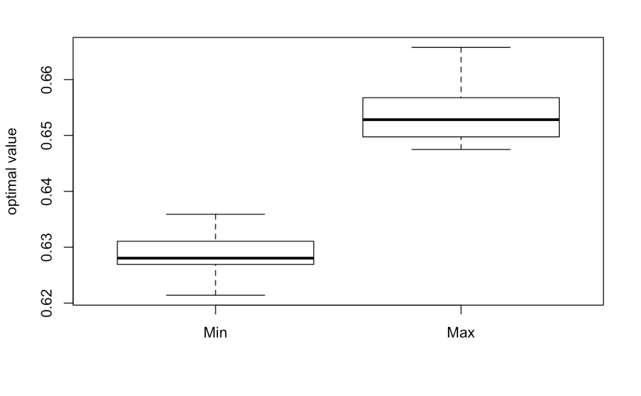
We then test the coverage of our obtained bounds. For this, we repeatedly sample new output data set of size for times. For each data set, we generate new support points of size . Then we run Algorithm 2. Out of intervals we obtained, five of them cover the true expected queue length. This gives us a confidence interval for the coverage probability , which is consistent with the theoretical guarantee provided by Theorem 4.2.
We have also tested the use of randomized stochastic projected gradient (RSPG), proposed by Ghadimi et al. (2016), that has been shown to perform well theoretically and empirically for problems with non-convex stochastic objectives. Specifically, we adapt the algorithm in Section 4.1 and 4.2 of Ghadimi et al. (2016) heuristically for the current problem we face that has stochastic non-convex constraints. Algorithm 4 in the appendix shows the adaptation of a single run procedure, and Algorithm 5 shows the adaptation of a post-optimization step to boost the final performance. In our algorithmic specification, we choose , , , , , and we fix at . We run Algorithm 5 for two realizations of data and support generation when the true service time distribution is exponential, with and . For each realization, we also run Algorithm 2 for comparison. For the first realization, we obtained using RSPG, compared with using Algorithm 2. For the second realization, we obtained using RSPG, compared with using Algorithm 2. The RSPG thus appears to perform very similarly as our procedure, at least for this particular setup (which shows that RSPG could be an alternative for future investigation).
We test the sensitivity of the algorithm with respect to the bounds in the constraints provided by the KS statistic. More concretely, in Algorithm 2, we increase the number in the constraint interval by a small . Table 2 shows that the obtained bounds are quite stable and do not show significant changes.
| perturbation size | min value | max value |
|---|---|---|
| 0.01 | 0.625 | 0.649 |
| 0.02 | 0.628 | 0.649 |
| 0.03 | 0.624 | 0.643 |
| 0.05 | 0.621 | 0.646 |
Finally, we test with a more “challenging” service time distribution that is an equally weighted mixture of two beta distributions with parameters and . This bimodal distribution has highest masses around and , with a shape shown in Figure 6.

We consider the setting with output observations. We randomly select input support points from uniform distribution in , and run Algorithm 2, using the same specifications as in the previous setup. The minimization stops at the value and the maximization stops at . These cover the true value (from running 1 million simulation using the true service time distribution). Thus our method appears to continue working in this case.
Figure 7 shows the minimal and maximal distributions from Algorithm 2. The distributions are quite spread out throughout the support, though the minimal distribution appears to have a noisy bimodal pattern. As we have discussed before, the shapes of these distributions should be interpreted as the worst-case distributions giving rise to the bounds, but are not indicative of the performance of our approach.


6.2 Inferring the Input Distribution Function
We now consider inferring the distribution function of the service time, i.e., for a range of values . We first use a true service time distribution that is exponential with rate . We consider a collection of observations from the average waiting time. We randomly generate support points from a lognormal distribution with and . We use Algorithm 2 with parameters , , .
Table 3 shows the obtained maximum and minimum values compared with the true distribution function evaluated at values ranging from to . Figure 8 further plots the trends of these values. The dashed lines represent the maximum and minimum values, and the solid line represents the true values. Note that Proposition 8.2, and the analogous extension of Theorem 4.2 to multiple objective functions discussed at the end of Section 4.2, allow us to compute the bounds for different values simultaneously with little sacrifice of statistical accuracy. In Table 3 and Figure 8, the obtained optimal values cover the truth at all points except the leftmost . This could be due to the challenge in inferring the tail (either left or right), stemming from perhaps the observed output we use (i.e., the waiting time) or the statistic we use to form our uncertainty set (i.e., the KS-statistic, which is known to not capture well the tail region of a distribution).
| min value | max value | true value | |
|---|---|---|---|
| 0.3 | 0.118 | 0.250 | 0.302 |
| 0.4 | 0.302 | 0.441 | 0.381 |
| 0.5 | 0.398 | 0.464 | 0.451 |
| 0.6 | 0.435 | 0.565 | 0.513 |
| 0.7 | 0.506 | 0.579 | 0.568 |
| 0.8 | 0.601 | 0.673 | 0.617 |
| 0.9 | 0.636 | 0.735 | 0.660 |
| 1 | 0.699 | 0.741 | 0.699 |
| 1.1 | 0.723 | 0.756 | 0.733 |
| 1.2 | 0.756 | 0.798 | 0.763 |

Figure 9 shows the minimal and maximal distributions for bounding when the algorithm terminates. We see that the shapes of both distributions resemble exponential, hinting that the service time distribution is close to identifiable in this case.


Next, we investigate the case when the true service time distribution is a mixture of two beta distributions with parameters and . We consider a collection of observations from the average waiting time. We randomly generate support points from a uniform distribution on .
Like in the previous case, Table 4 shows the maximum and minimum values from Algorithm 2, against the true values of at different values. Figure 10 further plots the trends of these values. Here, the obtained optimal values all cover the truth except at . The latter could be attributed to the statistical noise when running the many optimization procedures. The point is also one that could be “difficult” to infer intuitively, as it is in between the two modes. Nonetheless, our procedure appears to be reliable in general in bounding the distribution function across the domain of the service time.
| min value | max value | true value | |
|---|---|---|---|
| 0.2 | 0.129 | 0.231 | 0.188 |
| 0.25 | 0.208 | 0.266 | 0.267 |
| 0.3 | 0.262 | 0.358 | 0.337 |
| 0.35 | 0.296 | 0.395 | 0.393 |
| 0.4 | 0.362 | 0.413 | 0.435 |
| 0.45 | 0.389 | 0.464 | 0.466 |
| 0.5 | 0.416 | 0.503 | 0.491 |
| 0.55 | 0.504 | 0.577 | 0.516 |
| 0.6 | 0.509 | 0.594 | 0.548 |
| 0.65 | 0.573 | 0.611 | 0.591 |
| 0.7 | 0.628 | 0.679 | 0.649 |
| 0.75 | 0.678 | 0.736 | 0.722 |
| 0.8 | 0.724 | 0.834 | 0.805 |

Figure 11 shows the minimal and maximal distributions for bounding when the algorithm terminates. The shapes of these distributions are now considerably noisier than the exponential case in Figure 9. Nonetheless, there is a rough bimodal pattern (around and ).


7 Conclusion
We have studied an optimization-based framework to calibrate input quantities in stochastic simulation with only the availability of output data. Our approach uses an output-level uncertainty set, inspired by the DRO literature, to represent the statistical noise of the output data. By expressing the output distribution in terms of a simulable map of the input distribution, we can set up optimization programs cast over the input distribution that infers valid confidence bounds on the input quantities of interest.
We propose in particular an output-level uncertainty set based on the KS statistic, which exhibits advantages in computation (thanks to reformulation) and statistical accuracy (thanks to a controllable discretization scale needed to retain the confidence guarantee). We have shown these advantages via looking at the complexity of the resulting constraints and invoking the empirical process theory for -statistics. We also study a stochastic quadratic penalty method to solve the resulting optimization problems, including a convergence analysis that informs the suitable tuning of the parameters. Our numerical results demonstrate how our method could provide valid bounds for input quantities such as the input distribution function and other performance measures that rely on the input.
Acknowledgments.
A preliminary conference version of this work has appeared in Goeva et al. (2014). We gratefully acknowledge support from the National Science Foundation under grants CMMI-1542020, CMMI-1523453 and CAREER CMMI-1653339. We also thank Peter Haas for suggesting the use of quantile-based moments, and Russell Barton, Shane Henderson and Barry Nelson for other helpful suggestions.References
- Arcones and Gine (1993) Arcones MA, Gine E (1993) Limit theorems for u-processes. The Annals of Probability 1494–1542.
- Avellaneda et al. (2001) Avellaneda M, Buff R, Friedman C, Grandechamp N, Kruk L, Newman J (2001) Weighted Monte Carlo: a new technique for calibrating asset-pricing models. International Journal of Theoretical and Applied Finance 4(01):91–119.
- Balci and Sargent (1982) Balci O, Sargent RG (1982) Some examples of simulation model validation using hypothesis testing. Proceedings of the 14th Winter Simulation conference, volume 2, 621–629 (Winter Simulation Conference).
- Banks et al. (2009) Banks J, Carson J, Nelson B, Nicol D (2009) Discrete-Event System Simulation (Prentice Hall Englewood Cliffs, NJ, USA), 5th edition edition.
- Barton (2012) Barton RR (2012) Tutorial: Input uncertainty in outout analysis. Proceedings of the 2012 Winter Simulation Conference (WSC), 1–12 (IEEE).
- Barton et al. (2013) Barton RR, Nelson BL, Xie W (2013) Quantifying input uncertainty via simulation confidence intervals. INFORMS Journal on Computing 26(1):74–87.
- Barton and Schruben (2001) Barton RR, Schruben LW (2001) Resampling methods for input modeling. Proceedings of the 2001 Winter Simulation Conference, volume 1, 372–378 (IEEE).
- Basawa et al. (2008) Basawa I, Bhat U, Zhou J (2008) Parameter estimation using partial information with applications to queueing and related models. Statistics & Probability Letters 78(12):1375–1383.
- Basawa et al. (1996) Basawa IV, Bhat UN, Lund R (1996) Maximum likelihood estimation for single server queues from waiting time data. Queueing systems 24(1-4):155–167.
- Bayraksan and Love (2015) Bayraksan G, Love DK (2015) Data-driven stochastic programming using phi-divergences. The Operations Research Revolution, 1–19 (INFORMS).
- Beck and Teboulle (2003) Beck A, Teboulle M (2003) Mirror descent and nonlinear projected subgradient methods for convex optimization. Operations Research Letters 31(3):167–175.
- Ben-Tal et al. (2013) Ben-Tal A, Den Hertog D, De Waegenaere A, Melenberg B, Rennen G (2013) Robust solutions of optimization problems affected by uncertain probabilities. Management Science 59(2):341–357.
- Ben-Tal et al. (2009) Ben-Tal A, El Ghaoui L, Nemirovski A (2009) Robust optimization (Princeton University Press).
- Benveniste et al. (2012) Benveniste A, Métivier M, Priouret P (2012) Adaptive Algorithms and Stochastic Approximations, volume 22 (Springer Science & Business Media).
- Bertsekas (1999) Bertsekas DP (1999) Nonlinear programming (Athena Scientific).
- Bertsekas et al. (2003) Bertsekas DP, Nedi A, Ozdaglar AE, et al. (2003) Convex analysis and optimization .
- Bertsimas et al. (2011) Bertsimas D, Brown DB, Caramanis C (2011) Theory and applications of robust optimization. SIAM review 53(3):464–501.
- Bertsimas et al. (2014) Bertsimas D, Gupta V, Kallus N (2014) Robust saa. arXiv preprint arXiv:1408.4445 .
- Bertsimas and Natarajan (2007) Bertsimas D, Natarajan K (2007) A semidefinite optimization approach to the steady-state analysis of queueing systems. Queueing Systems 56(1):27–39.
- Bertsimas and Popescu (2005) Bertsimas D, Popescu I (2005) Optimal inequalities in probability theory: A convex optimization approach. SIAM Journal on Optimization 15(3):780–804.
- Bingham and Pitts (1999) Bingham N, Pitts SM (1999) Non-parametric estimation for the M/G/ queue. Annals of the Institute of Statistical Mathematics 51(1):71–97.
- Blanchet et al. (2016) Blanchet J, Kang Y, Murthy K (2016) Robust wasserstein profile inference and applications to machine learning. arXiv preprint arXiv:1610.05627 .
- Blanchet and Murthy (2016) Blanchet J, Murthy K (2016) Quantifying distributional model risk via optimal transport .
- Blum (1954) Blum JR (1954) Multidimensional stochastic approximation methods. The Annals of Mathematical Statistics 737–744.
- Bottou (1998) Bottou L (1998) Online learning and stochastic approximations. On-line learning in neural networks 17(9):142.
- Broadie et al. (2011) Broadie M, Cicek D, Zeevi A (2011) General bounds and finite-time improvement for the Kiefer-Wolfowitz stochastic approximation algorithm. Operations Research 59(5):1211–1224.
- Cheng and Holland (1998) Cheng RC, Holland W (1998) Two-point methods for assessing variability in simulation output. Journal of Statistical Computation Simulation 60(3):183–205.
- Cheng and Holland (2004) Cheng RC, Holland W (2004) Calculation of confidence intervals for simulation output. ACM Transactions on Modeling and Computer Simulation (TOMACS) 14(4):344–362.
- Chick (2001) Chick SE (2001) Input distribution selection for simulation experiments: accounting for input uncertainty. Operations Research 49(5):744–758.
- Chick and Ng (2002) Chick SE, Ng SH (2002) Simulation input analysis: joint criterion for factor identification and parameter estimation. Proceedings of the 34th Winter Simulation Conference, 400–406 (Winter Simulation Conference).
- Cooper (1972) Cooper RB (1972) Introduction to queueing theory .
- Csiszár (1991) Csiszár I (1991) Why least squares and maximum entropy? an axiomatic approach to inference for linear inverse problems. The Annals of Statistics 19(4):2032–2066.
- Currin et al. (1991) Currin C, Mitchell T, Morris M, Ylvisaker D (1991) Bayesian prediction of deterministic functions, with applications to the design and analysis of computer experiments. Journal of the American Statistical Association 86(416):953–963.
- Daley and Servi (1998) Daley D, Servi L (1998) Moment estimation of customer loss rates from transactional data. International Journal of Stochastic Analysis 11(3):301–310.
- Dang and Lan (2015) Dang CD, Lan G (2015) Stochastic block mirror descent methods for nonsmooth and stochastic optimization. SIAM Journal on Optimization 25(2):856–881.
- Delage and Ye (2010) Delage E, Ye Y (2010) Distributionally robust optimization under moment uncertainty with application to data-driven problems. Operations Research 58(3):595–612.
- Donoho et al. (1992) Donoho DL, Johnstone IM, Hoch JC, Stern AS (1992) Maximum entropy and the nearly black object. Journal of the Royal Statistical Society. Series B (Methodological) 41–81.
- Duchi et al. (2016) Duchi J, Glynn P, Namkoong H (2016) Statistics of robust optimization: A generalized empirical likelihood approach. arXiv preprint arXiv:1610.03425 .
- Durrett (2010) Durrett R (2010) Probability: Theory and Examples (Cambridge university press).
- Esfahani and Kuhn (2015) Esfahani PM, Kuhn D (2015) Data-driven distributionally robust optimization using the wasserstein metric: Performance guarantees and tractable reformulations. arXiv preprint arXiv:1505.05116 .
- Fan et al. (2013) Fan W, Hong LJ, Zhang X (2013) Robust selection of the best. Proceedings of the 2013 Winter Simulation Conference: Simulation: Making Decisions in a Complex World, 868–876 (IEEE Press).
- Fearnhead (2004) Fearnhead P (2004) Filtering recursions for calculating likelihoods for queues based on inter-departure time data. Statistics and Computing 14(3):261–266.
- Feng et al. (2014) Feng H, Dube P, Zhang L (2014) Estimating life-time distribution by observing population continuously. Performance Evaluation 79:182–197.
- Frey and Kaplan (2010) Frey JC, Kaplan EH (2010) Queue inference from periodic reporting data. Operations Research Letters 38(5):420–426.
- Gao and Kleywegt (2016) Gao R, Kleywegt AJ (2016) Distributionally robust stochastic optimization with wasserstein distance. arXiv preprint arXiv:1604.02199 .
- Ghadimi and Lan (2013) Ghadimi S, Lan G (2013) Stochastic first-and zeroth-order methods for nonconvex stochastic programming. SIAM Journal on Optimization 23(4):2341–2368.
- Ghadimi and Lan (2015) Ghadimi S, Lan G (2015) Accelerated gradient methods for nonconvex nonlinear and stochastic programming. Mathematical Programming 1–41.
- Ghadimi et al. (2016) Ghadimi S, Lan G, Zhang H (2016) Mini-batch stochastic approximation methods for nonconvex stochastic composite optimization. Mathematical Programming 155(1-2):267–305.
- Ghosh and Lam (2015a) Ghosh S, Lam H (2015a) Computing worst-case input models in stochastic simulation. Available at http://arxiv.org/pdf/1507.05609v1.pdf .
- Ghosh and Lam (2015b) Ghosh S, Lam H (2015b) Mirror descent stochastic approximation for computing worst-case stochastic input models. Proceedings of the 2015 Winter Simulation Conference, 425–436 (IEEE Press).
- Ghosh and Lam (2015c) Ghosh S, Lam H (2015c) Robust analysis in stochastic simulation: Computation and performance guarantees. arXiv preprint arXiv:1507.05609 .
- Glasserman and Xu (2013) Glasserman P, Xu X (2013) Robust portfolio control with stochastic factor dynamics. Operations Research 61(4):874–893.
- Glasserman and Xu (2014) Glasserman P, Xu X (2014) Robust risk measurement and model risk. Quantitative Finance 14(1):29–58.
- Glasserman and Yang (2016) Glasserman P, Yang L (2016) Bounding wrong-way risk in cva calculation. Mathematical Finance .
- Glasserman and Yu (2005) Glasserman P, Yu B (2005) Large sample properties of weighted Monte Carlo estimators. Operations Research 53(2):298–312.
- Goeva et al. (2014) Goeva A, Lam H, Zhang B (2014) Reconstructing input models via simulation optimization. Proceedings of the 2014 Winter Simulation Conference, 698–709 (IEEE Press).
- Goh and Sim (2010) Goh J, Sim M (2010) Distributionally robust optimization and its tractable approximations. Operations Research 58(4-Part-1):902–917.
- Gupta (2015) Gupta V (2015) Near-optimal ambiguity sets for distributionally robust optimization. Preprint .
- Hall and Park (2004) Hall P, Park J (2004) Nonparametric inference about service time distribution from indirect measurements. Journal of the Royal Statistical Society: Series B (Statistical Methodology) 66(4):861–875.
- Hanasusanto et al. (2017) Hanasusanto GA, Roitch V, Kuhn D, Wiesemann W (2017) Ambiguous joint chance constraints under mean and dispersion information. Operations Research 65(3):751–767.
- Hansen and Sargent (2008) Hansen LP, Sargent TJ (2008) Robustness (Princeton university press).
- Heckmüller and Wolfinger (2009) Heckmüller S, Wolfinger BE (2009) Reconstructing arrival processes to G/D/1 queueing systems and tandem networks. International Symposium on Performance Evaluation of Computer & Telecommunication Systems, 2009. SPECTS 2009., volume 41, 361–368 (IEEE).
- Hu et al. (2012) Hu Z, Cao J, Hong LJ (2012) Robust simulation of global warming policies using the dice model. Management science 58(12):2190–2206.
- Iyengar (2005) Iyengar GN (2005) Robust dynamic programming. Mathematics of Operations Research 30(2):257–280.
- Jain et al. (2010) Jain A, Lim A, Shanthikumar J (2010) On the optimality of threshold control in queues with model uncertainty. Queueing Systems 65:157–174.
- Kelton and Law (2000) Kelton WD, Law AM (2000) Simulation Modeling and Analysis (McGraw Hill Boston).
- Kennedy and O’Hagan (2001) Kennedy MC, O’Hagan A (2001) Bayesian calibration of computer models. Journal of the Royal Statistical Society: Series B (Statistical Methodology) 63(3):425–464.
- Kim and Park (2008) Kim YB, Park J (2008) New approaches for inference of unobservable queues. Proceedings of the 40th Conference on Winter Simulation, 2820–2825 (Winter Simulation Conference).
- Kleijnen (1995) Kleijnen JP (1995) Verification and validation of simulation models. European Journal of Operational Research 82(1):145–162.
- Kraan and Bedford (2005) Kraan B, Bedford T (2005) Probabilistic inversion of expert judgments in the quantification of model uncertainty. Management Science 51(6):995–1006.
- Lam (2013) Lam H (2013) Robust sensitivity analysis for stochastic systems. arXiv preprint arXiv:1303.0326 .
- Lam (2016) Lam H (2016) Recovering best statistical guarantees via the empirical divergence-based distributionally robust optimization. arXiv preprint arXiv:1605.09349 .
- Lam (2017) Lam H (2017) Sensitivity to serial dependency of input processes: A robust approach. Management Science .
- Lam and Mottet (2017) Lam H, Mottet C (2017) Tail analysis without parametric models: A worst-case perspective. Operations Research .
- Lam and Zhou (2017) Lam H, Zhou E (2017) The empirical likelihood approach to quantifying uncertainty in sample average approximation. Operations Research Letters 45(4):301–307.
- Lan and Zhou (2017) Lan G, Zhou Z (2017) Algorithms for stochastic optimization with expectation constraints. arXiv preprint arXiv:1604.03887 .
- Larson (1990) Larson RC (1990) The queue inference engine: Deducing queue statistics from transactional data. Management Science 36(5):586–601.
- Lehmann and Romano (2006) Lehmann EL, Romano JP (2006) Testing statistical hypotheses (Springer Science & Business Media).
- Li et al. (2016) Li B, Jiang R, Mathieu JL (2016) Ambiguous risk constraints with moment and unimodality information. Available at Optimization Online .
- Lim and Shanthikumar (2007) Lim AEB, Shanthikumar JG (2007) Relative entropy, exponential utility, and robust dynamic pricing. Operations Research 55(2):198–214.
- Mandelbaum and Zeltyn (1998) Mandelbaum A, Zeltyn S (1998) Estimating characteristics of queueing networks using transactional data. Queueing systems 29(1):75–127.
- Marjoram et al. (2003) Marjoram P, Molitor J, Plagnol V, Tavaré S (2003) Markov chain Monte Carlo without likelihoods. Proceedings of the National Academy of Sciences 100(26):15324–15328.
- Moulines et al. (2007) Moulines E, Roueff F, Souloumiac A, Trigano T (2007) Nonparametric inference of photon energy distribution from indirect measurement. Bernoulli 13(2):365–388.
- Nelson (2016) Nelson B (2016) ‘Some tactical problems in digital simulation’ for the next 10 years. Journal of Simulation 10(1):2–11.
- Nemirovski et al. (2009) Nemirovski A, Juditsky A, Lan G, Shapiro A (2009) Robust stochastic approximation approach to stochastic programming. SIAM Journal on Optimization 19(4):1574–1609.
- Park et al. (2011) Park J, Kim YB, Willemain TR (2011) Analysis of an unobservable queue using arrival and departure times. Computers & Industrial Engineering 61(3):842–847.
- Petersen et al. (2000) Petersen I, James M, Dupuis P (2000) Minimax optimal control of stochastic uncertain systems with relative entropy constraints. IEEE Transactions on Automatic Control 45(3):398–412.
- Pickands III and Stine (1997) Pickands III J, Stine RA (1997) Estimation for an M/G/ queue with incomplete information. Biometrika 84(2):295–308.
- Popescu (2005) Popescu I (2005) A semidefinite programming approach to optimal-moment bounds for convex classes of distributions. Mathematics of Operations Research 30(3):632–657.
- Ross et al. (2007) Ross JV, Taimre T, Pollett PK (2007) Estimation for queues from queue length data. Queueing Systems 55(2):131–138.
- Ryzhov et al. (2012) Ryzhov IO, Defourny B, Powell WB (2012) Ranking and selection meets robust optimization. Proceedings of the Winter Simulation Conference, 48 (Winter Simulation Conference).
- Santner et al. (2013) Santner TJ, Williams BJ, Notz WI (2013) The Design and Analysis of Computer Experiments (Springer Science & Business Media).
- Sargent (2005) Sargent RG (2005) Verification and validation of simulation models. Proceedings of the 37th Winter Simulation Conference, 130–143 (Winter Simulation Conference).
- Schruben (1980) Schruben LW (1980) Establishing the credibility of simulations. Simulation 34(3):101–105.
- Serfling (2009) Serfling RJ (2009) Approximation Theorems of Mathematical Statistics, volume 162 (John Wiley & Sons).
- Shafieezadeh-Abadeh et al. (2015) Shafieezadeh-Abadeh S, Esfahani PM, Kuhn D (2015) Distributionally robust logistic regression. Advances in Neural Information Processing Systems, 1576–1584.
- Shirangi (2014) Shirangi MG (2014) History matching production data and uncertainty assessment with an efficient TSVD parameterization algorithm. Journal of Petroleum Science and Engineering 113:54–71.
- Smith (1995) Smith JE (1995) Generalized Chebyshev inequalities: theory and applications in decision analysis. Operations Research 43(5):807–825.
- Song et al. (2014) Song E, Nelson BL, Pegden CD (2014) Advanced tutorial: Input uncertainty quantification. Proceedings of the 2014 Winter Simulation Conference, 162–176 (IEEE Press).
- Tarantola (2005) Tarantola A (2005) Inverse Problem Theory and Methods for Model Parameter Estimation (SIAM).
- Van Der Vaart and Wellner (1996) Van Der Vaart AW, Wellner JA (1996) Weak convergence. Weak convergence and empirical processes, 16–28 (Springer).
- Wang and Spall (2008) Wang IJ, Spall JC (2008) Stochastic optimisation with inequality constraints using simultaneous perturbations and penalty functions. International Journal of Control 81(8):1232–1238.
- Wang et al. (2006) Wang TY, Ke JC, Wang KH, Ho SC (2006) Maximum likelihood estimates and confidence intervals of an M/M/R queue with heterogeneous servers. Mathematical Methods of Operations Research 63(2):371–384.
- Whitt (1981) Whitt W (1981) Approximating a point process by a renewal process: The view through a queue, an indirect approach. Management Science 27(6):619–636.
- Whitt (1982) Whitt W (1982) Approximating a point process by a renewal process, I: Two basic methods. Operations Research 30(1):125–147.
- Whitt (2012) Whitt W (2012) Fitting birth-and-death queueing models to data. Statistics & Probability Letters 82(5):998–1004.
- Wiesemann et al. (2014) Wiesemann W, Kuhn D, Sim M (2014) Distributionally robust convex optimization. Operations Research 62(6):1358–1376.
- Wunsch (1996) Wunsch C (1996) The Ocean Circulation Inverse Problem (Cambridge University Press).
- Xu and Mannor (2012) Xu H, Mannor S (2012) Distributionally robust markov decision processes. Mathematics of Operations Research 37(2):288–300.
- Yu et al. (2017) Yu H, Neely M, Wei X (2017) Online convex optimization with stochastic constraints. Guyon I, Luxburg UV, Bengio S, Wallach H, Fergus R, Vishwanathan S, Garnett R, eds., Advances in Neural Information Processing Systems 30, 1427–1437 (Curran Associates, Inc.).
- Zouaoui and Wilson (2004) Zouaoui F, Wilson JR (2004) Accounting for input-model and input-parameter uncertainties in simulation. IIE Transactions 36(11):1135–1151.
Supplementary Materials
8 Proofs and Additional Results for Section 3
Proof 8.1
Proposition 8.2
Let and be the true input and output distributions. Consider a collection of quantities and the collection of optimization programs
| (40) |
and
| (41) |
for . Suppose is a confidence region for , i.e.,
where denotes the probability with respect to the data . Let be the set of optimal values of (40) and (41) respectively. Then we have
Similar statements hold if the confidence is approximate, i.e., if
then
9 Proofs for Section 4
Proof 9.1
Proof 9.2
Proof of Theorem 4.2. We will show the conclusion when (12) and (13) are replaced by
| (43) |
and
| (44) |
Then by the assumption that the true output distribution is continuous and that , we can use the same argument as in Theorem 4.1 to deduce that the constraints in (43) and (44) are equivalent to those in (12) and (13) with probability 1, from which we conclude the theorem.
Denote . Denote as the empirical distribution on given by
where is the delta mass on . Consider
i.e., is a discrete probability distribution with mass on each generated support point of . Consider, for any ,
| (45) | |||||
where is a measure (not necessarily a probability) given by
and the expectation is defined in a general sense as the -fold integral of with respect to . We consider both terms in (45). Writing , we can write the first term as
| (46) | |||||
Since , and by the definition of likelihood ratio, we have by the central limit theorem. By using the delta method (Chapter 3 in Serfling (2009)), we also have .
Moreover, is bounded by since . Hence (46) satisfies
| (47) |
Now consider the second term in (45). We have
by the definition of , and . Note that is the average, over all possible selections with replacement of drawn from , of the multilinear form . This is equivalent to the -statistic (Serfling (2009) Chapter 5) with kernel .
Define as the class of functions from to given by . Since is non-decreasing fixing each , and the envelope of , namely , is bounded by a.s., Problem 3 in Chapter 2.7 of Van Der Vaart and Wellner (1996) (Theorem 13.1 in the appendix) implies that has a polynomial bracketing number. Therefore, Theorem 4.10 in Arcones and Gine (1993) (Theorem 13.2 in the appendix; see also the discussion after therein) concludes the convergence
where is the -operator defined in (77) generated from , and is a Gaussian process defined as in (78).
Following the argument of the lemma in Section 5.7.3 in Serfling (2009), we can write the difference between the -statistic, denoted for simplicity , and the -statistic, denoted , as
where , and is the average of all where are drawn from with replacement and at least one overlapping selection. Following Serfling (2009), we can verify , and since , we have bounded a.s. Hence , and so .
Therefore, we write
where and converges to a Gaussian process. This entails that
| (48) |
From (45), and using (47) and (48), we get
| (49) | |||||
For the above chosen , we now have, for any small enough ,
| (50) | |||||
as and , where is a function with that satisfies , which exists by the continuity of the distribution of . The convergence (50) follows from the definition that is the true input distribution and hence is the true output distribution, thus leading to . It also follows from (49) so that as .
Similarly, for any small enough , we have
| (51) | |||||
as and . Since is arbitrary, by combining (50) and (51), we have
as and .
Lastly, we argue that the objective function satisfies . This follows mostly as a special case of the arguments above in showing , by simply replacing with and without considering the uniformity over . More precisely, we have
| (52) | |||||
similar to (45), where similar to (47), and by using the standard central limit theorem for -statistic (Theorem A in Section 5.5 in Serfling (2009)) and, with the assumption for any , translating it to -statistic (the lemma in Section 5.7.3 in Serfling (2009))). Therefore, we have .
We provide some remark on the case where we consider and for some collection of auxiliary input variate sequences that is independent of and has a known distribution. In this case, the results in Sections 3 and 4 all hold with the interpreted as the joint expectation taken with respect to both the product measure of and , the known distribution of . In the proofs above, we keep the expectation as taken under the product measure of only, but we use a conditioning argument, namely we change to and to , where and denote the conditional probability and expectation under the true distribution of given . In particular, in the proof of Theorem 4.2, we have that is non-decreasing given any , and , which, via Problem 3 in Chapter 2.7 of Van Der Vaart and Wellner (1996) again, gives a polynomial bracketing number for the class of functions . We also have for any , where denotes the joint expectation under the product measure of and , so that the central limit theorem for ensuring the approximation of the objective value holds in the proof. Other proofs follow quite trivially.
10 Proofs for Section 5
Proof 10.1
Proof of Proposition 5.1 Consider the equivalent reformulation of the program (14)
| (53) |
where both and are viewed as decision variables. An application of the conventional quadratic penalty method (Bertsekas (1999)) for equality constraints yields the following optimization sequence
| (54) |
for , which is equivalent to (15) with . Proposition 4.2.1 in Bertsekas (1999) entails that as (), every limit point of the sequence of optimal solutions to (54) is an optimal solution to (53), given that (53) is feasible. Note that due to optimality, the optimal slack variables must take the following form
where each is the projection defined in (17). Since projections are continuous maps, the operations of taking limit points and coordinate projection are interchangeable, i.e.
This allows translation of optimality of the limit point of to optimality of the limit point of . The desired conclusion follows.
Proof 10.2
Proof of Proposition 5.2. Part 1 and the expression for in part 2 come from a direct application of Ghosh and Lam (2015a) and Ghosh and Lam (2015b). We will prove (28) and (29) in part 2 only, but in the more general setting of differentiable functions of expectations. Let with be a performance function, where is a finite and deterministic time horizon, and be any differentiable function. By the chain rule
Similar to (27) we have
where
Therefore the following expression holds for the derivative
(28) and (29) follow from applying the above result to , and respectively, together with the linearity of differentiation. Note that .
Proof 10.3
Proof of Proposition 5.4.First note that the function is continuous and strictly increasing in the interval , and satisfies at the endpoints. So indeed there exists a unique that solves (38). Then we show (37) is indeed the optimal solution. Consider the Lagrangian
defined for and . Since (35) is a convex program with linear constraints and obviously Slater’s condition holds, by Proposition 6.2.5 and Proposition 6.4.4 of Bertsekas et al. (2003) it suffices to find dual variables and such that the solution given by (37) satisfies the set of KKT conditions
| (55) | ||||
| (56) | ||||
| (57) |
Equations (56) obviously hold because of equation (38). Equations (55) can be rewritten as
which hold if are chosen such that
It is obvious that such chosen . To show complementary slackness (57), note that if then (38) forces which results in .
Proof 10.4
Proof of Theorem 5.3.Consider the auxiliary programs obtained from replacing by some in (14)
and
Denote by and optimal solutions of the above maximization and minimization programs, which by Theorem 4.2 satisfy
Now, we try to show that and , therefore to conclude that
| (58) |
To avoid repetition, we only prove the minimization case here. To proceed, let be two arbitrary probability distributions in , and be the corresponding -fold product measure, then we have
where denotes the total variation distance between the product measures. It is well-known that the total variation distance between product measures can be bounded as (see, e.g. Lemma 3.6.2 of Durrett (2010))
therefore
Similarly for the constraint functions we have
Consider the total variation ball of radius surrounding
It is clear that for all it holds
| (59) | ||||
| (60) |
Note that is optimal and hence feasible for the program with , thus the inequality (60) ensures for all
Since , for large enough we have which results in
That is, all satisfy the first constraint in (33). In view of inequality (59), it remains to show that in order to conclude . Easily one can verify that for any it holds , and in particular which implies .
Lastly note that (58) holds true for arbitrary , hence holds for as well. This concludes the theorem.
Lemma 10.5
For any and , the moments of gradient estimators
are continuous in , the relative interior of .
Proof 10.6
Proof of Lemma 10.5.Restricted to , each of the moments can be written as the sum of finitely many terms each of which are smooth in . A sum of finitely many smooth functions is also smooth, hence continuous.
Lemma 10.7
Let be a positive sequence. If for and constants it holds for all large enough, then there exits a constant such that for all .
Proof 10.8
Proof of Lemma 10.7. Assume , then
Note that the above argument goes through when is large and is chosen such that , and . By induction holds for all sufficiently large . By enlarging one can make it hold for all .
Proof 10.9
Proof of Theorem 5.5. We borrow from Lemma 2.1 in Nemirovski et al. (2009) the inequality
| (61) |
which holds as long as is the prox-mapping of . The norm is the supremum norm, the dual of the -norm that is used in the strong convexity property of , with . Note that and both , by mean value theorem it holds
| (62) |
where is an absolute constant. This gives
| (63) |
Let be the filtration generated by . Taking conditional expectation of (63) with respect to , we have
| (64) |
Note that on the right hand side we are still using , the derivative of the quadratic penalty in the formulation (16), rather than .
In order to use the martingale convergence theorem, we examine the following
| (65) | ||||
We need to bound two quantities, and . To bound the first one
| (66) |
where in the first inequality we use Cauchy Schwartz inequality, and the third inequality holds because each by Lemma 10.5 is continuous in and hence by a compactness argument is uniformly bounded in . Therefore the key step lies in deriving an upper bound for each , for which we need the counterpart of (61) for , i.e.
Taking expectation with respect to gives
| (67) |
Note that with step size we have
where the second last inequality follows from
and in the last inequality we use Young’s inequality. Substituting the above into (67) gives
Hence taking full expectation we have the following recursion
Denote by . When the sequences and are taken to be (39), the recursion reduces to
which by Lemma 10.7 implies that . Therefore from (66) we conclude
| (68) |
To bound the term , we use Minkowski inequality to get
and
Again by Proposition 10.5, each expectation in the sum is continuous in , hence uniformly bounded in by compactness. Therefore and uniformly holds for some . This implies
| (69) |
Assumption 5.3 entails . Substituting (68) and (69) into (65) we arrive at
By martingale convergence theorem (Corollary in Section 3 in Blum (1954), restated in Theorem 13.3 in the Appendix), we have converges a.s. to some random variable . Because of and inequality (62) which holds uniformly for , we conclude that converges a.s. to the same variable .
Now we would like to argue that the limit a.s.. To this end it suffices to show that a.s. there exists a subsequence of converging to . Taking expectation and summing up on both sides of (76) and using similar bounding techniques, we have
Since each , it follows that
Define the (random) set of feasible-solution indices
Note that when is feasible for (33), it holds , hence
| (70) | ||||
| (71) |
If , then due to (70) there must exist a subsequence such that . Since , this implies that , which by Assumption 5.3 further implies that .
Otherwise if then it must hold because the parameters stated in the theorem satisfy . Due to (71) there exists a subsequence such that
| (72) |
By a compactness argument, there exists a subsubsequence such that converges to some . First we argue that must be feasible for (33). Since and are uniformly bounded, it is clear that and hold. Therefore the difference . On the other hand because is continuous. This means so must be feasible in view of Assumption 5.3. Then we argue in fact. If then by Assumption 5.3, and we derive a contradiction as follows. Recall that each is infeasible for (33) and , where vanishes since is feasible. We have
which contradicts (72).
The above argument shows that a.s. there exists a subsequence of converging to , hence the corresponding . Since we have proved above that converges a.s., the limit must be identically 0. Therefore, by Pinsker’s inequality, we have in total variation a.s.. This concludes the theorem.
As discussed at the end of Section 5, our results and algorithms still hold in the presence of a collection of auxiliary independent input processes distributed according to known distributions. Like in Sections 4 and 9, all proofs in this section still apply by invoking the same conditioning argument. Specifically, in Proposition 5.2 the expressions (27),(28),(29) are still valid with replaced by , so are the estimators (30),(31). In Lemma 10.5, the continuity of moments of gradient estimators can be similarly established by conditioning. For example, the moment is equal to , hence the same proof applies viewing as the performance measure. Similarly, the boundedness condition in Theorem 5.3 is made on instead.
11 An Alternate MDSA Algorithm and Some Further Discussion
Algorithm 3 shows an alternate MDSA algorithm that does not use slack variables, but at the expense of increasing the simulation replication size per iteration.
When applied to the (restricted) penalized minimization problem (16), MDSA solves the following optimization given a current iterate
| (73) |
where carries the gradient information of the target performance measure at , contains the gradient information of the quadratic penalty function in (16) at , and is the KL divergence defined in (19). The step-wise subproblem (73) without stochastic noise is also called the entropic descent algorithm (Beck and Teboulle (2003)). To make it a single-run procedure, we decrease the penalty coefficient as the iteration goes on, and thereby arrive at the following counterpart of (20)
| (74) |
Inspired by (28) in Proposition 5.2, we use the following estimator for the gradient of the penalty function
| (75) |
where and are independent copies of the i.i.d. input process generated under and are used simultaneously for all . Since we are using the plug-in estimator for the projection, in general (75) has a bias. In particular, the bias can be shown to vanish as slow as if is close to either or . Due to this biasedness, the batch size has to grow to in the course of iteration in order for the algorithm to converge properly.
Input: A small parameter , initial solution , a step size sequence , a penalty sequence , a sample size sequences , and sample sizes .
Iteration: For , do the following: Given ,
Theorem 11.1
Here are some discussions on the parameter choices of Algorithm 3. is a standard condition in SA which ensures that the effect of stochasticity will vanish eventually, whereas the condition is meant to eliminate the effect of biasedness of the gradient estimator (75). What is special about our MDSA is the condition . The rationale for this condition is as follows. When is feasible for (33), the gradient of the penalty function vanishes, i.e. , hence the effective step size in (74) is . Under the condition , the algorithm is able to fully explore the feasible set of (33).
The difference between Algorithm 2 and 3 lies in how the projection at the current iterate is estimated. Algorithm 3 computes the projection by directly simulating from scratch and substituting into the projection in each iteration, whereas Algorithm 2 iteratively updates the slack variables together with the decision variable in such a way that eventually each consistently estimates the projection .
We point out that both Algorithm 2 and 3 are essentially solving the formulation (16), despite the fact that the design of Algorithm 2 is mostly based on (15). The reason that neither of Algorithm 2 and 3 solves the formulation (15) has to do with the fact that algorithmically the formulation (15) with slack variables in general is not as well behaved as the formulation (16) with the projections, despite their mathematical equivalence. To see this, consider a generic inequality constraint where is some decision variable. It is easy to see that the quadratic penalty expressed via projection preserves the convexity of , whereas the one with slack variable , , can very likely lose convexity even if itself is convex. In fact, if is jointly convex in and , is guaranteed to be convex. This also explains why the general convexity criterion in Assumptions 5.3 and 5.3 is imposed on formulation (16).
Proof 11.2
Proof of Theorem 11.1. The proof resembles that of Theorem 5.5. Let be the filtration generated by . Following the same line of argument, we have the following counterpart of (64)
| (76) |
We need to bound and . By independence of and and conditional Jensen’s inequality
where in the second last inequality we use the contraction property of projection, i.e. for any . The first inequality holds because each derivative by Proposition 10.5 is continuous in and by a compactness argument is hence uniformly bounded in . Following the proof of Theorem 5.5, one can show that
as the counterpart of (69).
12 A Randomized Stochastic Projected Gradient Algorithm for the Comparison in Section 6
We show a randomized stochastic projected gradient (RSPG) algorithm that we compare with in the numerical section. Algorithm 4 shows the procedure for a single run. Algorithm 5 includes a post-optimization step to boost its performance. As a rough guidance, we use where is the Lipschitz constant of the gradient function, and (the here could possibly be removed), where is the dimension of the decision space. could be a small number like , and the post-optimization batch size is chosen to be some big number. The penalty is chosen small and fixed.
Input: A small parameter , initial solution and , step size for both and , penalty , batch size , and number of iterations .
Generate random stopping time: Draw uniformly from
Iteration: For do the following: Given ,
Output:
Input: A small parameter , initial solution and , step size for both and , penalty , batch size , number of RSPG runs , and number of iterations per run. Batch size in the post-optimization phase.
Output: the where
13 Auxiliary Results
13.1 Results on Empirical Processes and -Statistics
We first introduce some definitions. Using Definition 2.1.6 in Van Der Vaart and Wellner (1996), given two functions and , the bracket is defined as the set of all functions with . An -bracket is a bracket with for some norm . For a class of measurable functions on , the bracketing number is the minimum number of -brackets needed to cover . Moreover, define the envelope of as .
We have the following theorem:
Theorem 13.1 (Problem 3 in Chapter 2.7 of Van Der Vaart and Wellner (1996))
Let be a class of measurable functions on , indexed by , such that is monotone for each . If the envelope function of is square integrable, then the bracketing number of is polynomial.
To introduce the next theorem, we define several additional notions. For any function , and generated i.i.d. from , define the -operator by
| (77) |
where . For convenience we denote , where is the expectation with respect to the -fold product measure of .
We say that a central theorem holds for if
| (78) |
where is the space (for functionals on ) defined by
is a Gaussian process indexed by that is centered and has covariance function
where is defined by and
where the sum is taken over all permutations of . Moreover, the process is sample continuous with respect to the canonical semi-metric
where is taken with respect to the probability . These discussions follow from Arcones and Gine (1993). We have ignored some measurability issues; see Van Der Vaart and Wellner (1996) for more details.
We have the following theorem:
Theorem 13.2 (Theorem 4.10 in Arcones and Gine (1993))
Let be a class of functions on . If
where is the norm induced in the -space under , the -fold product measure of . Then the central limit theorem holds for in the sense of (78).
13.2 Results Needed in the Convergence Proofs of the MDSA
Theorem 13.3 (Corollary in Section 3 in Blum (1954))
Let be a sequence of integrable random variables that satisfy
where if and 0 otherwise, and are bounded below uniformly in . Then converges a.s. to a random variable.