Detailed study of geodesics in the Kerr-Newman-(A)dS spactime and the rotating charged black hole spacetime in gravity
Abstract
We perform a detailed study of the geodesic equations in the spacetime of the static and rotating charged black hole corresponding to the Kerr-Newman-(A)dS spacetime. We derive the equations of motion for test particles and light rays and present their solutions in terms of the Weierstrass , and functions as well as the Kleinian function. With the help of parametric diagrams and effective potentials we analyze the geodesic motion and classify the possible orbit types. This spacetime is also a solution of gravity with a constant curvature scalar.
I INTRODUCTION
A large body of observational evidence has been gathered in support of an accelerated expansion of the universe at the present time. This includes, in particular, measurements of the luminosity distance of type Ia supernovae [1], the anisotropy of the cosmic microwave background [2, 3], weak lensing [4], baryon acoustic oscillations [5], and the large scale structure of the universe [6].
To explain the current accelerated expansion of the Universe is one of the most challenging problems of modern cosmology. In the current cosmological standard model, the CDM model, a small positive cosmological constant is included in the Einstein field equations to model this acceleration. It is therefore clearly of considerable interest, to study the influence of a cosmological constant on further solutions of the Einstein equations, such as black hole spacetimes, in particular.
For a deeper understanding of the gravitational field of massive objects and in order to accurately predict observational effects (such as light deflection, gravitational time delay, perihelion shift and Lense-Thirring effect), it is mandatory to have very good knowledge of the motion of test particles and light rays in the spacetimes of interest. But only analytical methods allow for arbitrarily high accuracy of the prediction of this motion and the associated observables.
In the Schwarzschild spacetime the equations of motion of test particles and light rays were solved analytically in terms of elliptic functions by Hagihara in 1931 [7]. The geodesic equations in the Reissner-Nordström, Kerr, and Kerr-Newman space-times have the same mathematical structure [8] and can be solved analogously. This analytical method was recently further advanced and applied to the hyperelliptical case, where the analytical solution of the equations of motion in the 4-dimensional Schwarzschild-(A)dS, Reissner-Nordström-(A)dS and Kerr-(A)dS spacetimes was presented [9, 10, 11, 12, 13, 14].
These mathematical tools were also applied to the geodesic motion in Taub-NUT and wormhole spacetimes [15, 16], and to higher dimensional spacetimes, including static black hole spacetimes and Myers-Perry spacetimes [10, 17, 18, 19], while in five dimensional black ring spacetimes, the equations of motion could be solved analytically in special cases [20, 21]. Moreover, the motion of test particles was studied in various black string spacetimes including field theoretical cosmic string spacetimes and black holes pierced by a black string [22, 23, 24, 25, 26, 27, 28, 29]. In addition, the geodesic equations were solved analytically in a static black hole spacetime of gravity [30], for Hořava-Lifshitz black holes [31], and for BTZ and GMGHS black holes [32, 33].
On the other hand, the large body of current cosmological data could also be taken to indicate that General Relativity itself should be extended. The latter would also be supported by the necessity for dark matter as revealed from astrophysical and cosmological observations (see e.g. [34]) and moreover by theoretical arguments at the ultraviolet scale (e.g., quantum gravity, initial singularities).
Consequently, numerous theoretical attempts to model the evolution of the Universe are based on the modification of gravity (see e.g. the reviews [35, 36, 37, 38, 39]). Popular suggestions to modify gravity include theories with higher powers of the Riemann and Ricci tensors as well as the curvature scalar . Lovelock theory [40] and gravity [41, 42, 35] are such examples, where the Einstein-Hilbert action is generalized accordingly.
A change of the action has influence on the dynamics of the Universe, but it may also affect the dynamics at the galactic or solar system scales. Clearly, any modifications of the action must retain the well tested sector of General Relativity, like its description of the solar system. However, modified theories may yield different answers from General Relativity in the strong field regime. It is therefore essential to inquire about the existence of black holes and about their properties in modified theories of gravity (see e.g. [43]). In general, the study of black holes in these theories may reveal interesting features not present in General Relativity.
Focussing on black holes in theories [44, 45, 46, 47, 48, 49, 53, 50, 51, 52, 54], we note that a particular class of solutions is obtained when the curvature scalar is constant, . Taking the trace of the field equations then specifies this constant in terms of the function and its derivative at . A comparison with General Relativity and its black hole solutions reveals, that the finite curvature scalar acts basically like a cosmological constant. In vacuum therefore the Schwarzschild-(A)dS and Kerr-(A)dS solutions are recovered, when certain rescalings are performed. When adding charge to the solutions by including an electromagnetic field, the Reissner-Nordström-(A)dS and the Kerr-Newman–(A)dS solutions can be recovered after certain rescalings, because the trace of the energy momentum tensor vanishes.
In this paper we study the geodesic motion in the spacetime of the static and rotating charged black hole (Kerr-Newman-(A)dS spacetime). Since after certain rescalings the Kerr-Newman-(A)dS black hole of General Relativity also describes a rotating charged black hole in gravity, the current analysis can also be applied to this black hole solution in gravity. Let us mention, however, that the stability of this black hole can only be established, after the function is specified.
We here analyze the possible orbit types using effective potential techniques and parametric diagrams. Furthermore, we present the analytical solutions of the equations of motion for test particles and light. The equations of motion are of elliptic and hyperelliptic type and the solutions are given in terms of the Weierstrass , and functions as well as the Kleinian functions. Complete integrability of the geodesic equations is guaranteed by the presence of four integrals of motion of the Kerr-Newman-(A)dS spacetime, with the forth one being the Carter constant.
Similar analyses of geodesic motion and solutions of the equations of motion were presented in the Kerr-(A)dS spacetime [12] and in the Kerr-Newman spacetime [55], but in the Kerr-Newman-(A)dS spacetime the geodesic motion has not been analyzed analytically before in great detail, although some aspects were studied in [57, 56]. The analytical solution of the geodesic equation of light and a study of the gravitational lensing and frame dragging of light were presented in [58]. However, neither an analysis of all possible orbits for particles and light was done nor the full set of analytic solutions to the equations of motions was found.
Our paper is organized as follows: In Sec. (II) we give a brief review of the field equations and the metric of the rotating black hole in gravity and its connection to General Relativity. In Sec. (III) we present the equations of motion in the Kerr-Newman-(A)dS spacetime. We analyze the geodesic motion in Sec. (IV) and give a list of all possible orbit types. The analysis is given separately for the static case (Reissner-Nordström-(A)dS) and the rotating case (Kerr-Newman-(A)dS). In Sec. (V) we present the full set of analytical solutions of the geodesic equations in the general rotating case of the Kerr-Newman-(A)dS black hole. Some example orbits in the static and the rotating case are shown in Sec. (VI). We conclude in Sec. (VII).
II FIELD EQUATIONS IN MODIFIED GRAVITY AND RESCALINGS
In this section we give a brief review of the field equations and the metric of the rotating black hole in , which represents the Kerr-Newman-(A)dS spacetime after certain rescalings. In four dimensions the action of gravity with a Maxwell field is given by
| (1) |
where and are the gravitational and the electromagnetic actions
| (2) |
| (3) |
where is the gravitational constant, which we will set to one, is the determinant of the metric, is the curvature scalar, and is the function defining the modified gravity theory under consideration. From the above action, the Maxwell equations take the form
| (4) |
while the field equations in the metric formalism are
| (5) |
where is the Ricci tensor, denotes the usual covariant derivative, and the stress-energy tensor of the electromagnetic field is given by
| (6) |
and has vanishing trace
| (7) |
Taking the trace of Eq. (5) under the assumption, that the curvature scalar is constant, , leads to
| (8) |
This is the same equation as in the vacuum case, because the matter field has vanishing trace, Eq. (7), and it determines the constant value of the curvature scalar
| (9) |
Using this relation in Eq. (5) gives the field equations
| (10) |
Comparison with the Einstein equations in the presence of a cosmological constant then indicates an equivalence of the two sets of equations for , when we further rescale the left hand side of the equations adequately.
Consequently, up to rescalings, the Kerr-Newman-(A)dS solution of General Relativity is also a solution of the field equations in gravity [50, 51, 52]. Thus, the stationary black hole solution can be obtained in Boyer-Lindquist like coordinates as follows [50]
| (11) |
with
| (12) |
| (13) |
where is the electric charge, is the angular momentum per mass of the black hole, and enters like a cosmological constant (), yielding a non-asymptotically flat de Sitter or anti-de Sitter spacetime, when is finite. Note, that the electric charge enters with a scaling factor in the metric. As in the Kerr spacetime there is a ringlike singularity defined by , and the horizons are given by .
III THE GEODESIC EQUATIONS
In this section we derive the equations of motion for a rotating charged black hole Eq.(11), using the Hamilton-Jacobi formalism, and later introduce effective potentials for the - and -motion.
The Hamilton-Jacobi equation
| (14) |
can be solved with an ansatz for the action
| (15) |
The constants of motion are the energy and the angular momentum which are given by the generalized momenta and
| (16) |
| (17) |
where each side depends on or only. With the separation ansatz Eq.(15) and with the help of the Carter constant [59], we derive the equations of motion:
| (18) |
| (19) |
| (20) |
| (21) |
In the following we will explicitly solve these equations. Eq.(18) suggests the introduction of an effective potential such that corresponds to
| (22) |
where for and . In the same way an effective potential corresponding to Eq.(19) can be introduced
| (23) |
but here for .
Introducing the Mino time [60] connected to the proper time
by , the equations of motions read
| (24) |
| (25) |
| (26) |
| (27) |
we introduce dimensionless quantities to rescale the parameters
| (28) |
Then the equations (24) - (27) can be rewritten as
| (29) |
| (30) |
| (31) |
| (32) |
IV ANALYSIS OF THE GEODESIC EQUATIONS
In this section we will analyze the geodesic equations and give a list of all possible orbits. First we will study the special case of a static charged black hole (Reissner-Nordström-(A)dS) and then we will give a full analysis of the general rotating charged black hole solution (Kerr-Newman-(A)dS).
IV.1 The static case
In this section, we investigate the possible orbit types in the static case with the help of the analytical solutions which are described in previous sections, parameter diagrams (see Fig.1) and the effective potential (see Fig.2).
In the static case the motion is confined to a plane and therefore the geodesic equations reduce to
| (33) |
| (34) |
where we introduced . An effective potential can be defined as
| (35) |
The shape of an orbit depends on the energy and the angular momentum of the test particle or light ray, as well as the charge and the cosmological constant . The mass can be absorbed through a rescaling of the radial coordinate and the parameters
| (36) |
Thus, Eq. (33) can be written as
| (37) |
In following we give a list of the possible orbits types. Let be the inner horizon and be the outer event horizon.
- 1.
Escape orbit (EO) with range where .
- 2.
Two-world escape orbit (TEO) with range where .
- 3.
Bound orbit (BO) with range with .
- 4.
Many-world bound orbit (MBO) with range where and .
- 5.
Terminating orbit (TO) with ranges
- (a)
either (Terminating escape orbit – TEO)
- (b)
or with (Terminating bound orbit – TBO).
TOs only occur for , otherwise the charge will provide a potential barrier preventing the geodesic from reaching the singularity at .
- (a)
These five regular types of geodesic motion correspond to different arrangements of the real and positive zeros of defining the borders of or, equivalently, .
Eq. (37) implies that is a necessary condition for the existence of a geodesic and, thus, that the positive zeros of are the turning points of the orbits. If for a given set of parameters the polynomial has positive zeros, then for varying and this number can only change if two zeros merge to one. Solving for and , for , yields
| (38) |
and for , yields
| (39) |
In Fig. 1, the results of this analysis are shown for both test particles () and light rays ().


In the Parametric --diagrams three regions of geodesic motion with different numbers of zeros can be identified (in the following is assumed):
- 1.
Region I:
- (a)
: has a single positive real zero and for . The only possible orbit type is EO.
- (b)
: has two positive zeros and for . The only possible orbit type is MBO.
- (a)
- 2.
Region II:
- (a)
: has three positive zeros with for and . Possible orbit types are MBO and EO.
- (b)
: has two positive zeros and for . The only possible orbit type is MBO.
- (a)
- 3.
Region III:
- (a)
: has five positive zeros with for , and . Possible orbit types are MBO, BO and EO.
- (b)
: has four positive zeros with for and . Possible orbit types are MBO and BO.
- (a)
Terminating orbits are possible in all three regions iff the black hole is uncharged . For light rays only regions I and II appear and therefore stable bound orbits do not exist for . A summary of possible orbit types for and can be found in Tables 1 and 2 respectively.
| zeros | region | range of | orbit |
|---|---|---|---|
| 1 | I | -2.5,-0.2)(4,0.2) | TEO |
| 3 | II | -2.5,-0.2)(4,0.2) | MBO, EO |
| -2.5,-0.2)(4,0.2) | MBO, EO | ||
| 5 | III | -2.5,-0.2)(4,0.2) | MBO, BO, EO |
| zeros | region | range of | orbit |
|---|---|---|---|
| 2 | I, II | -2.5,-0.2)(4,0.2) | MBO |
| II | -2.5,-0.2)(4,0.2) | MBO | |
| 4 | III | -2.5,-0.2)(4,0.2) | MBO, BO |
For a plot of the effective potential introduced in Eq.(35) with example energies corresponding to the different regions is shown in Fig 2. Here the possible orbit types can be identified.


IV.2 The rotating case
In this section we analyse the equations of motion in the rotating case (Kerr-Newman-(A)dS spacetime) and investigate the possible orbit types.
IV.2.1 Types of latitudinal motion
In this subsection and the next subsection, we use the function in Eq. (30) and the polynomial in Eq. (29), to determine the possible orbits of light and test particles.
First we substitute with in the function :
| (40) |
Geodesic motion is possible if , then real values of the coordinate are obtained. This condition also implies that for all geodesics with , or . From the observational side is always true, since the cosmological constant acquires a very small positive value.
The number of zeros of , which are the turning points of the latitudinal motion, only changes if a zero crosses or , or if a double zero occurs. is a zero of if
| (41) |
and therefore
| (42) |
Since is a pole of for , it is only possible that is a zero of if ,
| (43) |
To remove the pole of at we consider
| (44) |
where . Then double zeros fulfill the conditions
| (45) |
which yields
| (46) |
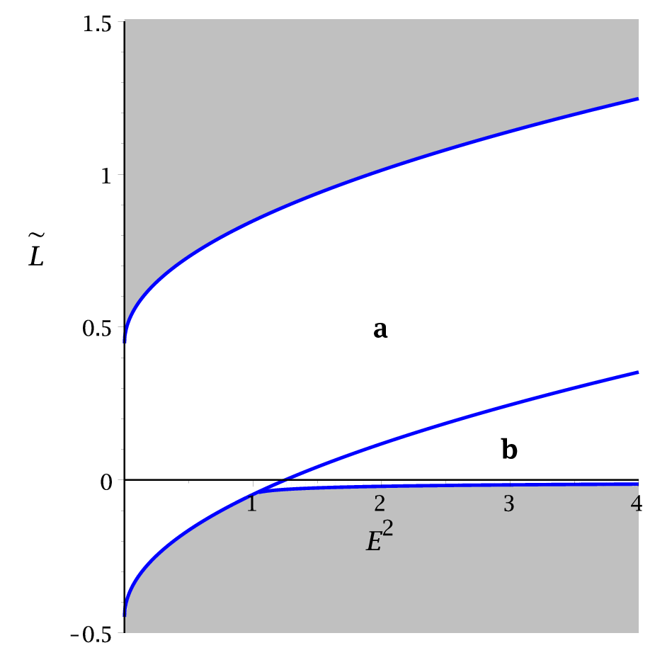
From the condition of being a zero and the condition of double zeros, we can plot parametric --diagrams, see figure 3. These reveal two regions in which geodesic motion is possible. The function has a single zero in region a, therefore the geodesics will cross the equatorial plane (). In region b, the function has two zeros , , which corresponds to motion above or below the equatorial plane (). If , the geodesics will reside in the equatorial plane.
IV.2.2 Types of radial motion
The zeros of the polynomial are the turning points of orbits of light and test particles, and therefore determines the possible types of orbits
| (47) |
with
| (48) |
where we introduced
| (49) |
There are bound orbits, where test particles move back and forth between two turning points, and escape orbits, where the black hole is approached, but the test particles turn around at a certain point to escape towards infinity. Terminating orbits end in the singularity, if they reach simultaneously and , such that . If a test particle crosses the black hole horizons twice or even multiple times, it can enter another universe. These orbits are called two-world orbits or many-world orbits. Due to the ring singularity it is possible that a geodesic crosses , which is then called transit orbit or crossover orbit [12]. Below we give a list of all possible orbits. Let be the outer event horizon and be the inner horizon of the black hole:
- 1.
Transit orbit (TrO) with range .
- 2.
Escape orbit (EO) with range with , or with range with .
- 3.
Two-world escape orbit (TEO) with range where .
- 4.
Crossover two-world escape orbit (CTEO) with range where .
- 5.
Bound orbit (BO) with range with
- (a)
or
- (b)
- (a)
- 6.
Many-world bound orbit (MBO) with range where and .
- 7.
Terminating orbit (TO) with ranges either or with
- (a)
or
- (b)
- (a)
The type of an orbit is determined by the number of real zeros of the polynomial . This number changes if a double zero occurs
| (50) |
Additionally the distinction between positive () and negative () zeros is interesting, since the geodesics can cross . The number of positive and negative zeros changes if . Taking both these conditions into account, we can plot parametric --diagrams, which show five regions with different numbers of zeros. In region I has no zeros. In region II there are two negative zeros. A negative and a positive zero are possible in region III. Region IV has three positive and a single negative zero. Five positive zeros and a negative zero appear in region V. In figure 4 examples of the parametric --diagrams of the -motion can be seen. We combined them with the parametric diagrams of the -motion.
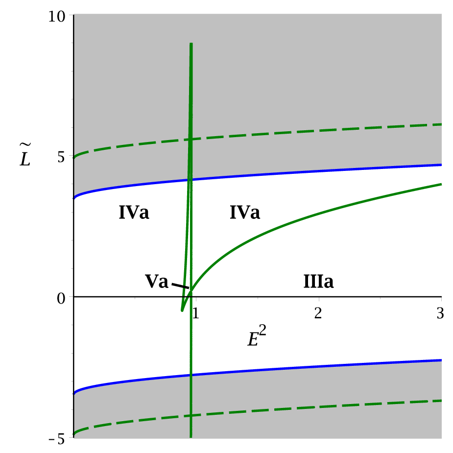
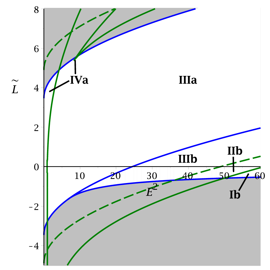
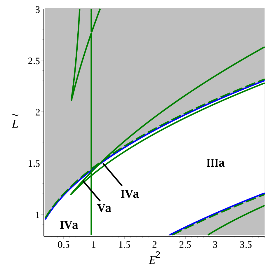
The regions I and II intersect only with region b so here the orbits will not cross the equatorial plane. The regions IV and V only intersect with region a, therefore the orbits will cross the equatorial plane. Region III intersects both with the regions a and b. In the regions I and II the geodesics can cross , but in the regions III, IV and V cannot be crossed.
We conclude that the only way for a geodesic to reach the singularity (Terminating Orbit) is and . This is the case if and additionally .
We use the parametric --diagrams and the effective potential of the -equation (see figure 5) to determine all possible orbit types. Table 3 shows an overview. If null geodesics () are considered, the region V vanishes from the parametric --diagrams, therefore orbits of type F and G (see table 3) are not possible for light. This implies that bound orbits outside the horizons () are only possible for particles but not for light.


The preceding analysis was done for which implies a positive cosmological constant. Since the motion of test particles and light in this spacetime is similar to the Kerr-(A)dS spacetime we refer to [12] for an analysis concerning a negative cosmogical constant. In comparison with the parametric diagrams of [12] it is obvious that the overall behaviour and the possible orbit types are the same, still, there are some differences to the Kerr-(A)dS spacetime caused by the parameter . In the spacetime of a rotating black hole, there are orbits that do not cross and also do not cross the equatorial plane (). This occurs in the region IIIb (see figure 4 and table 3), which is not present for the Kerr-(A)dS case . In the Kerr-(A)dS spacetime the green dashed line in figure 4 will coincide with the blue lines from the parametric plot, so that region III is not splitted into an a and a b part. Therefore, in the Kerr-(A)dS case an orbit that crosses will not cross and an orbit that crosses will not cross .
A further difference to the Kerr case is that terminating orbits do not exist for . Only orbits with and simultaneously end in the singularity.
| type | zeros | region | range of | orbit |
| A | 0 | Ib | -4,-0.2)(3.5,0.2) | TrO |
| B | 2 | IIb | -4,-0.2)(3.5,0.2) | EO, CTEO |
| C | 2 | IIIa,b | -4,-0.2)(3.5,0.2) | EO, TEO |
| C- | -4,-0.2)(3.5,0.2) | EO, TEO | ||
| C0 | -4,-0.2)(3.5,0.2) | EO, TO/TEO | ||
| D | 4 | IVa | -4,-0.2)(3.5,0.2) | EO, MBO, EO |
| D- | -4,-0.2)(3.5,0.2) | EO, MBO, EO | ||
| D+ | -4,-0.2)(3.5,0.2) | EO, MBO, EO | ||
| D± | -4,-0.2)(3.5,0.2) | EO, MBO, EO | ||
| D0 | -4,-0.2)(3.5,0.2) | EO, TO/MBO, EO | ||
| D | -4,-0.2)(3.5,0.2) | EO, TO/MBO, EO | ||
| E | 4 | IVa | -4,-0.2)(3.5,0.2) | EO, BO, TEO |
| E- | -4,-0.2)(3.5,0.2) | EO, BO, TEO | ||
| E0 | -4,-0.2)(3.5,0.2) | EO, TO/BO, TEO | ||
| E | -4,-0.2)(3.5,0.2) | EO, TO/BO, TEO | ||
| F | 6 | Va | -4,-0.2)(3.5,0.2) | EO, MBO, BO, EO |
| F- | -4,-0.2)(3.5,0.2) | EO, MBO, BO, EO | ||
| F+ | -4,-0.2)(3.5,0.2) | EO, MBO, BO, EO | ||
| G | 6 | Va | -4,-0.2)(3.5,0.2) | EO, BO, MBO, EO |
| G- | -4,-0.2)(3.5,0.2) | EO, BO, MBO, EO | ||
| G0 | -4,-0.2)(3.5,0.2) | EO, TO/BO, MBO, EO | ||
| G | -4,-0.2)(3.5,0.2) | EO, TO/BO, MBO, EO |
V ANALYTICAL SOLUTION OF THE GEODESIC EQUATIONS
In this section, we will present the analytical solutions of the geodesic equations (29)–(32) in the Kerr-Newman-(A)dS spacetime. We will treat each equation separately and give the solutions in terms of the Weierstrass , and functions as well as the Kleinian function.
V.1 motion
We start with the differential equation (30) describing the motion
| (51) |
and substitute to simplify the equation
| (52) |
V.1.1 Timelike geodesics
The differential equation (52) is of elliptic type, since is in general a polynomial of order four. Here we consider the case . Assuming that has only simple zeros, equation (52) can be solved in terms of the Weierstrass elliptic function. To get the solution we transform into the Weierstrass form with the constants and . First, we apply the substitution yielding
| (53) |
where
| (54) |
is a now a polynomial of order three. Second, we substitute , which gives
| (55) |
where the Weierstrass invariants are
| (56) |
| (57) |
The differential equation (55) represents an elliptic intregal of the first kind, which can be solved by [9, 61, 62]
| (58) |
Finally, the solution of Eq.(30) is given by
| (59) |
where and depends only on the initial values and . Since the motion is symmetric with respect to the equatorial plane , the sign of the square root can be chosen so that is either in (positive sign) or in (negative sign).
V.1.2 Null geodesics
V.2 r motion
The dynamics of are described by the differential equation (29)
| (61) |
Here the solution procedure is more complicated because is in general a polynomial of order six. However, for null geodesics the order of the polynomial is reduced to four. In the following we will consider timelike and null geodesics separately.
V.2.1 Null geodesics
Considering light, i.e. , is simplified to a polynomial of degree four and therefore the differential equation (29) is of elliptic type. Then we can solve it using the method of section V.1. By substituting first , where is a zero of , and then , where , Eq. (29) aquires the form of Eq. (55). Again, this can be solved with the help of the Weierstrass elliptic function, so that the result is
| (62) |
where and depends only on the initial values and and , are defined as in Eq.(57) with .
V.2.2 Timelike geodesics
Considering particles, i.e. , and assuming that has only simple zeros, the differential equation (29) is of hyperelliptic type. As presented in [12], this equation can be solved in terms of derivatives of the Kleinian function. To begin with, Eq. (29) is transformed into the standard form with the substitution where is a zero of . Then we get
| (63) |
where
| (64) |
A separation of variables leads to
| (65) |
where . Considering the solution of the integral (65), we have to address two points. First, due to the two branches of the square root the integrand is not well defined in the complex plane. Second, the solution should not depend on the chosen path of integration [9]. Let be a closed integration path and
| (66) |
then also
| (67) |
should be true. Hence, the solution of our problem has to fulfill
| (68) |
for every obtained from Eq. (66). These two issues can be solved if we consider Eq. (65) to be defined on the Riemann surface of genus and introduce a basis of canonical holomorphic and meromorphic differentials and , respectively,
| (69) |
| (70) |
and real , and imaginary , period matrices
| (71) |
| (72) |
The equation (65) is a hyperelliptic integral of the first kind and can be solved by [12, 14]
| (73) |
where is the -th derivative of the Kleinian function
| (74) |
which is given by the Riemann -function with characteristic ,
| (75) |
A number of parameters enter here: the symmetric Riemann matrix , the period-matrix , the period-matrix of the second kind , the matrix , and the vector of Riemann constants with base point at infinity . The constant can be given explicitly, see e.g. [63], but is not important here. In Eq.(73) the argument is an element of the one-dimensional divisor: with and depends only on the initial values and , and the function can be found from the vanishing condition [12], so it describes the -divisor. Then the solution of the equation is given by
| (76) |
Here the sign depends on the sign that was chosen in the substitution . The functions and depend on and also on the polynomial according to Eqs. (), which contains all the parameter-dependence of the modified gravity solution. The solution of is the analytic solution of the equation of motion of a test particle in the Kerr-Newman-(A)dS spacetime. This solution is valid in all regions of this spacetime.
V.3 motion
The -equation (31) can be rewritten using the - and -equations, (29) and (30)
| (77) |
Intergrating this equation gives an -dependent integral and a -dependent integral which can be solved separately
| (78) |
V.3.1 The -dependent integral
Let us first consider the -dependent integral
| (79) |
which can be simplified by the substitution
| (80) |
where the polynomial is given in Eq. (44) and . Assuming has only simple zeros and is a polynomial of order four, then is an elliptic integral of the third kind. In this case the solution to is given by [12]
| (81) |
where the coefficients of the polynomial are given in subsection V.1 and
| (82) |
Also we have , where is defined in Eq. (58) and . The different branches of the logarithm are represented by the integers . The details of the computation can be found in ref. [12].
V.3.2 The -dependent integral
Next we will solve the -dependent integral
| (83) |
Here we will distinguish between timelike and null geodesics as the equation simplifies in the latter case.
Null geodesics
Considering light, i.e. , the polynomial is of order four, and therefore is an elliptic integral of the third kind and can be solved analogously to . We apply the same substitutions and , as in subsection (V.2) for the case , then perform a partial fraction decomposition, and finally substitute . Then we get
| (84) |
where is given in Eq. (57), and the are the four zeros of . The constants arise from the partial fraction decomposition and depend on the parameters of the test particle and the metric. The integrand has simple poles , , where .
Timelike geodesics
Considering particles, i.e. , and assuming that the polynomial has only simple zeros, is a hyperelliptic integral of the third kind.
The first step in the solution procedure is to transform to the standard form by the substitution , where is a zero of (see section V.2). Next we apply a partial fraction decomposition to the integrand, so that the solution method of ref. [12] can be used. The solution of is
| (86) |
with and . Again the constants arise from the partial fraction decomposition. is defined in Eq. (63), and the are the four zeros of . The functions are given by with (compare [12]).
V.4 t motion
The -equation (32) can be rewritten using the - and -equations, (29) and (31)
| (87) |
and has the same structure as the equation for the motion. Integrating the -equation yields
| (88) |
The solutions can be found in the same way as in section V.3. For the -dependent part we have [12]
| (89) |
where and are given in Eq. (54), , and with the initial value .
VI THE ORBITS
The analytical solutions can be used to plot the orbits of test particles and light rays. We present example of the orbits around the static charged (A)dS black hole (Reissner-Nordström-(A)dS) and the rotating charged (A)dS black hole (Kerr-Newman-(A)dS).
VI.1 The static case
Some examples of timelike and null geodesics in the static case can be found in Figs. 6 and 7. In Fig. 6, two bound orbits of test particles are shown: a bound orbit outside the horizons (Fig. 6(a)) and a many-world bound orbit (Fig. 6(b)). On the many-world bound orbit both horizons are crossed several times and each time the test particles emerge into another universe. Note that the test particle is reflected at the potential barrier behind the horizons arising from the charge.
An escape orbit and a two-world escape orbit are depicted in Figs. 7(a) and 7(b) respectively. The two-world escape orbit crosses both horizons twice and escapes to another universe. Also the reflection at the potential barrier is visible.


VI.2 The rotating case
Here we show some orbits in the Kerr-Newman-(A)dS spacetime. Figure 8, shows two example plots of a bound orbit for particles and an escape orbit for light. A transit orbit crossing can be seen in Figure 9(a). A two-world escape orbit which crosses both horizons twice and escapes to another universe is depicted in 9(b). In Figure 10(a), a bound orbit hidden behind the inner horizon is shown. Figure 10(b), shows a many-world bound orbit, where both horizons are crossed several times.


VII conclusions
In this paper we discussed the motion of test particles and light rays in the spacetime of the static and rotating charged black hole (Kerr-Newman-(A)dS spacetime). After reviewing the spacetime and presenting the corresponding equations of motion, we classified the possible types of geodesic motion by an analysis of the zeros of the polynomials underlying the - and -motion. The geodesic equations were solved in terms of Weierstrass elliptic functions and derivatives of Kleinian functions. Using effective potential techniques and parametric diagrams, the possible types of orbits were derived. Finally, a number of orbits were illustrated.
The techniques employed in this paper, present a useful tool to calculate the exact orbits, and the results obtained should prove valuable in order to analyze their properties, including observables like the periastron shift of bound orbits, the light deflection of flyby orbits, the deflection angle and the Lense-Thirring effect. For the calculation of these observables analogous formulas to those given in [9, 64, 65, 66, 67, 68] may be used.
The analytical solutions of the equations of motion are also useful in the context of AdS/CFT, since geodesics in an AdS spacetime can be related to CFT propagators (see e.g. [69]).
Acknowledgements.
S.G. and J.K. would like to acknowledge support by the DFG Research Training Group Models of Gravity.References
- [1] A. G. Riess et al. [Supernova Search Team Collaboration], Astron. J. 116, 1009 (1998) [astro-ph/9805201]. S. Perlmutter et al. [Supernova Cosmology Project Collaboration], Astrophys. J. 517, 565 (1999) [astro-ph/9812133]. J. L. Tonry et al. [Supernova Search Team Collaboration], Astrophys. J. 594, 1 (2003) [astro-ph/0305008]. A. G. Riess et al., Astrophys. J. 607, 665 (2004).
- [2] D. N. Spergel et al. [WMAP Collaboration], Astrophys. J. Suppl. 170, 377 (2007) [astro-ph/0603449]. E. Komatsu et al. [WMAP Collaboration], Astrophys. J. Suppl. 180, 330 (2009) [arXiv:0803.0547 [astro-ph]]. E. Komatsu et al. [WMAP Collaboration], Astrophys. J. Suppl. 192, 18 (2011) [arXiv:1001.4538 [astro-ph.CO]].
- [3] P. A. R. Ade et al. [Planck Collaboration], Astron. Astrophys. 571, A1 (2014) [arXiv:1303.5062 [astro-ph.CO]]. P. A. R. Ade et al. [Planck Collaboration], Astron. Astrophys. 571, A16 (2014) [arXiv:1303.5076 [astro-ph.CO]]. P. A. R. Ade et al. [Planck Collaboration], arXiv:1502.01589 [astro-ph.CO].
- [4] B. Jain and A. Taylor, Phys. Rev. Lett. 91, 141302 (2003) [astro-ph/0306046]. H. Hoekstra and B. Jain, Ann. Rev. Nucl. Part. Sci. 58, 99 (2008) [arXiv:0805.0139 [astro-ph]].
- [5] D. J. Eisenstein et al. [SDSS Collaboration], Astrophys. J. 633, 560 (2005) [astro-ph/0501171]. S. Cole et al. [2dFGRS Collaboration], Mon. Not. Roy. Astron. Soc. 362, 505 (2005) [astro-ph/0501174]. W. J. Percival et al. [SDSS Collaboration], Mon. Not. Roy. Astron. Soc. 401, 2148 (2010) [arXiv:0907.1660 [astro-ph.CO]].
- [6] M. Tegmark et al. [SDSS Collaboration], Phys. Rev. D 69, 103501 (2004) [astro-ph/0310723]. U. Seljak et al. [SDSS Collaboration], Phys. Rev. D 71, 103515 (2005) [astro-ph/0407372]. M. Betoule et al. [SDSS Collaboration], Astron. Astrophys. 568, A22 (2014) [arXiv:1401.4064 [astro-ph.CO]].
- [7] Y. Hagihara, Japan. J. Astron. Geophys. 8, 67 (1931).
- [8] S. Chandrasekhar, The Mathematical Theory of Black Holes, (Oxford University Press, Oxford, 1983).
- [9] E. Hackmann and C. Lämmerzahl, Phys. Rev. Lett. 100, 171101 (2008) [arXiv:1505.07955 [gr-qc]]. E. Hackmann and C. Lämmerzahl, Phys. Rev. D 78, 024035 (2008) [arXiv:1505.07973 [gr-qc]].
- [10] E. Hackmann, V. Kagramanova, J. Kunz and C. Lämmerzahl, Phys. Rev. D 78, 124018 (2008) Erratum: [Phys. Rev. 79, 029901 (2009)] [arXiv:0812.2428 [gr-qc]].
- [11] E. Hackmann, V. Kagramanova, J. Kunz and C. Lämmerzahl, Europhys. Lett. 88, 30008 (2009) [arXiv:0911.1634 [gr-qc]].
- [12] E. Hackmann, C. Lämmerzahl, V. Kagramanova and J. Kunz, Phys. Rev. D 81, 044020 (2010) [arXiv:1009.6117 [gr-qc]].
- [13] S. Grunau and V. Kagramanova, Phys. Rev. D 83, 044009 (2011) doi:10.1103/PhysRevD.83.044009 [arXiv:1011.5399 [gr-qc]].
- [14] V. Z. Enolski, E. Hackmann, V. Kagramanova, J. Kunz and C. Lämmerzahl, J. Geom. Phys. 61, 899 (2011) [arXiv:1011.6459 [gr-qc]].
- [15] V. Kagramanova, J. Kunz, E. Hackmann and C. Lämmerzahl, Phys. Rev. D 81, 124044 (2010) [arXiv:1002.4342 [gr-qc]].
- [16] V. Diemer and E. Smolarek, Class. Quant. Grav. 30, 175014 (2013) [arXiv:1302.1705 [gr-qc]].
- [17] V. Kagramanova and S. Reimers, Phys. Rev. D 86, 084029 (2012) [arXiv:1208.3686 [gr-qc]].
- [18] V. Diemer, J. Kunz, C. Lämmerzahl and S. Reimers, Phys. Rev. D 89, no. 12, 124026 (2014) [arXiv:1404.3865 [gr-qc]].
- [19] V. Diemer and J. Kunz, Phys. Rev. D 89, no. 8, 084001 (2014) [arXiv:1312.6540 [gr-qc]].
- [20] S. Grunau, V. Kagramanova, J. Kunz and C. Lämmerzahl, Phys. Rev. D 86, 104002 (2012) [arXiv:1208.2548 [gr-qc]].
- [21] S. Grunau, V. Kagramanova and J. Kunz, Phys. Rev. D 87, no. 4, 044054 (2013) [arXiv:1212.0416 [gr-qc]].
- [22] A. N. Aliev and D. V. Galtsov, Sov. Astron. Lett. 14, 48 (1988).
- [23] D. V. Galtsov and E. Masar, Class. Quant. Grav. 6, 1313 (1989).
- [24] S. Chakraborty and L. Biswas, Class. Quant. Grav. 13, 2153 (1996).
- [25] N. Ozdemir, Class. Quant. Grav. 20, 4409 (2003).
- [26] F. Ozdemir, N. Ozdemir and B. T. Kaynak, Int. J. Mod. Phys. A 19, 1549 (2004).
- [27] S. Grunau and B. Khamesra, Phys. Rev. D 87, no. 12, 124019 (2013) [arXiv:1303.6863 [gr-qc]].
- [28] E. Hackmann, B. Hartmann, C. Laemmerzahl and P. Sirimachan, Phys. Rev. D 81, 064016 (2010) [arXiv:0912.2327 [gr-qc]].
- [29] E. Hackmann, B. Hartmann, C. Lämmerzahl and P. Sirimachan, Phys. Rev. D 82, 044024 (2010) [arXiv:1006.1761 [gr-qc]].
- [30] S. Soroushfar, R. Saffari, J. Kunz and C. Lämmerzahl, Phys. Rev. D 92, 044010 (2015) [arXiv:1504.07854 [gr-qc]].
- [31] V. Enolski, B. Hartmann, V. Kagramanova, J. Kunz, C. Lämmerzahl and P. Sirimachan, Journal of mathematical physics 53, 012504 (2012) [arXiv:1106.2408 [gr-qc]].
- [32] S. Soroushfar, R. Saffari and A. Jafari, Phys. Rev. D 93, [arXiv:1512.08449 [gr-qc]].
- [33] S. Soroushfar, R. Saffari and E. Sahami, [arXiv:1601.03143 [gr-qc]].
- [34] G. Bertone, D. Hooper and J. Silk, Phys. Rept. 405, 279 (2005) [hep-ph/0404175].
- [35] S. Capozziello and M. De Laurentis, Phys. Rept. 509, 167 (2011) [arXiv:1108.6266 [gr-qc]].
- [36] T. Clifton, P. G. Ferreira, A. Padilla and C. Skordis, Phys. Rept. 513, 1 (2012) [arXiv:1106.2476 [astro-ph.CO]].
- [37] A. Joyce, B. Jain, J. Khoury and M. Trodden, Phys. Rept. 568, 1 (2015) [arXiv:1407.0059 [astro-ph.CO]].
- [38] B. Jain and J. Khoury, Annals Phys. 325, 1479 (2010) [arXiv:1004.3294 [astro-ph.CO]].
- [39] K. Koyama, Rept. Prog. Phys. 79, no. 4, 046902 (2016) [arXiv:1504.04623 [astro-ph.CO]].
- [40] D. Lovelock, J. Math. Phys. 12, 498 (1971)
- [41] T. P. Sotiriou and V. Faraoni, Rev. Mod. Phys. 82, 451 (2010) [arXiv:0805.1726 [gr-qc]].
- [42] A. De Felice and S. Tsujikawa, Living Rev. Rel. 13, 3 (2010) [arXiv:1002.4928 [gr-qc]].
- [43] E. Berti et al., Class. Quant. Grav. 32, 243001 (2015) [arXiv:1501.07274 [gr-qc]].
- [44] I. H. Brevik, S. Nojiri, S. D. Odintsov and L. Vanzo, Phys. Rev. D 70, 043520 (2004) [hep-th/0401073].
- [45] G. Cognola, E. Elizalde, S. Nojiri, S. D. Odintsov and S. Zerbini, JCAP 0502, 010 (2005) [hep-th/0501096].
- [46] R. Saffari and S. Rahvar, Phys. Rev. D 77, 104028 (2008) [arXiv:0708.1482 [astro-ph]].
- [47] A. de la Cruz-Dombriz, A. Dobado and A. L. Maroto, Phys. Rev. D 80, 124011 (2009) Erratum: [Phys. Rev. D 83, 029903 (2011)] [arXiv:0907.3872 [gr-qc]].
- [48] S. Capozziello, M. de Laurentis and A. Stabile, Class. Quant. Grav. 27, 165008 (2010) [arXiv:0912.5286 [gr-qc]].
- [49] L. Sebastiani and S. Zerbini, Eur. Phys. J. C 71, 1591 (2011) [arXiv:1012.5230 [gr-qc]].
- [50] A. Larranaga, Pramana 78, 697 (2012) [arXiv:1108.6325 [gr-qc]].
- [51] J. A. R. Cembranos, A. de la Cruz-Dombriz and P. Jimeno Romero, Int. J. Geom. Meth. Mod. Phys. 11, 1450001 (2014) [arXiv:1109.4519 [gr-qc]].
- [52] A. de la Cruz-Dombriz and D. Saez-Gomez, Entropy 14, 1717 (2012) [arXiv:1207.2663 [gr-qc]].
- [53] T. Moon, Y. S. Myung and E. J. Son, Gen. Rel. Grav. 43, 3079 (2011) [arXiv:1101.1153 [gr-qc]].
- [54] S. H. Hendi, B. Eslam Panah and R. Saffari, Int. J. Mod. Phys. D 23, no. 11, 1450088 (2014) [arXiv:1408.5570 [hep-th]].
- [55] E. Hackmann and H. Xu, Phys. Rev. D 87, no. 12, 124030 (2013) doi:10.1103/PhysRevD.87.124030 [arXiv:1304.2142 [gr-qc]].
- [56] Z. Stuchlik, G. Bao, E. Ostgaard and S. Hledik, Phys. Rev. D 58, 084003 (1998). doi:10.1103/PhysRevD.58.084003
- [57] S. Heisnam, I. Meitei and K. Singh, International Journal of Astronomy and Astrophysics 4, 365-373 (2014). doi: 10.4236/ijaa.2014.42031
- [58] G. V. Kraniotis, Gen. Rel. Grav. 46, no. 11, 1818 (2014) doi:10.1007/s10714-014-1818-8 [arXiv:1401.7118 [gr-qc]].
- [59] B. Carter, Phys. Rev. 174, 1559 (1968).
- [60] Y. Mino, Phys. Rev. D 67, 084027 (2003) [gr-qc/0302075].
- [61] M. Abramowitz and I. E. Stegun, Handbook of Mathematical Functions, (Dover Publications,New York,1968).
- [62] E. T. Whittaker and G. N. Watson, A course of Modern Analysis, (Cambrige University Press, Cambrige, 1950).
- [63] V. M. Buchstaber, V. Z. Enolskii, and D. V. Leykin, Hyperelliptic Kleinian Functions and Applications, (Gordon and Breach, New York, 1997).
- [64] W. Rindler and M. Ishak, Phys. Rev. D 76, 043006 (2007) [arXiv:0709.2948 [astro-ph]].
- [65] A. Bhattacharya, A. Panchenko, M. Scalia, C. Cattani and K. K. Nandi, JCAP 1009, 004 (2010) [arXiv:0910.1112 [gr-qc]].
- [66] A. Bhattacharya, G. M. Garipova, E. Laserra, A. Bhadra and K. K. Nandi, JCAP 1102, 028 (2011) [arXiv:1002.2601 [gr-qc]].
- [67] G. V. Kraniotis and S. B. Whitehouse, Class. Quant. Grav. 20, 4817 (2003) [astro-ph/0305181].
- [68] G. V. Kraniotis, Class. Quant. Grav. 21, 4743 (2004) [gr-qc/0405095].
- [69] V. Balasubramanian and S. F. Ross, Phys. Rev. D 61, 044007 (2000) doi:10.1103/PhysRevD.61.044007 [hep-th/9906226].