Dueling Bandits with Dependent Arms

In the dueling bandits problem, we are faced with a collection of arms, and pull a pairs of arms while observing noisy binary feedback indicating which arm is better for each pulled pair. As in the classical multi-armed bandit problem, we wish to pull arms to quickly learn which arm is best and minimize the number of pulls to suboptimal arms.

Dueling bandits were introduced by Yue and Joachims (2009), motivated by interactive optimization of web search and other information retrieval systems. The advantage of the dueling bandits formulation over the classical multi-armed bandits formulation in this application setting is that pairwise comparison results can be reliably inferred from implicit feedback, for example through interleaved rankings in Radlinski et al. (2008), in contrast with cardinal evaluation obtained from explicit feedback, which is typically difficult to obtain, biased, and requires careful calibration (Joachims et al., 2007; Yue et al., 2012).

Dueling bandits have been studied most frequently assuming strong regret, in which the regret is 0 if and only if both pulled arms are optimal. Several algorithms have been devised that assume the existence of a Condorcet winner, i.e., one that is preferred in comparison with each other arm. Algorithms with order-optimal strong regret, $O(N\log(T))$, in this setting include BTM (Yue and Joachims, 2011), RUCB (Zoghi et al., 2014) and RMED (Komiyama et al., 2015). Zoghi et al. (2015) points out points out that a Condorcet winner does not necessarily exist, and that its probability of existence decreases dramatically with the number of arms. That work instead studies the dueling bandits assuming a Copeland winner, which is guaranteed to exist, and propose two algorithms, CCB and SCB, which achieve $O(N\log(T))$ strong regret in this more general setting.

The above papers on strong regret bound the binary strong regret, in which the regret is $1$ whenever it is strictly positive. Ailon et al. (2014) considered strong utility-based regret, in which each arm has a utility score from which preferences are derived, and the regret for failing to pull the maximum utility arm twice is a function of that maximal arm’s utility and the utilities of the pulled arms.

Bandits have also been considered, though less frequently, in the weak regret setting, introduced by Yue et al. (2012), in which regret is $0$ if either of the pulled arms is optimal. This setting is more appropriate for recommender systems, in which we offer the user a pair of items, and she selects the one that is preferred. $0$ regret is incurred as long as the best item is made available. While Yue et al. (2012) introduced weak regret, an algorithm with regret bounds first appeared in Chen and Frazier (2017), which proposed the Winner Stays (WS) algorithm that achieves $O(N\log(N))$ cumulative binary weak regret when arms have a total order and $O(N^{2})$ in the Cordorcet winner setting. These bounds on binary weak regret have corresponding bounds on utility-based weak regret inflated by the difference in utility between the best and worst arms.

We consider utility-based weak regret, in the total order setting, when the total order is induced by a utility which is in turn a function of observable arm features, an unknown latent preference vector, and a known utility function. This framework includes the commonly used logit or Bradley-Terry (Revelt and Train, 1998; Yue et al., 2012) and probit models (Franses and Montgomery, 2002). We provide an algorithm, Comparing with the Best (CTB) that has expected cumulative utility-based weak regret that is constant in $T$, and that leverages the dependence between preferences over arms induced by the arm features and utility function to provide excellent empirical performance when prior information is available. While our regret bound’s dependence on $N$ is looser than Chen and Frazier (2017) (our dependence is $2^{N}$ in the worst case, and is $N^{2d}$ when the utility function is linear over a $d$-dimensional space of preferences and arm features), our algorithm is more flexible in its ability to problem structure induced by the feature vectors, and outperforms it empirically by a substantial margin when $N$ is small enough to allow computation that fully takes advantage of this problem structure.

Our exploitation of arm features is similar in spirit to work in the traditional (cardinal) multi-armed bandit setting on linear bandits (Rusmevichientong and Tsitsiklis, 2010; Abbasi-Yadkori et al., 2011).

The paper is structured as follows. In section 2, we formulate our problem. In section 3, we introduce Comparing The Best (CTB) which we show in section 4 has CTB constant expected cumulative regret. In section 5, we discuss a efficient implementation method for a specific class of prior information. In section 6, we provide a Bayesian interpretation for CTB. In section 7, we compare CTB with three benchmarks using simulated datasets, in which CTB outperforms all benchmarks considered.

There are $N\geq 2$ arms, and each arm $i$ has an observable and distinct $d$-dimensional feature vector $A_{i}$. Preferences between pairs of arms $i,j$ are described by fixed but unknown probabilities $p_{i,j}$, where $p_{i,j}=1-p_{j,i}$ and $p_{i,j}\neq 0.5$ when $i\neq j$. We denote $p=\min_{i<j}\max(p_{i,j},p_{j,i})$. By construction, $p>0.5$.

At each time t, we pull two arms $X_{t,0}$ and $X_{t,1}$ (this act is called a “duel”) and we observe feedback $Y_{t}\in\{0,1\}$ indicating the winning arm: $Y_{t}=0$ indicates arm $X_{t,0}$ won and $Y_{t}=1$ indicates arm $X_{t,1}$ won. Conditioned on the arms pulled and the history (the arms pulled and the identity of the winner at times $t^{\prime}<t$), $Y_{t}$ is equal to $0$ with probability $p_{i,j}$.

We suppose that the arms have a total order, i.e., that there exists an ordering of the arms such that $p_{i,j}>0.5$ if and only if arm $i$ is before arm $j$ in this order. Moreover, we suppose this ordering is determined by a utility associated with each arm, $u(\theta,A_{i})$, where $u$ is a known utility function and $\theta\in\mathbb{R}^{d^{\prime}}$ is an unknown preference vector. In particular, $p_{i,j}>0.5$ if and only if $u(\theta,A_{i})>u(\theta,A_{j})$. The assumption that the total order be determined by $u(\theta,A_{i})$ is without loss of generality if we are willing to select $d^{\prime}$ to be sufficiently large and $u$ to allow sufficient flexibility, although one may also choose a smaller $d^{\prime}$ and a less flexible $u$ with the goal of obtaining smaller regret (described below) when these more restrictive modeling assumptions hold. We assume without loss of generality that the indices correspond to their ordering by utility, so $u(\theta,A_{1})>u(\theta,A_{2})>\cdots>u(\theta,A_{N})$.

Several commonly used discrete choice models fall within this framework. For example, our framework includes the logit or Bradley-Terry model (Revelt and Train, 1998; Yue et al., 2012), in which $d^{\prime}=d$, the utility function is $u(\theta,A_{i})=\theta\cdot A_{i}$ and $p_{i,j}=\frac{\exp(u(\theta,A_{i}))}{\exp(u(\theta,A_{i})+u(\theta,A_{j}))}$. Our framework also includes the probit model (Franses and Montgomery, 2002) in which $d^{\prime}=d$ and the utility function is the inner product as with the logit model, but $p_{i,j}=\Phi(u(\theta,A_{i})-u(\theta,A_{j}))$ where $\Phi(\cdot)$ is the standard normal cdf.

We define the utility-based weak regret $r(t)$ (henceforce referred to simply as the regret) at time $t$ as $r(t)=u(\theta,A_{1})-\max\{u(\theta,A_{X_{t,0}}),u(\theta,A_{X_{t,1}})\}$, which is the difference in utility between the best arm overall and the best arm available to the user from those offered. The cumulative regret up to time $T$ is $R(T)=\sum_{t=1}^{T}r(t)$. We measure the quality of an algorithm by its expected cumulative regret.

We now develop an algorithm CTB, and show it has constant expected cumulative regret.

In this section we propose an algorithm Comparing The Best (CTB) for this problem setting. This algorithm is based on the idea of “cells”, which correspond to possible orderings of the arms by utility. It maintains a score for each cell, either explicitly or implicitly, which it initializes using optional prior information, and updates with the results from each duel.

We present a general version of CTB in this section that admits any prior information and explicitly maintains a score for each cell. Because the number of cells is exponential in the number of arms, explicitly maintaining scores for each cell is computationally infeasible for large problems. Thus, after presenting our theoretical results for the general CTB algorithm in section 4, we present a computationally efficient implementation of our algorithm in section 5 that can be used when the prior information can be expressed in terms of an initial score for each pair of arms. Although we present our algorithm in a frequentist setting, we show in section 6 that the scores used for each cell correspond to a Bayesian posterior on the value of $\theta$, and CTB has a natural Bayesian interpretation.

To define CTB, we first define some terminology and notation: winning spaces, cells, a score, and the best arm corresponding to a cell. We begin with winning spaces.

When $\theta\in H_{i,j}$, arm $i$ is preferred over arm $j$. We use the phrases “arm $A_{i}$ wins over arm $A_{j}$ in a duel”, and “winning space $H_{i,j}$ wins the duel” interchangeably.

Each pair of arm determines two winning spaces and all winning spaces partition the space $\mathbb{R}^{d}$ into cells, where each cell is an intersection of winning spaces. To define notation to support working with cells, we first define $H_{i,j}(k)=H_{i,j}$ when $k=0$ and $H_{i,j}(k)=H_{j,i}$ when $k=1$. For a binary vector $V$, we let $V[k]$ denote the $k^{th}$ element of $V$. Then, we have the following definition.

We assign binary vectors indexing cells, all of length $\frac{N(N-1)}{2}$, to integers lexicographically. Let $V_{k}$ denote the $k^{th}$ such binary vector, let $M=2^{N}$ denote the number of cells, and let $C_{i}=C(V_{i})$. With this definition, $C_{1}=C(V_{1})=C([0,0,\cdots,0])$ and thus $C_{1}=\cap_{i<j}H_{i,j}$ and $\theta\in C_{1}$. Some cells $C_{i}$ may be empty. We call these empty cells. Let $J_{k}=\{(i,j)|C_{k}\subseteq H_{i,j}\}$, which is the collection of indices of the winning spaces that contains $C_{k}$.

Figure 1 illustrates winning spaces and cells.

We define a score $m_{i}(t)$ associated with each cell $C_{i}$ at time $t$. Later in section 6 we will interpret this score as a monotone transformation of the posterior probability that $\theta$ is in this cell. This score will be initialized to some value $m_{i}(0)$, discussed below, and then will be incremented each time a winning space containing $C_{i}$ wins a duel. That is,

Each cell $C_{i}$ assigns a preference order to the arms. Let $B(i)$ be the arm that would be best if $\theta$ were in $C_{i}$. More formally, $B(i)$ is the unique $j$ such that $C_{i}\subseteq H_{j,k}$, $\forall k\neq j$. Since $\theta\in C_{1}$, we know $B(1)=1$.

With this notation, we now define the Comparing The Best (CTB) algorithm in Algorithm 1. CTB pulls the arm that is best according to the cell with the highest score $m_{i}(t)$, and the arm that is best according to the cell with the highest score among those that have different best arm from the first arm chosen. If we interpret $m_{i}(t)$ as being a monotone transformation of the posterior probability that $\theta\in C_{i}$, then we are selecting arms by selecting two cells that have different best arms, and are together most likely to contain $\theta$.

In this section, we prove the expected cumulative regret of CTB is bounded by a constant. The main idea behind our proof is to show that for each cell $C_{i}$ with $B(i)\neq 1$, $\mathbb{E}[\sum_{t=0}^{\infty}1\{m_{i}(t)\geq m_{1}(t)\}]$ is bounded by a constant. We show this in turn by relating $m_{1}(t)-m_{i}(t)$ to a random walk with a larger probability of increasing than of decreasing. The following lemma, whose proof is in the supplement, allows us to bound the number of times this stochastic process takes values less a constant.

We now proceed with the larger proof by defining

which is the number of times up to time $t$ that arm $i$ beats arm $j$ in a duel. Then we can rewrite $m_{i}(t)$ in terms of $q_{i,j}(t)$ as,

The definition of $C_{1}$ implies $J_{1}=\{(i,j),\forall i<j\}$ and $m_{1}(t)=m_{1}(0)+\sum_{i<j}q_{i,j}(t)$. Let $N_{i,j}(t)=q_{i,j}(t)+q_{j,i}(t)$ denote the number of times we have pulled arms $i$ and $j$. The next lemma shows $\mathbb{E}[N_{i,j}(t)]$ is bounded by a constant for $1<i<j$.

Based on Lemma 4 and a union bound, we obtain our main theorem:

In general, $M^{\prime}$ can be as large as $2^{N}$. However, as discussed above, we may set $m_{i}(0)=-\infty$ for all the empty cells and assign finite $m_{i}(0)$ to empty cells (CTB$-1$). In this setting, since each cell assigns a ranking over arms and different cells give different rankings, we can bound $M^{\prime}$ by the number of permutations of $N$ arms, $N!$. Moreover, when the utility function is linear and $d^{\prime}=d$, results in Jamieson and Nowak (2011) show $M^{\prime}$ is $O(N^{2d^{\prime}})$.

CTB achieves a constant expected cumulative regret. However, a naive implementation of Algorithm 1 requires a great deal of memory to store $m_{i}(t)$ for each cell, which makes it computationally challenging for problems with many arms. In this section, we consider a special case of CTB where $m_{i}(0)$ can be expressed in terms of an initial score for each pair of arms. Specifically, we suppose that there exists a $r_{i,j}$ such that

Here $r_{i,j}$ can be interpreted as a prior indicating the extent to which we believe that arm $i$ is preferred over arm $j$. In this special case, we describe an efficient computation method that scales to problems with many arms.

Instead of storing $m_{i}(t)$, this method stores $r_{i,j}$ and $q_{i,j}(t)$ and uses them to reconstruct $m_{i}(t)$ with Equation 3. Then, Steps 1 and 2 in Algorithm 1 are written as optimization problems in which $m_{i}(t)$ is replaced by this expression in terms of $q_{i,j}(t)$ and $r_{i,j}$. Toward this end, let $e_{i,j}$ denote a binary variable that will take value $e_{i,j}=1$ if we are to select a cell in $H_{i,j}$ and $0$ otherwise. Then, based on Equation 3, maximizing $m_{i}(t)$ is equivalent to maximizing $\sum_{i,j:i\neq j}e_{i,j}\times(q_{i,j}(t)+r_{i,j})$.

To find the best arm suggested by $\mathop{\mathrm{argmax}}_{i}m_{i}(t)$ in Step 1, and suggested by a similar argmax in Step 2, it is sufficient to find $\max_{i:B(i)=k}m_{i}(t)$ for each arm $k$. This is the cell with largest $m_{i}(t)$ among those that believe $k$ is best. This problem is:

There are three conditions in Equation 6. The first condition is $e_{k,j}=1$ $\forall j\neq k$, which means cell $C_{\ell}$ that satisfies the first condition must lie in the winning space $H_{k,j}$, $\forall j\neq k$. In other words, $C_{\ell}$ ranks arm $A_{k}$ better than any others and thus $B(\ell)=k$. The second and third condition together guarantee that cell $C_{\ell}$ either belongs to $H_{i,j}$ or $H_{j,i}$.

Though Equation 6 is an integer linear programming problem, which are usually computationally challenging, it is in fact easy to solve: the maximum value of this problem is reached when $e_{i,j}=1$ if $r_{i,j}+q_{i,j}(t)>q_{j,i}(t)+r_{j,i}$ for all $i\neq j$, $e_{i,j}=0$ if this strict inequality is reversed, and breaking ties arbitrarily between the solutions $(e_{i,j}=1,e_{i,j}=0)$ and $(e_{i,j}=0,e_{i,j}=1)$ for those $i,j$ with equality.

Denote the maximum value of this problem at time $t$ as $f(k,t)$. After knowing $f(k,t)=\max_{B(i)=k}m_{i}(t)$, finding the arm with largest $m_{i}(t)$ in Step 1 is equivalent to finding $\mathop{\mathrm{argmax}}_{k}f(k,t)$. Finding the arm with large $m_{i}(t)$ among those with a different best arm than $X_{t,0}$ in Step 2 is equivalent to finding $\mathop{\mathrm{argmax}}_{k\neq X_{t,0}}f(k,t)$.

For general values of $m_{i}(0)$ that do not satisfy (5), finding the largest $m_{i}(t)$ is computationally challenging. However, in applications, instead of setting $m_{i}(0)$ directly, we may have some prior information about the probability that the user prefers arm $i$ over arm $j$. This information can be used to construct $r_{i,j}$ since CTB guarantees constant regret regardless of the values that $m_{i}(0)$ take.

Although our problem is formulated in a frequentist setting, we show here that CTB has a Bayesian interpretation. In this section, we construct a Bayesian posterior on $\theta$ given a prior and given an assumption that $p_{i,j}=q>0.5$ for all $i<j$, where $q$ may be the same or different from $p$, and $p_{i,j}$ may or may not be constant across $i,j$ in reality.

We put a prior distribution $p_{0}$ on $\theta$, which induces a prior on the identity of the cell containing $\theta$. The prior probability that $\theta$ is in cell $i$ is written $p_{0}(C_{i})$, and is obtained by integrating $p_{0}$ over $C_{i}$. Let $p_{t}(C_{i})$ indicate the posterior probability that $\theta$ is in cell $C_{i}$, at time $t$, given $p_{i,j}=q$ for all $i<j$. The following pair of lemmas give recursive and non-recursive expressions for $p_{t}$.

Based on this lemma, we can rewrite the posterior distribution in terms of $m_{i}(t)-m_{i}(0)$.

We leave the proof of both Lemmas to the appendix. Lemma 7 allows us to rewrite $p_{t}(C_{i})$ as

Thus, choosing the cell to maximize the posterior probability is equivalent to choosing the cell to maximize $\log(p_{0}(C_{i}))+(m_{i}(t)-m_{i}(0))\log\left(\frac{q}{1-q}\right).$ Thus, if

then maximizing the posterior probability that $\theta$ is in $C_{i}$ is equivalent to maximizing $m_{i}(t)$, the first cell selected by CTB is the cell with the largest posterior probability of containing $\theta$, and the second cell selected is the largest among those with a different best arm from the first.

Thus, if one has prior information about the location of $\theta$ and an estimate $q$ of a typical value of $p_{ij}$, then a natural way to set $m_{i}(0)$ is via (7). In addition, since $p_{0}(C_{i})=0$ for empty cells, following (7) also sets $m_{i}(0)=-\infty$ for these cells as discussed before.

In this section, we compare the three variants of CTB described in section 3, CTB-1, CTB-2, and CTB-3, with three benchmarks: Thompson Sampling, Relative Upper Confidence Bound (RUCB) and Winner-Stays (WS).

• •

  Thompson sampling uses a posterior distribution over $\theta$ computed by beginning with a prior distribution on the location of $\theta$, and updating it using Bayes rule and knowledge of $p_{i,j}$. At time t, it generates $\theta_{t}$ from this posterior distribution $p_{t}$ and pulls the two arms that $\theta_{t}$ ranks as best and second best. In our implementation, we track the prior/posterior explicitly by storing a probability for each cell. We emphasize that Thompson sampling as we consider it here requires knowledge of $p_{i,j}$ which is not typically not available.

• •

  RUCB is as described in Zoghi et al. (2014). We choose it as our benchmark over other algorithms designed for strong regret from the literature because it works well relative to other algorithms designed for strong regret in previous literature when a Condorcet winner exists, and existence of a Condorcet winner is a consequence of our total order assumption. Though there are algorithms that outperform RUCB in some settings such as CCB and SCB (Zoghi et al., 2015), they typically work better when a Condorcet winner does not exist.

• •

  WS is as described in Chen and Frazier (2017), and is selectetd because it is designed for the weak regret setting. In our plots, WS-W is the variant of WS designed specifically for weak regret.

We consider two experimental settings described below, with results pictured in Figure 2.

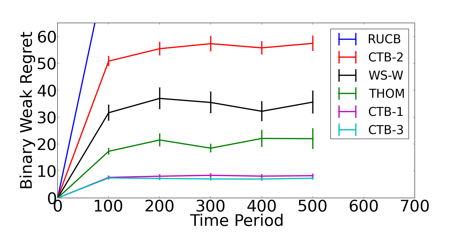
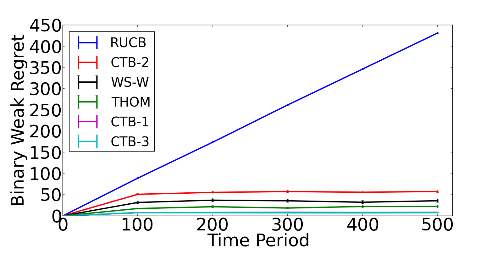
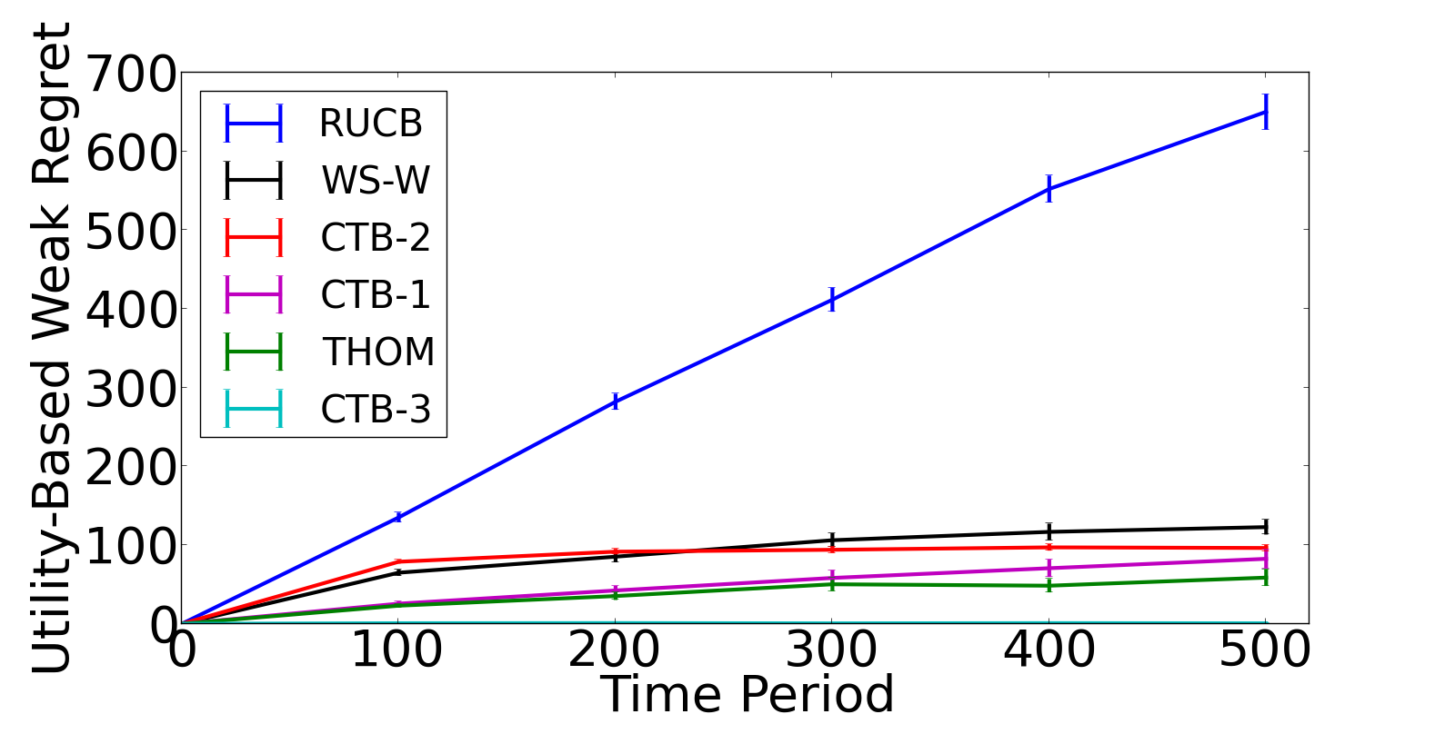
Since RUCB performs poorly in both experiments compared with other algorithms, we set the $y$-axis to emphasize the relative performance of the other algorithms. We include a plot over a wider $y$-axis showing RUCB’s performance in the supplement.

References

- Abbasi-Yadkori et al. (2011) Yasin Abbasi-Yadkori, Dávid Pál, and Csaba Szepesvári. Improved algorithms for linear stochastic bandits. In Advances in Neural Information Processing Systems, pages 2312–2320, 2011.
- Ailon et al. (2014) Nir Ailon, Zohar Shay Karnin, and Thorsten Joachims. Reducing dueling bandits to cardinal bandits. In ICML, volume 32, pages 856–864, 2014.
- Chen and Frazier (2017) Bangrui Chen and Peter Frazier. Dueling bandits with weak regret. In Proceedings of the 34st International Conference on Machine Learning (ICML-17), 2017.
- Franses and Montgomery (2002) Philip Hans Franses and Alan L Montgomery. Econometric models in marketing, volume 16. Elsevier, 2002.
- Jamieson and Nowak (2011) Kevin G Jamieson and Robert Nowak. Active ranking using pairwise comparisons. In Advances in Neural Information Processing Systems, pages 2240–2248, 2011.
- Joachims et al. (2007) Thorsten Joachims, Laura Granka, Bing Pan, Helene Hembrooke, Filip Radlinski, and Geri Gay. Evaluating the accuracy of implicit feedback from clicks and query reformulations in web search. ACM Transactions on Information Systems (TOIS), 25(2):7, 2007.
- Komiyama et al. (2015) Junpei Komiyama, Junya Honda, Hisashi Kashima, and Hiroshi Nakagawa. Regret lower bound and optimal algorithm in dueling bandit problem. In COLT, pages 1141–1154, 2015.
- Radlinski et al. (2008) Filip Radlinski, Madhu Kurup, and Thorsten Joachims. How does clickthrough data reflect retrieval quality? In Proceedings of the 17th ACM conference on Information and knowledge management, pages 43–52. ACM, 2008.
- Revelt and Train (1998) David Revelt and Kenneth Train. Mixed logit with repeated choices: households’ choices of appliance efficiency level. Review of economics and statistics, 80(4):647–657, 1998.
- Rusmevichientong and Tsitsiklis (2010) Paat Rusmevichientong and John N Tsitsiklis. Linearly parameterized bandits. Mathematics of Operations Research, 35(2):395–411, 2010.
- Yue and Joachims (2009) Yisong Yue and Thorsten Joachims. Interactively optimizing information retrieval systems as a dueling bandits problem. In Proceedings of the 26th Annual International Conference on Machine Learning, pages 1201–1208. ACM, 2009.
- Yue and Joachims (2011) Yisong Yue and Thorsten Joachims. Beat the mean bandit. In Proceedings of the 28th International Conference on Machine Learning (ICML-11), pages 241–248, 2011.
- Yue et al. (2012) Yisong Yue, Josef Broder, Robert Kleinberg, and Thorsten Joachims. The k-armed dueling bandits problem. Journal of Computer and System Sciences, 78(5):1538–1556, 2012.
- Zoghi et al. (2014) Masrour Zoghi, Shimon Whiteson, Remi Munos, Maarten de Rijke, et al. Relative upper confidence bound for the k-armed dueling bandit problem. In JMLR Workshop and Conference Proceedings, number 32, pages 10–18. JMLR, 2014.
- Zoghi et al. (2015) Masrour Zoghi, Zohar S Karnin, Shimon Whiteson, and Maarten De Rijke. Copeland dueling bandits. In Advances in Neural Information Processing Systems, pages 307–315, 2015.