Enhancing the Performance and Robustness of the FEAST Eigensolver
Abstract
The FEAST algorithm is a subspace iteration method that uses a spectral projector as a rational filter in order to efficiently solve interior eigenvalue problems in parallel. Although the solutions from the FEAST algorithm converge rapidly in many cases, convergence can be slow in situations where the eigenvalues of a matrix are densely populated near the edges of the search interval of interest, which can be detrimental to parallel load balancing. This work introduces two methods that allow one to improve the convergence robustness of the FEAST algorithm in these situations without having to increase the amount of computation. Selected numerical examples are presented and discussed.
I Introduction
| (1) |
by finding the eigenvectors whose eigenvalues lie in some interval of the user’s choosing. In this paper we consider the Hermitian standard eigenvalue problem for simplicity (i.e. and ), but the FEAST algorithm can be extended straight-forwardly to the generalized and non-Hermitian eigenvalue problems as well [3].
FEAST belongs to the broader family of contour integration eigensolvers [4, 5, 6, 7], but it can also be accurately described as an optimal subspace iteration procedure. A conventional subspace iteration consists of multiplying a trial subspace by the matrix and then orthogonalizing it with the Rayleigh-Ritz procedure; this process is repeated iteratively until the subspace converges. The FEAST algorithm operates similarly, but rather than multiplying the trial subspace by , one instead multiplies the trial subspace by the spectral projector matrix . The matrix is given by the complex contour integral
| (2) |
where is a closed contour in the complex plain that exactly encloses the interval on the real axis. The function applied to a real number is a filter function that returns 1 when and 0 otherwise. As a result, the matrix is a spectral projector whose image is the subspace that is spanned by only the eigenvectors of whose eigenvalues lie in . Multiplication of a vector by projects it into that subspace, and in this way the FEAST algorithm finds only the eigenvectors whose eigenvalues lie in [2]. The algorithm is outlined in Appendix. The contour integral (2) has no general analytical expression, so in practice the multiplication of a matrix by is approximated by using some numerical integration quadrature rule
| (3) |
where is the number of quadrature points, and each term is found by using a linear system solver with the column vectors of the matrix as the right hand sides of the linear system. A variety of quadrature rules are possible; in this work we use Gauss quadrature.
The benefits of using FEAST over a traditional subspace iteration technique are twofold. The first benefit is that, by finding only the eigenvectors whose eigenvalues lie in a certain interval, eigenvalue problems can be solved in parallel by solving for the eigenvector/eigenvalue pairs in different intervals independently.
The second benefit has to do with the rate of convergence. In a subspace iteration algorithm operating on a subspace of dimension , the eigenvector with the largest eigenvalue magnitude converges at a rate of , where is the eigenvalue with the largest magnitude. For a typical subspace iteration this means that the rate of convergence depends strongly on the eigenspectrum of . By using FEAST, the rate of convergence becomes [2], where is now the eigenvalue with the largest value of , and is the eigenvalue with the largest value of .
The ratio can be made arbitrarily large by either increasing the accuracy of the quadrature rule (3) by increasing , or by increasing the size of the subspace ; the eigenpairs anywhere in the spectrum can thus be found rapidly. It is not uncommon to be able to achieve a convergence rate of with and a subspace size of , where is the exact number of eigenvalues that lie in the interval . Because of these remarkable convergence properties, as well as its robustness and its ability to exploit parallelism at multiple levels, the FEAST algorithm and associated software package (www.feast-solver.org) have been very well received by the HPC community. The FEAST algorithm is currently featured as the principle HPC eigenvalue solver in the Intel Math Kernel Library (MKL).
The convergence rate of FEAST is not entirely insensitive to the spectrum of , however. In situations where the eigenvalues of are packed many times more closely together immediately outside of than they are inside of , the rate of convergence can be very slow. This is illustrated in Figure 1. The top plots in Figure 1 illustrate the situation where the density of the eigenvalue spectrum is the same both inside and outside the interval , and the bottom plots in Figure 1 illustrate the situation where the density is much larger outside of the interval than it is inside of the interval . The error at each FEAST subspace iteration is plotted for several values of and , and the corresponding values of and are indicated with horizontal dotted lines in the plots on the left in order to illustrate the effects of these parameters on convergence for both the dense spectrum and the sparse spectrum.
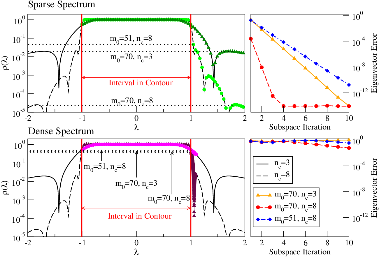
Even in situations that are less pathological than the one illustrated in the bottom plot of Figure 1, the varying density of the spectrum of can have negative implications for parallel load balancing. We can find the eigenpairs of in parallel by dividing the spectrum of into several non-intersecting intervals and then solving the eigenvalue problem for each interval separately and in parallel. When we do this, some intervals may converge more quickly than others due to the varying density of the spectrum, even if every interval contains the same number of eigenvalues. It is possible to speed up convergence in a given interval by increasing or , but this does not reduce the amount of computation required; increasing or increases the number of linear systems that need to be solved with each iteration, and the solution of the linear systems for the quadrature rule in equation (3) is where most of the computation in the FEAST algorithm occurs.
We would ideally like to be able to use parallel resources as efficiently as possible, performing the same amount of computation for each interval in which we solve the eigenvalue problem. We therefore would like to improve the convergence rate of FEAST in situations where the spectrum of results in slow or varying convergence rates, but without having to solve additional linear systems in order to do so.
In Ref. [8], this problem is addressed with the introduction of the Zolotarev quadrature that produces a very steep slope for the filter at the interval endpoints, which then leads to the same convergence rate between different contours. The Zolotarev approach presents, however, few limitations. The first limitation is that the convergence rate is fixed and cannot be improved while increasing , and it will thus underperform in comparison with Gauss quadrature, for example, in situations where the spectrum is sparsely packed or uniformely distributed (e.g. top plot of Figure 1); The second limitation is that the Zolotarev approach cannot be extended to the non-Hermitian problem where the eigenvalues are located in the complex plane.
In this work we propose a more general set of alternatives that use “accelerated subspace approach” strategies in order to improve the convergence robustness of FEAST regardless of which quadrature rule is being used.
II Accelerating the FEAST Subspace Iteration
Previous research [9] and the observation that larger subspace sizes increase the rate of convergence for FEAST suggest that we may be able to improve convergence by finding ways to increase the size of the subspace that is used in the Rayleigh-Ritz procedure. If we can do this without having to solve additional linear system right hand sides when performing the numerical quadrature in equation (3), then we may improve the convergence rate of FEAST without having to do too much additional computation. In the following subsections we discuss two ways of expanding the FEAST subspace size without solving additional linear systems.
II-A Method 1: Expand Subspace Using Previous Subspaces
In a typical FEAST subspace iteration, the trial subspace from the previous iteration is discarded and replaced with the filtered subspace (Step 1, FEAST Algorithm). Rather than discarding the previous subspace , we might instead append the new, filtered subspace to the old one before performing the Rayleigh-Ritz procedure; by doing this we can increase the dimension of the subspace by without having to solve additional linear systems. Step 1 of FEAST might then look like this:
- 1.
-
Filter the trial subspace and append it to the columns of the old one:
where we form by appending the column vectors of to the matrix for the previous subspace . We could repeat this process several times in order to build up a total subspace size of , after which we could keep the subspace size constant by removing old subspaces before adding new ones at each subspace iteration.
It would not be surprising if this modification of FEAST were to improve its the convergence rate; by expanding the subspace in this way, we are essentially building a Krylov subspace technique wherein we multiply our prospective subspace by powers of rather than by powers of .
If we modify step 1 of FEAST in this way then we have to make a few other modifications as well. Step 2(i) of FEAST requires the solution of the reduced eigenvalue problem , so we need to ensure that is symmetric positive definite; because we append the filtered subspace to the old one, this is no longer guaranteed. We therefore need to add another step to FEAST: orthogonalize the matrix before doing the Rayleigh-Ritz procedure. This can be done by using the QR decomposition or the singular value decomposition (SVD) of . For the research presented here, we orthogonalize by taking its SVD and setting equal to the left singular vectors:
| (4) |
In particular, we do this by diagonalizing
| (5) |
and then retaining the first columns of . Although this is less numerically stable than QR, we have found that it offers performance benefits in terms of the speed of the orthogonalization.
We call this algorithm ’expanding subspace FEAST’; see the XFEAST algorithm in Appendix.
The implementation of XFEAST we use in this paper also involves expanding the subspace to its full size before doing the first Rayleigh-Ritz procedure. The subspace size can be increased incrementally, with the Rayleigh-Ritz procedure being done in between each subspace expansion, but there is no reason to do this unless one expects that the algorithm might converge before the subspace size has reached its limit.
The part of step 2(ii) of XFEAST that specifies that one must select the desired eigenvectors is required because the subspace is expanded beyond just the filtered subspace. In conventional FEAST iterations the Rayleigh-Ritz procedure will find all of the eigenvectors whose eigenvalues are in the interval , plus the eigenvectors whose eigenvalues are closest to, but still outside of, . In XFEAST, because the subspace is expanded beyond the size , the Rayleigh-Ritz procedure will find all of those eigenpairs plus many more. Due to numerical errors it may even find eigenpairs for the Rayleigh-Ritz matrix that do not exist for the original matrix .
Since step 4(i) of XFEAST requires a subspace of dimension to filter with for the next iteration, we must select of the eigenpairs that are produced by step 2(i). Here, we are using a few steps of sorting. First, we calculate the error residuals for all eigenpairs from 2(i). We then select all of the eigenpairs whose eigenvalues lie inside the interval . If fewer than eigenpairs are found whose eigenvalues lie inside the contour interval, we then select additional eigenpairs from outside the contour as well, preferentially selecting those eigenpairs with the lowest residuals.
II-B Method 2: Expand Subspace Using Eigenvector Residuals
The other piece of information that the typical FEAST iteration generates (and which is otherwise discarded) is the eigenvector error residuals. Step 3 of the normal FEAST algorithm computes the eigenvector error residuals , and uses the one with the largest norm as a measure of the accuracy of the current subspace estimate.
Because the current eigenpair estimates provided at each iteration of FEAST come from the Rayleigh-Ritz procedure, the inner product of any of the estimated eigenvectors with any of the residual vectors is zero: . One can show this by using the fact that :
| (6) | ||||
If is the matrix of column vectors , then its column vectors span a subspace that is orthogonal to the current estimated solution subspace . We can therefore perform another Rayleigh-Ritz procedure in the subspace spanned by the combined columns of and without having to orthogonalize the column vectors of with respect to those of in order to ensure that is symmetric positive definite. This allows us to improve the estimated subspace without having to solve any additional linear systems and without having to do any orthogonalization procedure. A modified FEAST algorithm using this approach is given in the RFEAST algorithm in Appendix.
Again, it would not be surprising if adding eigenvector residuals to the subspace were to help improve the convergence rate; the eigenvalue algorithm LOBPCG [10] also works by including an eigenvector residual block in the search subspace.
Step 2(ii) of RFEAST again requires that we select the desired eigenpairs from amongst the ones produced by the Rayleigh-Ritz procedure. This is done in the same way as for XFEAST.
Measuring the error on the estimated subspace for RFEAST generally requires more care than in XFEAST or FEAST. The Rayleigh-Ritz procedure for RFEAST tends to produce many eigenpairs that do not exist in the spectrum of the full size matrix due to numerical error, and many of these spurious eigenpairs have eigenvalues that fall inside the interval .
In order to return the correct estimated eigenpairs and estimate the error on them, we must select only the eigenpairs inside that are not spurious. We do this by determining how many eigenpairs we should expect to find in that interval, and then taking that number of eigenpairs inside with the lowest residuals to be the eigenpairs of interest. We determine the number of eigenpairs to expect by counting the number of eigenpairs found during the first Rayleigh-Ritz procedure of each subspace iteration (i.e. during iteration in step 2 of RFEAST); the subspace used for the first Rayleigh-Ritz procedure is just the conventional FEAST subspace, and so we will not yet have produced the proliferation of spurious eigenpairs that comes from expanding the subspace by using the eigenvector residuals.
III Results and Comparisons
We demonstrate the convergence properties of these modified FEAST algorithms with several example matrices.
Figure 2 shows the eigenvector error residual at each subspace iteration of the FEAST, XFEAST, and RFEAST algorithms as applied to two different real symmetric matrices, for several different subspace sizes. Both matrices are dimension 545 and have the same eigenvectors, with 50 eigenvalues inside the FEAST interval [-1,1].
One matrix, labeled “Sparse” in Figure 2, has the other 495 eigenvalues in the interval [1.01, 20.81], whereas the one labeled “Dense” has those 495 eigenvalues in the interval [1.01, 1.1]. That is, the “Sparse” matrix has sparsely-packed eigenvalues outside of , and the “Dense” matrix has densely-packed eigenvalues outside of .
For the FEAST iterations the value of is the same as the subspace size, whereas for the XFEAST and RFEAST iterations is always set at 51, and the full subspace size is generated by one or the other subspace expansion method. XFEAST and RFEAST thus solve the same number of linear systems for each contour integration, regardless of the subspace size, whereas FEAST solves more linear systems for larger subspace sizes.
Despite solving many fewer linear system right hand sides per iteration (the number of linear system right hand sides per iteration is ), XFEAST and RFEAST outperform FEAST for the “Dense” matrix on a per-subspace iteration basis. This is not the case for the “Sparse” matrix. Nonetheless, even for the “Sparse” matrix, XFEAST and RFEAST do a similar amount of total computation for a given level of convergence.
FEAST Iterations for Sparse and Dense Eigenspectra

Figure 3 shows the amount of eigenvector error per number of linear system right hand sides solved for the same two matrices, for various values of and . The advantages of XFEAST and RFEAST are especially clear here; the rate of convergence per linear system right hand side solved, which is the majority of the computation in the FEAST algorithm, depends primarily on which algorithm is used in the case of the “Dense” matrix, with XFEAST and RFEAST clearly outperforming FEAST. XFEAST and RFEAST also outperform FEAST for the “Sparse” spectrum matrix, but here the difference is less dramatic.
Eigenvector Residual vs. # Linear RHS Solved

Figure 4 illustrates the results of solving an eigenvalue problem whose spectrum derives from electronic structure calculations [8, 11]. Our work here has been motivated by applications of this kind.
The left plot of Figure 4 shows the density of the eigenspectrum of the Hamiltonian matrix for the ground state of of a Caffeine molecule. The density of the eigenspectrum shows several distinct peaks, and one potential partitioning of the spectrum into two intervals is shown with red and blue lines. The right plot of Figure 4 shows the convergence trajectory when FEAST is used on each of these intervals separately. For the interval encompassed by Contour 2 (shown in red), the rightmost edge of which passes through a very dense region in the eigenspectrum, we also show the result of using XFEAST and RFEAST in order to try to achieve better convergence than is possible with FEAST.
The first interval (shown in blue), which has no eigenvalues immediately near its edges, converges rapidly, much like the second and third columns of the sparse example in Figure 2. The second interval, which has its upper limit passing through the middle of a dense group of eigenvalues, converges very slowly when using FEAST. This is the sort of problem that we seek to address.
FEAST Applied to Electronic Structure Spectrum

Using XFEAST and RFEAST, we can improve the final eigenvector error residual for the second, more challenging interval by more than four orders of magnitude. Still, this does not achieve ideal load balancing because the first interval has both of its edges in regions that are completely empty of eigenvalues, and so it converges very quickly. Better load balancing can only be achieved by dividing the spectrum in a less arbitrary way, which will require that we estimate the spectrum of a matrix before diagonalizing it. This is a subject of continuing research.
IV Conclusion
The results in Section III show that we can indeed improve the convergence rate of FEAST without solving additional linear systems by expanding the FEAST subspace through other means. This is particularly helpful in situations where the spectrum of the matrix at hand makes convergence difficult. Doing so comes at the price of having to use additional memory to store the expanded subspace; when using enough parallelism (and therefore a large enough number of intervals), however, we expect that memory will not be a constraint because the initial size of the subspace for each interval can be made almost arbitrarily small. As the results in Figure 4 show, though, this alone is not yet a fully satisfactory solution for achieving load balancing. Future work will consist of using this research to build on the efforts of others in order to estimate the eigenvalue distribution of a matrix [12] and efficiently divide the eigenvalue interval of interest [13]. We expect that, by combining our work here with these techniques for measuring and dividing and the eigenvalue spectrum of a matrix, we can achieve ideal load balancing in an automated way for arbitrary matrices.
Acknowledgments
The authors wish to acknowledge helpful discussions with Dr. Ping Tak Peter Tang and Dr. Yousef Saad. This material is supported by NSF under Grant #CCF-1510010.
References
- [1] E. Polizzi, “Density-matrix-based algorithm for solving eigenvalue problems,” Phys. Rev. B, vol. 79, p. 115112, 2009.
- [2] P. T. P. Tang and E. Polizzi, “Feast as subspace iteration accelerated by approximate spectral projection,” SIAM Journal on Matrix Analysis and Applications, vol. 35, p. 354–390, 2014.
- [3] J. Kestyn, E. Polizzi, and P. T. P. Tang, “FEAST Eigensolver for non-Hermitian Problems,” ArXiv e-prints 1506.04463, Jun. 2015.
- [4] T. Sakurai and H. Sugiura, “A projection method for generalized eigenvalue problems using numerical integration,” in Proceedings of the 6th Japan-China Joint Seminar on Numerical Mathematics (Tsukuba, 2002), vol. 159, no. 1, 2003, pp. 119–128.
- [5] T. Sakurai and H. Tadano, “CIRR: a Rayleigh-Ritz type method with contour integral for generalized eigenvalue problems,” Hokkaido Math. J., vol. 36, no. 4, pp. 745–757, 2007.
- [6] A. Imakura, L. Du, and T. Sakurai, “A block Arnoldi-type contour integral spectral projection method for solving generalized eigenvalue problems,” Appl. Math. Lett., vol. 32, pp. 22–27, 2014.
- [7] A. P. Austin and L. N. Trefethen, “Computing eigenvalues of real symmetric matrices with rational filters in real arithmetic,” SIAM J. Sci. Comput., vol. 37, no. 3, pp. A1365–A1387, 2015.
- [8] S. Güttel, E. Polizzi, P. T. P. Tang, and G. Viaud, “Zolotarev quadrature rules and load balancing for the feast eigensolver,” SIAM Journal on Scientific Computing, vol. 37, no. 4, pp. A2100–A2122, 2015.
- [9] B. Gavin and E. Polizzi, “Non-linear eigensolver-based alternative to traditional scf methods,” J. Chem. Phys., vol. 138, p. 194101, 2013.
- [10] A. V. Knyazev, “Toward the optimal preconditioned eigensolver: Locally optimal block preconditioned conjugate gradient method,” SIAM journal on scientific computing, vol. 23, no. 2, pp. 517–541, 2001.
- [11] A. R. Levin, D. Zhang, and E. Polizzi, “{FEAST} fundamental framework for electronic structure calculations: Reformulation and solution of the muffin-tin problem,” Computer Physics Communications, vol. 183, no. 11, pp. 2370 – 2375, 2012.
- [12] E. Di Napoli, E. Polizzi, and Y. Saad, “Efficient estimation of eigenvalue counts in an interval,” Numerical Linear Algebra with Applications, 2016, nla.2048.
- [13] S. Kajpust, “Variations of the feast eigenvalue algorithm,” Master’s thesis, Michigan Technological University, 2014.
FEAST Algorithm
Start with: Matrix to be diagonalized, interval wherein fewer than eigenvalues are expected to be found, initial guess for the subspace spanned by the solution to the eigenvalue problem .
- 1.
-
Filter the subspace to remove eigenvectors whose eigenvalues do not lie in the interval :
- 2.
-
Perform Rayleigh-Ritz procedure to find a new estimate for eigenvalues and eigenvectors:
- i.
-
Solve reduced eigenvalue problem , with and
- ii.
-
Get new estimate for subspace :
- 3.
-
Check the eigenvector error . If is above a given tolerance, GOTO 1.
XFEAST Algorithm
Start with: Matrix to be diagonalized, interval where fewer than eigenvalues are expected to be found, initial guess , and maximum number of subspaces to store .
- 0.
-
Repeatedly apply the filter procedure and append the resulting subspaces in order to expand the subspace to the predetermined size:
with .
- 1.
-
Orthogonalize the columns of
- 2.
-
Perform Rayleigh-Ritz procedure to find new estimate for eigenvalues and eigenvectors:
- i.
-
Solve reduced eigenvalue problem , with and
- ii.
-
Select the desired eigenpairs and get new estimate for :
- 3.
-
Check the eigenvector error . If is below a given tolerance, STOP.
- 4.
-
Update subspace:
- i.
-
Apply filter to new subspace estimate:
- ii.
-
Update subspace by removing the oldest subspace and appending the newest update:
- 5.
-
GOTO 1.
RFEAST Algorithm
Start with: Matrix to be diagonalized, interval where fewer than eigenvalues are expected to be found, initial guess , maximum number of Rayleigh-Ritz iterations .
- 1.
-
Filter the subspace to remove eigenvectors whose eigenvalues do not lie in the interval :
- 2.
-
Perform Rayleigh-Ritz procedure to find new estimate for eigenvalues and eigenvectors:
For to
- i.
-
Solve reduced eigenvalue problem , with and
- ii.
-
Select the desired eigenpairs and get new estimate for :
- iii.
-
Compute residual vectors and expand subspace:
end for
- 3.
-
Check the eigenvector error . If is above a given tolerance, GOTO 1.