Boosting the accuracy and speed of quantum Monte Carlo: size-consistency and time-step
Abstract
Diffusion Monte Carlo (DMC) simulations for fermions are becoming the standard for providing high quality reference data in systems that are too large to be investigated via quantum chemical approaches. DMC with the fixed-node approximation relies on modifications of the Green function to avoid singularities near the nodal surface of the trial wavefunction. Here we show that these modifications affect the DMC energies in a way that is not size-consistent, resulting in large time-step errors. Building on the modifications of Umrigar et al. and DePasquale et al. we propose a simple Green function modification that restores size-consistency to large values of the time-step, which substantially reduces time-step errors. The new algorithm also yields remarkable speedups of up to two orders of magnitude in the calculation of molecule-molecule binding energies and crystal cohesive energies, thus extending the horizons of what is possible with DMC.
The determination of accurate reference energetics for solids is one of the grand challenges of materials modelling. Reliable reference data is needed to make accurate predictions about any number of phenomena, such as phase stability, adsorption on surfaces and crystal polymorph prediction. Very often density functional theory (DFT) provides sufficient accuracy for this and as such has been immensely successful in furthering our understanding of materials [1, 2]. However, there are many materials and materials related problems for which DFT does not deliver the desired accuracy [3]. For such problems explicitly correlated wave-function based approaches are needed, such as the approaches of quantum chemistry, quantum Monte Carlo (QMC), and combinations thereof [4, 5, 6, 7, 8, 9, 10, 11, 12, 13, 14, 15]. In practice for condensed phase systems with more than a handful of atoms in the unit cell QMC remains the only feasible reference method, partly because of its favorable scaling with system size and the fact that it can be used efficiently on massively parallel supercomputers. Indeed QMC, mostly within the diffusion Monte Carlo (DMC) approach, is increasingly used to provide benchmark data for solids and to tackle interesting materials science problems that have been beyond the reach of DFT [16, 17, 18, 19, 20, 21, 22, 23, 24, 25, 26, 27, 28, 29]. DMC is also proving increasingly useful in exposing and helping to explain problems with DFT and as such in helping to further the development of DFT.
DMC is in principle an exact technique to solve the imaginary time dependent Schrödinger equation. The discretization of time in practical implementations introduces a time-step () error, the computational cost of which is proportional to . Recently Gillan et al. [21] showed that for CH4-H2O clusters current implementations of DMC appear to be non size-consistent, i.e. the total energy of a system of non-interacting molecules is not proportional to . Here we show that this is a general problem, we identify its source, and propose a simple modification that solves it. Moreover, we observe that the time-step error in binding energy evaluations is mostly due to this size-consistency issue. Our proposed method also leads to remarkable speedups, by significantly increasing the accuracy of large DMC evaluations 11 1 We note that other QMC approaches, such as the variational Monte Carlo (VMC) or the lattice regularized diffusion Monte Carlo (LRDMC) [11] do not suffer from these problems. This has been shown in [12], where the effect of the cutoff in the local energy on the size-consistency issue was carefully considered also for the latter method. In this paper, however, we are concerned with the much more widely used DMC..
A review of DMC can be found elsewhere [4, 31], and is summarized in Appendix A. To understand the size-consistency issue we recall the main ideas of the method and how it is applied in practice. Consider the Schrödinger equation in imaginary time for a system including particles with the fixed-node constraint, i.e. with the solution , where is the electronic configuration and the time, forced to have the same nodal surface of some guiding function (the hyper-surface where ). This is achieved, within the importance sampling scheme, by introducing the mixed distribution , which satisfies the equation:
| (1) |
Here we have omitted the functional dependence of the terms and is usually called the drift velocity, is the branching term, is the local energy, and is an energy shift. The three terms on the right hand side of Eq. 1 are responsible for diffusion, drift and branching processes, respectively. Eq. 1 can be rewritten in integral form:
| (2) |
where is the Green function for the importance sampling. The DMC method is a stochastic realization of Eq. 15, in which a series of walkers initially distributed as some is propagated ahead in time through a branching-drift-diffusion process, see Appendix A. In the limit the walkers end up distributed as , with the ground state of the Hamiltonian subject to the fixed-node constraint.
A practical implementation of Eq. 15 faces a problem: and diverge at the nodes of as the inverse of the distance between the nodal surface and . As these two singularities are not an issue because the drift term prevents the walkers from approaching the nodal surface. However, for finite , walkers can end up close to the nodal surface with catastrophic consequences. A practical solution to this problem is to introduce limits to the drift velocity and to the local energy. Umrigar, Nightingale and Runge [31] (UNR) proposed to replace with , defined as:
| (3) |
with an adjustable parameter between 0 and 1. This expression provides a rough approximation to the average velocity over a time-step, which has the effect of limiting the drift distance [31]. The branching factor is replaced with:
| (4) |
where is the best estimate of the energy, and . This limiting procedure is elegant and minimises instabilities because the divergences of at the nodes are cancelled by divergences in . As a result it is now standard in most DMC simulations. However, this limiting procedure is an approximation of the Green function which renders DMC size-inconsistent, see discussion in Appendix A.4.
The issue disappears for , where , but for the total energy is not proportional to the size of the system. Since the main application area of DMC is the calculation of medium to large systems for which relatively small energy differences are computed but very small cannot be afforded, this issue threatens the usefulness of DMC in material science.
To quantify the size-consistency problem consider two systems and with energies and , and define as the energy of the system with and at large enough distance from each other to have zero interaction. The quantity is therefore expected to be equal to zero and if it is not it measures the size-consistency error. To compute the binding energy of the system where and are interacting and have a total energy it is useful to define and . Here may be affected by a size-consistency problem, whereas is not. To illustrate the problem we have selected three representative examples with a broad range of interaction strengths, involving both isolated and periodic systems.
DMC simulations were carried out with the casino code [32]. We used Dirac-Fock pseudopotentials [33, 34] with the locality approximation [35]. The trial wavefunctions were of the Slater-Jastrow type with single Slater determinants and the single particle orbitals obtained from DFT-LDA plane-wave calculations performed with pwscf [36] and re-expanded in terms of B-splines [37].
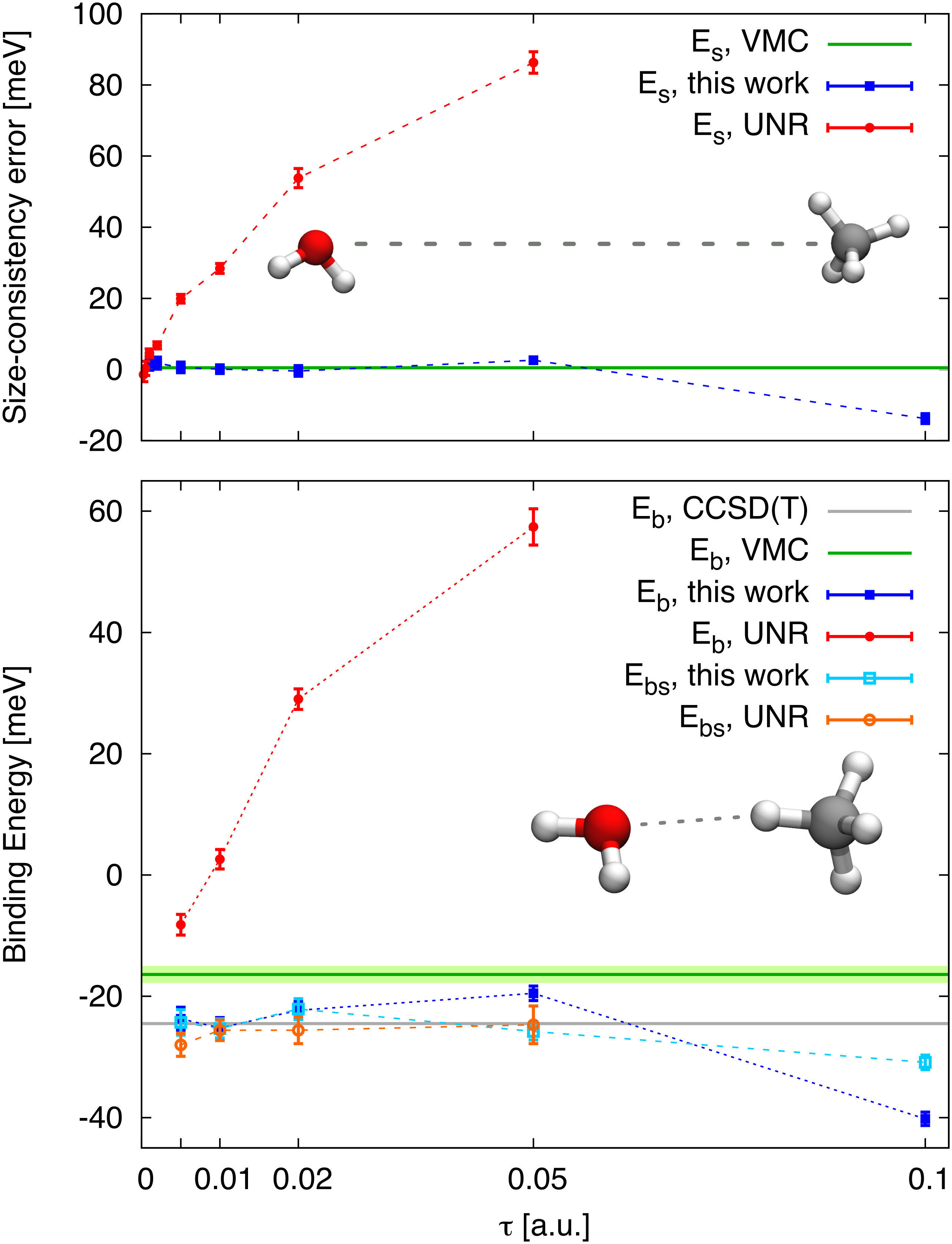
Our first example is a system formed by a CH4 () and a H2O () molecule. is obtained for a C-O distance of 11.44 Å. On the basis of CCSD(T) calculations we know that the residual interaction energy is meV, negligible for our purposes. is zero also for variational Monte Carlo (VMC), showing that the trial wavefunction of the dimer is effectively factorized: .
In Fig. 1 (top) we plot computed with DMC as a function of . For , as expected. However, at a typical time-step a.u. [21] the error is already 20 meV, which is about the same size as the binding energy of the dimer near the equilibrium distance, and it grows to over 80 meV at a.u.. In Fig. 1 (bottom) we show the binding energy of the molecule for a configuration near the equilibrium distance 22 2 Note that this is not the water-methane dimer equilibrium configuration, but just a configuration in which the C-O distance is near the equilibrium value. . As expected from the large size-consistency problem highlighted above, the binding energy computed with is wrong, and has a strong time-step dependence. Extrapolating to zero time-step using the whole range yields meV. Using only the range a value of meV is obtained, which is close to the benchmark energy meV, obtained with coupled cluster with singles, doubles and perturbative triples (CCSD(T) and a large basis set) [21]. By contrast, is effectively time-step independent up to , is in better agreement with the reference value, and removes the need for uncertain and arbitrary extrapolations. The UNR limiting procedure is too unstable above and even at we have not been able to obtain a very small statistical error due to instabilities in the simulation, see Appendix A.3.
Although one could envisage always using definitions analogous to to compute binding energies, it is much more desirable to be able to use instead, particularly when one is concerned with the binding energy of more than just a dimer 33 3 For example, in the case of a cluster formed by a large number of molecules the construction of the system with all molecules far enough away from each other could be difficult, or even impossible, and alternative correction schemes would be required [21]. .
To address this size-consistency issue we propose a new limiting procedure. As proven in Appendix A.4, the UNR limit for the drift term, Eq. 3, does not affect size-consistency, thus we only need to modify the branching term. Our method is based on the idea that any modifications to the Green function should be as insensitive as possible to the size of the system. Inspired by the prescriptions of DePasquale et al. [40], in which the local energy entering the branching factor is limited by a cutoff , a modified branching factor is defined as:
| (5) |
In the original [40] recipe . This has the consequence that for larger systems a larger fraction of the distribution of the branching factor is modified, leading again to a size-consistency issue. Here we propose:
| (6) |
where is the number of electrons in the system. Since the variance of the system is proportional to , this ensures that the proportion of the distribution of the branching factor modified by the cutoff is similar for systems with different values of 44 4 Note that, given the distribution of the branching factor of some system , the distribution of a system containing non-interacting copies of does not have, in general, the same form. This is because the central limit theorem implies that becomes Gaussian for large enough , but in general is not Gaussian. Thus the distribution cannot bemodified in a way that is exactly size-consistent and our proposed method is therefore only approximate.. As with the original approach [40], the exact Green function is restored in the limit . The parameter is an arbitrary constant to be conveniently chosen. For large enough values of (and/or small values of ) the Green function becomes exact, but then singularities reappear. For small values of (and/or large values of ) the bias in the DMC energy becomes large. We have found that a good compromise is obtained by setting . The results obtained with this newly proposed scheme are displayed in Fig. 1, showing that the bias in the DMC energy is now size-consistent up to very large values of . The new scheme also reduces the time-step error on the absolute energies, see Appendix B.
If the composite system is made of non-identical subsystems (like our water-methane system) then the method becomes less accurate at large , mainly because of the different widths of the distributions. In particular, the cutoff at a.u. corresponds to of around , and for CH4, H2O and CH4-H2O, respectively, where indicates the corresponding standard deviation of the VMC local energy 55 5 The standard deviation of the DMC distributions will, in general, be different from the of the VMC distributions, but the same arguments would apply. . With such small cutoff energies, the percentage of the respective distributions that are cut are different enough to affect the bias of the local energy in a non size-consistent way, which is why the error reappears at large values of .
Binding energies computed with the new method are displayed in the bottom panel of Fig. 1, showing that has the same accuracy as that computed with the UNR branching factor, but now also is accurate. The new method is stable also for 0.1 a.u., although at this very large value of the time-step the binding energy starts to show non negligible errors. Note that in order to obtain a sufficiently high accuracy on with the UNR branching factor, without relying on extrapolations, we would need to reduce the time-step to at least a.u., which is two orders of magnitude smaller than what is required with our newly proposed method.
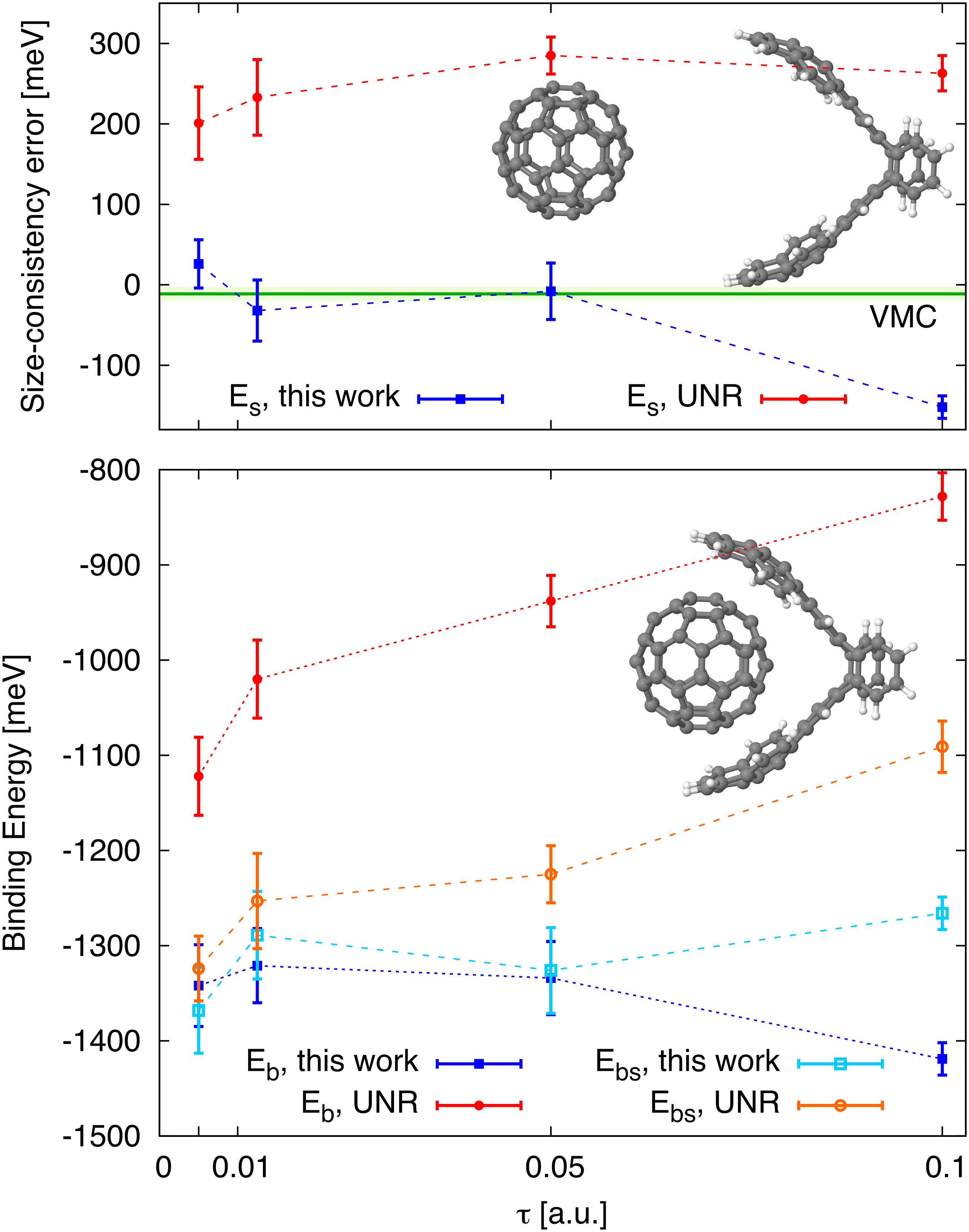
The second system we examined is the buckyball catcher, the C60-C60H28 () complex. This is an example of a whole class of supramolecular systems which is generally out of reach of the most accurate quantum chemistry methods and so at present DMC is the prime candidate for examining such systems. For the calculation of we considered the system with the two fragments separated by 10 Å. The residual interaction energy at this distance is meV [43], which is again negligible compared to the energies involved. The new limiting procedure results in very good cancellation of time-step error and it is size-consistent up to at least a.u.. The UNR branching factor causes a slightly larger time-step dependence of both and , and the top panel of Fig. 2 highlights once again the size-consistency problem. Incidentally, the binding energy of this complex reported in [44] was computed using UNR and , therefore it had a size-consistency error of 0.2 eV. Note that in this case any sensible extrapolation to zero time-step would result in a large size-consistency error, and therefore to obtain accurate results we should use a.u., if not even smaller, which is over two orders of magnitude more expensive and out of reach even on the biggest supercomputers currently available.
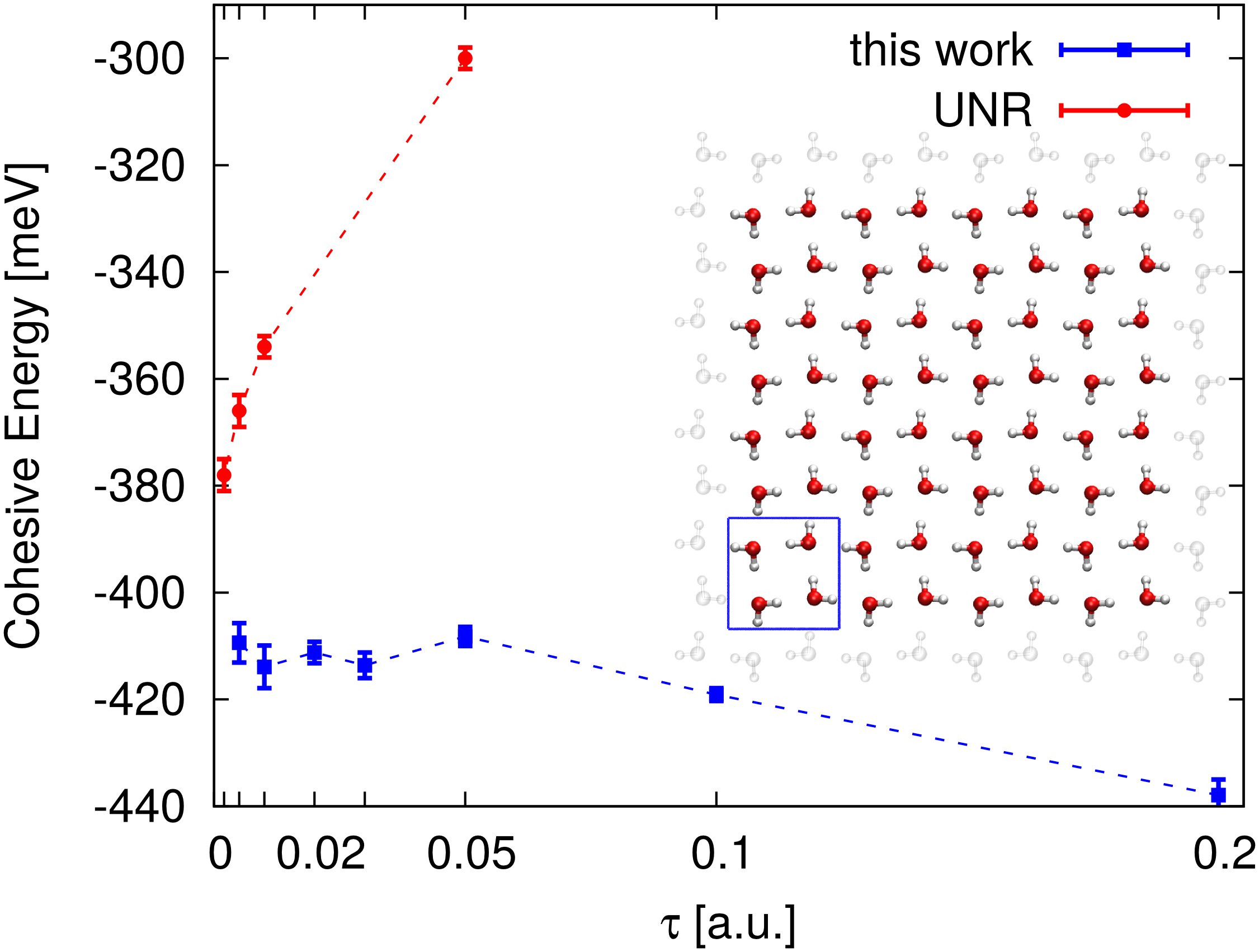
Our third and final test was performed on a square lattice ice system, a H-bonded 2D-periodic system which has been the subject of recent theoretical [45, 46] and experimental [47] studies. The simulation cell comprises 64 water molecules. In Fig. 7 we show the cohesive energy as a function of time-step. The cohesive energy computed with the new limiting procedure is independent of time-step up to at least a.u., while that computed with the UNR branching factor has errors even at the shortest time-step that we could afford ( a.u.). The non-linear trend of the UNR curve makes any extrapolation unreliable, unless simulations with a.u. could be afforded. Given the size of this system this makes such calculations prohibitively expensive. Remarkably, the new method does not require any uncertain time-step extrapolations and yields a speedup of around two orders of magnitude.
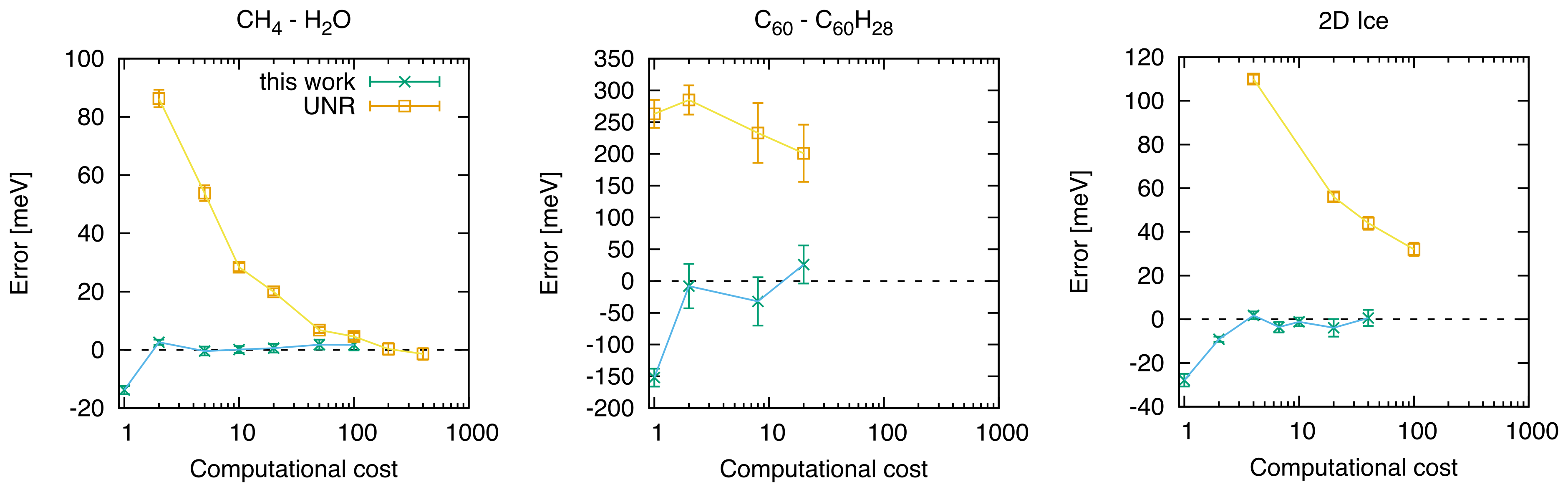
In summary, we have proposed a procedure that reduces DMC time-step errors by a large factor, and restores size-consistency. The method is based on the UMR scheme with an alternative branching factor. The modification is straightforward to implement, requiring just a change to a single line of code. We have demonstrated the new method on a CH4-H2O dimer, the C60-C60H28 supramolecular system and 2-dimensional ice. Besides solving the size-consistency problem, speedups of two orders of magnitude are obtained (see Fig. 4) and the need for time-step extrapolations is removed. The improvement appears particularly promising for investigations on molecular materials and to discriminate between crystal polymorphs. Moreover, the recent emergence of QMC-based molecular dynamics [24, 25, 26], which until now has only been affordable within VMC, could now be in reach with the more accurate fixed-node DMC approach.
Acknowledgements.
AZ and AM’s work has been sponsored by the Air Force Office of Scientific Research, Air Force Material Command, USAF, under grant number FA8655-12-1-2099 and by the European Research Council under the European Union’s Seventh Framework Programme (FP/2007-2013)/ERC Grant Agreement No. 616121 (HeteroIce project). AM is also supported by the Royal Society through a Wolfson Research merit Award. SS acknowledges CINECA for the use of computational facilities, under IscrB_SUMCHAL grant. Calculations were performed on the U.K. national service ARCHER, the UK’s national high-performance computing service, which is funded by the Office of Science and Technology through EPSRC’s High End Computing Programme. This research also used resources of the Oak Ridge Leadership Computing Facility located in the Oak Ridge National Laboratory, which is supported by the Office of Science of the Department of Energy under Contract No. DE-AC05-00OR22725. We thank Cyrus Umrigar for useful discussions and Jan Hermann for providing the estimated residual binding energy of the complex.Appendix
In the first section of Appendix A we provide a short review of the DMC method, followed by a description of the DMC algorithm, the problem of the divergences in proximity of the nodal surface, the instabilities in DMC simulations and the size-consistency issue met when DMC is stabilized by slightly modifying the algorithm. All this is used to contextualize the methodological improvements of this work. Appendices B, C and D provide further details on the three examples shown in the paper.
Appendix A Review of DMC
DMC energy evaluations are mostly concerned with the mixed estimator, defined as:
| (7) |
where is the guiding function (a parametrized wave function optimized within VMC schemes in order to be as close as possible to the ground state) and is the exact ground state wave function of the Hamiltonian . As long as has a non-zero overlap with , is equivalent to the pure estimator .
The exact wave function can be obtained from the solution of the imaginary time Schrödinger equation
| (8) |
where is the time, specifies the coordinates of the electrons, is the potential energy and is an energy offset. Given the boundary condition , for time the imaginary time solution converges to the ground state:
It is often convenient to write the time evolution of in terms of the Green function :
| (9) |
The Green function , which satisfies an equation analogous to that of , prescribes how to propagate further in time the distribution . Formally, we can write:
| (10) |
Unfortunately, is not exactly known for realistic systems. However, by considering that the time interval can be divided in smaller intervals of time , and iteratively using Eq. 9 to write in terms of , with and , we obtain the following expression for the Green function:
| (11) |
For a small enough time step , the Green function can be approximated using the Trotter-Suzuki formula, which results in:
| (12) |
where
is a diffusion term, and
is a branching term. The DMC algorithm is a stochastic realization of Eq. 9, in which a series of walkers initially distributed as some is propagated ahead in time with the short time approximation to the Green function in Eq. 12. In the long time limit the walkers become distributed as .
The method works perfectly well for bosons, as the ground state of the Hamiltonian is node-less. However, the fermionic ground state is generally difficult to calculate, because it is an excited state of the Hamiltonian. The difficulty comes from the fact that in the time evolution of Eq. 8 the weight of the ground state becomes exponentially dominant compared to excited states, and so the fermionic signal is quickly lost into noise. The common solution is to embrace the fixed node approximation: in constrained to have the same nodal surface of some guiding function . The constraint makes DMC only approximate, and the variational principle then implies that the fixed-node DMC energy is an upper bound of the true fermionic ground state energy. If the nodal surface of the guiding function is exact then also the fixed-node DMC energy is exact.
The fixed-node constraint is conveniently implemented by introducing the mixed distribution , which satisfies the equation:
| (13) |
(see Eq. 1), where is the drift velocity, or local gradient, and is the branching term, with the local energy. Note that in Eq. 13 there is an additional drift term that was not present in the original imaginary time Schrödinger equation for . The mixed distribution has the border condition and, in the limit of large time :
Thus, the mixed estimator can be written as:
| (14) |
It is convenient to write the time evolution of in terms of the Green function , which prescribes how to propagate further in time the distribution :
| (15) |
where satisfies an equation analogous to that of , and formally can be written as:
| (16) |
Again, is not exactly known for realistic systems, but we can use the same trick of splitting in time steps of length . We obtain the following expression for the Green function:
| (17) |
For a small enough time step , is approximated by the Green functions for purely drift, diffusion and branching processes. This leads to:
| (18) |
where
is the drift-diffusion term, and
is the branching term.
Eq. 13 also introduces importance sampling. Beside concentrating the sampling in the important part of the phase space, an additional advantage of importance sampling over simple sampling is that the branching term depends on the local energy , and not on the potential energy . Since is much smother than , and it is constant in the limit of , the stability of the DMC simulation is greatly enhanced. The error on this approximate expression for can be evaluated using the Zassenhaus formula [48], and the leading correction is of order . This translates into an error of order on (see Eq. 17). In the limit of the error on the Green function is zero, but the computational cost is because is split in terms.
A.1 DMC algorithm
We discuss here how the DMC algorithm actually works. At each time the distribution can be represented by a discrete set of walkers (i.e. sampling points with a weight ), such that . By using the Metropolis algorithm we can easily generate an ensemble of configurations (i.e., a set of walkers with unit weight) that correspond to the initial distribution . In DMC we need to project forward in time the walkers in order to calculated the mixed distribution for .
If in Eq. 14 we express the mixed distribution as in Eq. 15 (with initial distribution ), and we expand the Green function as in Eq. 17 (with ), we obtain that the mixed estimator is rewritten in the following way:
| (19) |
and using the approximation in Eq. 18 for the Green function with small we have:
| (20) |
Thus, according to the RHS of Eq. 20, each walker evolves in time according to a branching-drift-diffusion process: given the configuration and weight at time , the walker drift-diffuse as follows:
| (21) |
where is a -dimensional random vector generated from a normal distribution with zero mean and unit variance, and the walker weight evolves as:
| (22) |
The evolution of the weight is efficiently realized by using a branching (birth/death) algorithm, where walkers with small weight are killed and walkers with high weight are replicated [4]. Moreover, a Metropolis acceptance/rejection move is usually introduced after the drift-diffusion step[49, 31], in order to satisfy the detailed balance and reduce the time-step error, and with that an efficient time-step , which rescales the nominal time-step taking into account the acceptance probability, is used in Eq. 22 in place of .
Finally, given the chosen time-step and a sufficiently large number of DMC steps, the mixed energy is calculated as:
| (23) |
where is the average over all the walkers. Clearly, this evaluation is affected by a stochastic error inversely proportional to the square root of the number of walkers. In order to increase the precision of the evaluations it is not necessary to use a huge number of walkers; it is much more efficient, because of the equilibration time, to propagate further in time the walkers and to use the following expression to evaluate the mixed energy:
| (24) |
Notice that in Eq. 24 the walkers provide almost independent evaluations, but the local energies are instead serially correlated, with a correlation time proportional to . Thus, in evaluating the stochastic error for the mixed energy it is important to get rid of the serial correlation, for instance by using the “blocking method” [50]. Sometimes the estimator actually used can be slightly different from Eq. 24 – for instance some corrections are sometimes introduced in order to correct for the finite population bias (i.e., having a finite number of walkers can introduce a bias) – but the size-consistency issue here addressed is unaffected by these corrections.
A.2 Divergences in proximity of the nodal surface
Close to the nodal surface of the guiding function the approximation in Eq. 18 is problematic, because a configuration at a distance from has both the local gradient and the local energy (and consequently the branching term ) diverging in modulus as , leading to instabilities and big finite time step errors. This problem has been tackled both by DePasquale et al. [40] and Umrigar et al. [31], who proposed modifications for and for for close to to eliminate these divergences. These modifications are strictly related to the size-inconsistency issue addressed in this work.
A.3 DMC instabilities
DMC instabilities are uncontrolled walker population fluctuations (i.e., weights experiencing huge changes in a single step , see Eq. 22), which jeopardize the DMC energy evaluations and makes the simulation unfeasible. They are mainly due to walkers reaching regions of diverging local energy (because of the pseudo-potential or proximity to the nodal surface), and in particular for the branching term leads to proliferation of walkers from just one problematic configuration. Instabilities are strictly related with time step : with small instabilities are usually under control, but as larger and larger values of are considered instabilities are more often observed. The reason is that the diffusion step is random and proportional to , see Eq. 21, and if the time-step is too large there is some chance to fall into the problematic regions, because the drift step is unable to keep electrons away for the divergences. A small enough allows the drift step to recover from a “bad” diffusion step. As a matter of fact, DMC simulations with no modifications to the drift and branching terms are stable only for tiny values of , making schemes as those proposed by DePasquale et al. [40] or Umrigar et al. [31] necessary in actual calculations, the latter being much more stable than the former. The new limiting scheme proposed in this work (which is the same of Umrigar et al. [31] for the drift, Eq. 3 of the letter, and the one in Eq. 5 of the letter for the branching) appears as effective as the limiting scheme of Umrigar et al. [31] (see Eqs. 3 and 4 of the letter), if not better, in keeping the DMC simulation stable.
A pragmatic way to recover from a diverging population count (population explosion) is to back-track the simulation to a region far from the instability, run the random number generator idle for a number of cycles, and resume the DMC simulation. Often this procedure sends the simulation to a different region of phase space, avoiding the instability. However, if the instabilities are too frequent, the simulation becomes impractical or even impossible. To highlight the improvement in the stability of the calculations using the new limiting procedure, consider for example the CH4 - H2O dimer in the bound configuration. Using the UNR limiting procedure and a.u. we encountered 32 population explosions in steps (population size: 20,480 walkers). No simulations were possible with any larger value of time step. By contrast, using the new limiting procedure we observed no instabilities in steps at a.u., and also no instabilities in steps at a.u..
A.4 Size-consistency in DMC
As discussed in the letter, a method is size-consistent if the energy of any system constituted by the two non-interacting subsystems and , is equal to the sum of the energies of individual subsystems. As in the letter, we assume here to deal with systems that are size-consistent when described with a single Slater determinant (so, also with a Jastrow correlated single Slater determinant). In this section we show that the fixed-node DMC with importance sampling (i.e., Eq. 23) is size-consistent for any , but if the modifications to the branching proposed by Umrigar et al. [31] are used DMC is size-consistent only in the limit of .
Clearly, any configuration of the systems is given by the configurations and of the subsystems and , because any electron in AB belongs either to the subsystem or to . Mathematically, this means that the vectorial space where the configurations live is the direct sum of the two vectorial spaces where and live, and we can write (with a little abuse of notation):
| (25) |
As discussed in the letter, the guiding wave function factorizes, i.e.:
| (26) |
whenever and are far away. From the properties of the hamiltonian operator it follows that the local energy is additive:
| (27) |
which proves that VMC is size-consistent. Moreover, considering that the drift velocity is the local gradient, it is easy to show that:
| (28) |
where the symbol is used in the same way as in Eq. 25.
In order to address the properties of the DMC mixed energy evaluated for a finite value of the time-step, we can consider Eq. 23. According to Eq. 22, the weight is (here, for simplicity, we have slightly simplified the expression, neglecting that the first and last step have a weight that is 1/2) and including that the branching term , it is straightforward to see that:
| (29) |
By using Eq. 29, the additivity of the local energy (Eq. 27) and of the drift velocity (Eq. 28), and some algebra, it is easy to prove that:
| (30) |
for any value of the time-step , and of course also for . The main point of the proof is that the additivity of the local energy imply the factorization of the weight, i.e.:
| (31) |
In principle, it could be explicitly tested that DMC with no modifications satisfy the size-consistency for any finite time-step, but in practice it can be done only for very small values of because of the instabilities discussed in Section A.3.
The UNR modification to the drift, as reported in Eq. 3 of the letter, does not affect the additivity of the drift (because the correction is performed independently for each electron), and we have that:
| (32) |
which clearly does not affect the size-consistency of the method. The source of the size-inconsistency is instead the UNR modification to the branching term, see Eq. 4 in the letter, because we have that:
| (33) |
because of the term appearing in the expression of . This imply that the weight of a DMC realization does not factorize any more, that is:
| (34) |
However, in the limit of we have that and , thus UNR approaches asymptotically the case of no modifications, where size-consistency is proven.
The scheme proposed in this work (named here ZSGMA, from authors’ names), see Eqs. 5 and 6 in the letter, is exactly size-consistent for (namely, for or ), because the branching becomes equivalent to , which factorizes exactly, so we recover the unmodified DMC algorithm. The method is only approximated for finite ; the modified branching term is not exactly additive, i.e. , but what we approximatively satisfy is that:
| (35) |
at least when is large enough. This happens because, assuming that is properly set, we have that can be seen as a random variable of zero mean and a variance proportional to . In order to satisfy Eq. 35, at least approximatively, we require that the number of times we perform a cut on is independent on the size of the system and with a random sign. This implyes a value of .
Appendix B Water-Methane dimer
In Fig. 5 we display the energy of the dimer, as well and the energies of the monomers, and , computed in independent calculations performed with simulation cells containing either the CH4-H2O(shifted) dimer or the isolated CH4 and H2O monomers, respectively.
Single particle wavefunctions were obtained using a plane-wave cutoff of 300 Ry, and re-expanded in terms of B-splines with the natural grid spacing , where is the magnitude of the largest plane wave in the expansion. The Jastrow factor used in the trial wavefunction of the system included a two-body electron-electron (e-e) term; three different two-body electron-nucleus (e-n) terms for C, O and H, respectively; and three different three-body electron-electron-nucleus (e-e-n) terms, for C, O and H. Of course, for the isolated CH4 and H2O systems we only included the e-n and the e-e-n terms for C, H and O, H, respectively, but a part form this difference the Jastrow factors were exactly the same in all systems. The cutoff radii of the e-e, e-n, and e-e-n terms were all lower than 3.5 Å, and the large distance between the two molecules guarantees that the overlap between their respective orbitals is effectively zero. Therefore the trial wavefunction of the dimer , is effectively the appropriately antisymmetrised product of the trial wavefunctions and of the CH4 and the H2O sub-systems, respectively: . The variances of the local energy with the variational Monte Carlo (VMC) distributions were and Ha2 for the CH4-H2O, CH4 and H2O systems, respectively.
As seen in the paper, the finite time-step error in the binding energy, whenever the evaluation is used, is mostly due to the size consistency error. The speedup obtained by using present work prescriptions for the branching factor in comparison with UNR branching factor is of two orders of magnitude, as it is shown in Fig. 4(left). In this system there is the possibility to use and to alleviate the size-consistency issue of the UNR prescription for the branching factror. However, when big clusters or molecular crystals are considered, could be an unfeasible choice.
Appendix C The C60-C60H28 complex
As for the water-methane dimer, single particle wavefunctions were obtained using a plane-wave cutoff of 300 Ry, and re-expanded in terms of B-splines with the natural grid spacing . The Jastrow factor (e-e), (e-n) and (e-e-n) terms, and was constructed with the same procedure as in the water-methane system, i.e. by ensuring that it is the same in all systems. The variances of the VMC local energies were and Ha2 for the C60-C60H28, C60 and C60H28 systems, respectively.

In Fig. 6 we display the energy of the supramolecular system, as well as the energies of the monomers, and , computed in independent calculations performed with simulation cells containing either the isolated C60 and C60H28 molecules, respectively.
The improved accuracy of present work prescriptions for the branching factor in comparison with the UNR branching factor can be appreciated in Fig. 4(center).
Appendix D Two dimensional square ice
We considered a monolayer of flat square ice of water, that is a system with 2-dimensional periodicity that is attaining considerable attention [45, 47]. The unit cell include four water molecules, and here we considered a supercell, for a total of 64 waters in the system. The cohesive energy is obtained by subtracting the energy of the relevant number of isolated water molecules. Single particle wavefunctions were obtained using a plane-wave cutoff of 600 Ry, and re-expanded in terms of B-splines with the natural grid spacing . The larger plane-wave cutoff used for these calculations resulted in a lower variance of the VMC local energies, which was Ha2 for the isolated molecule, and Ha2 for the square ice (corresponding to Ha2 per water molecule). At the VMC level of theory the evaluated cohesive energy is -0.108(4) eV, that is severely underestimated (by a factor 4) with respect to the DMC evaluations.

In Fig. 7 we display the energy of the isolated water molecule, as well as the energy per water in the square lattice 2-dimensional system. A comparison with Fig. 5 shows that the higher quality of the trial wavefunctions for this system results in a lower time step error.
The speedup obtained with present work prescriptions for the branching factor in comparison with the UNR branching factor can be appreciated in Fig. 4(left).
References
- [1] J. Hafner, C. Wolverton, and G. Ceder, MRS Bulletin 31, 659 (2011).
- [2] J. Neugebauer and T. Hickel, Wiley Interdisciplinary Reviews: Computational Molecular Science 3, 438 (2013).
- [3] A. J. Cohen, P. Mori-Sanchez, and W. Yang, Chem. Rev. 112, 289 (2012).
- [4] W. M. C. Foulkes, L. Mitas, R. J. Needs, and G. Rajagopal, Rev. Mod. Phys. 73, 33 (2001).
- [5] C. Ochsenfeld, J. Kussmann, and D. S. Lambrecht, in Rev. Comput. Chem. (John Wiley & Sons, Inc., 2007) pp. 1–82.
- [6] R. Bartlett and M. Musiał, Rev. Mod. Phys. 79, 291 (2007).
- [7] G. K.-L. Chan and M. Head-Gordon, J. Chem. Phys. 116, 4462 (2002).
- [8] G. H. Booth, A. J. W. Thom, and A. Alavi, J. Chem. Phys. 131, 054106 (2009).
- [9] G. H. Booth, A. Grüneis, G. Kresse, and A. Alavi, Nature 493, 365 (2013).
- [10] S. Zhang and H. Krakauer, Phys. Rev. Lett. 90, 136401 (2003).
- [11] M. Casula, C. Filippi, and S. Sorella, Phys. Rev. Lett. 95, 100201 (2005).
- [12] M. Casula, S. Moroni, S. Sorella, and C. Filippi, J. Chem. Phys. 132, 154113 (2010).
- [13] J. Harl and G. Kresse, Phys. Rev. Lett. 103, 056401 (2009).
- [14] L. Schimka, J. Harl, A. Stroppa, A. Grüneis, M. Marsman, F. Mittendorfer, and G. Kresse, Nat. Mater. 9, 741 (2010).
- [15] X. Ren, P. Rinke, C. Joas, and M. Scheffler, J. Mater. Sci. 47, 7447 (2012).
- [16] B. Santra, J. Klimeš, D. Alfè, A. Tkatchenko, B. Slater, A. Michaelides, R. Car, and M. Scheffler, Phys. Rev. Lett. 107, 185701 (2011).
- [17] M. A. Morales, J. R. Gergely, J. McMinis, J. M. McMahon, J. Kim, and D. M. Ceperley, J. Chem. Theory Comput. 10, 2355 (2014a).
- [18] S. J. Cox, M. D. Towler, D. Alfè, and A. Michaelides, J. Chem. Phys. 140, 174703 (2014).
- [19] A. Benali, L. Shulenburger, N. A. Romero, J. Kim, and O. A. von Lilienfeld, J. Chem. Theory Comput. 10, 3417 (2014).
- [20] Y. S. Al-Hamdani, M. Ma, D. Alfè, O. A. von Lilienfeld, and A. Michaelides, J. Chem. Phys. 142, 181101 (2015).
- [21] M. J. Gillan, D. Alfè, and F. R. Manby, J. Chem. Phys. 143, 102812 (2015).
- [22] Y. Virgus, W. Purwanto, H. Krakauer, and S. Zhang, Phys. Rev. B 86, 241406 (2012).
- [23] M. Morales, R. Clay, C. Pierleoni, and D. Ceperley, Entropy 16, 287 (2014b).
- [24] G. Mazzola, S. Yunoki, and S. Sorella, Nat. Commun. 5, 3487 (2014).
- [25] G. Mazzola and S. Sorella, Phys. Rev. Lett. 114, 105701 (2015).
- [26] A. Zen, Y. Luo, G. Mazzola, L. Guidoni, and S. Sorella, J. Chem. Phys. 142, 144111 (2015).
- [27] J. Chen, X. Ren, X.-Z. Li, D. Alfè, and E. Wang, J. Chem. Phys. 141, 024501 (2014).
- [28] L. K. Wagner, Int. J. Quantum Chem. 114, 94 (2013).
- [29] L. K. Wagner and P. Abbamonte, Phys. Rev. B 90, 125129 (2014).
- [30] We note that other QMC approaches, such as the variational Monte Carlo (VMC) or the lattice regularized diffusion Monte Carlo (LRDMC) [11] do not suffer from these problems. This has been shown in [12], where the effect of the cutoff in the local energy on the size-consistency issue was carefully considered also for the latter method. In this paper, however, we are concerned with the much more widely used DMC.
- [31] C. J. Umrigar, M. P. Nightingale, and K. J. Runge, J. Chem. Phys. 99, 2865 (1993).
- [32] R. J. Needs, M. D. Towler, N. D. Drummond, and P. L. Rios, J. Phys.: Condens. Matter 22, 023201 (2010).
- [33] J. R. Trail and R. J. Needs, J. Chem. Phys. 122, 014112 (2005a).
- [34] J. R. Trail and R. J. Needs, J. Chem. Phys. 122, 174109 (2005b).
- [35] L. Mitas, E. L. Shirley, and D. M. Ceperley, J. Chem. Phys. 95, 3467 (1991).
- [36] S. Baroni, A. Dal Corso, S. de Gironcoli, and P. Giannozzi, http://www.pwscf.org.
- [37] D. Alfè and M. J. Gillan, Phys. Rev. B 70, 161101 (2004).
- [38] Note that this is not the water-methane dimer equilibrium configuration, but just a configuration in which the C-O distance is near the equilibrium value.
- [39] For example, in the case of a cluster formed by a large number of molecules the construction of the system with all molecules far enough away from each other could be difficult, or even impossible, and alternative correction schemes would be required [21].
- [40] M. F. DePasquale, S. M. Rothstein, and J. Vrbik, J. Chem. Phys. 89, 3629 (1988).
- [41] Note that, given the distribution of the branching factor of some system , the distribution of a system containing non-interacting copies of does not have, in general, the same form. This is because the central limit theorem implies that becomes Gaussian for large enough , but in general is not Gaussian. Thus the distribution cannot bemodified in a way that is exactly size-consistent and our proposed method is therefore only approximate.
- [42] The standard deviation of the DMC distributions will, in general, be different from the of the VMC distributions, but the same arguments would apply.
- [43] J. Hermann, Private communication.
- [44] A. Tkatchenko, D. Alfè, and K. S. Kim, J. Chem. Theory Comp. 8, 4317 (2012).
- [45] J. Chen, G. Schusteritsch, C. J. Pickard, C. G. Salzmann, and A. Michaelides, Phys. Rev. Lett. 116, 025501 (2016).
- [46] F. Corsetti, P. Matthews, and E. Artacho, Sci. Rep. 6, 18651 (2016).
- [47] G. Algara-Siller, O. Lehtinen, F. C. Wang, R. R. Nair, U. Kaiser, H. A. Wu, A. K. Geim, and I. V. Grigorieva, Nature 519, 443 (2015).
- [48] M. Suzuki, Commun. Math. Phys. 57, 193 (1977).
- [49] P. J. Reynolds, D. M. Ceperley, B. J. Alder, and W. A. Lester, J. Chem. Phys. 77, 5593 (1982).
- [50] H. Flyvbjerg and H. G. Petersen, J. Chem. Phys. 91, 461 (1989).