Planck intermediate results. XLIX. Parity-violation constraints from polarization data
Abstract
Parity violating extensions of the standard electromagnetic theory cause in vacuo rotation of the plane of polarization of propagating photons. This effect, also known as cosmic birefringence, impacts the cosmic microwave background (CMB) anisotropy angular power spectra, producing non-vanishing – and – correlations that are otherwise null when parity is a symmetry. Here we present new constraints on an isotropic rotation, parametrized by the angle , derived from Planck 2015 CMB polarization data. To increase the robustness of our analyses, we employ two complementary approaches, in harmonic space and in map space, the latter based on a peak stacking technique. The two approaches provide estimates for that are in agreement within statistical uncertainties and very stable against several consistency tests. Considering the – and – information jointly, we find from the harmonic analysis and from the stacking approach. These constraints are compatible with no parity violation and are dominated by the systematic uncertainty in the orientation of Planck’s polarization-sensitive bolometers.
Key Words.
cosmology: theory – observations – cosmic background radiation – polarization – methods: data analysis – methods: statistical1 Introduction
Measuring the in vacuo rotation of the plane of polarization of photons is a way to test fundamental physics in the Universe. Such a rotation is sensitive to parity-violating interactions in the electromagnetic sector that are found in extensions of the Standard Model of particle physics (Carroll 1998; Lue et al. 1999; Feng et al. 2005; Li et al. 2009). For example, extending the Maxwell Lagrangian with a coupling (scalar, Chern-Simons, etc.) to ,11 1 Here is the photon field, and is the dual of the Faraday tensor, defined to be . impacts right- and left-handed photons asymmetrically. Therefore a photon at the last-scattering surface with linear polarization in one orientation will arrive at our detectors with its plane of polarization rotated due to this coupling term. The amount of rotation, usually denoted , is often referred to as the cosmic birefringence angle. This rotation naturally mixes - and -modes of CMB polarization22 2 We use the customary convention used by the CMB community for the Q and U Stokes parameters, see e.g. http://wiki.cosmos.esa.int/planckpla2015/index.php/Sky_temperature_maps. and generates – and – correlations that would be zero in the absence of parity violations. The cosmic microwave background (CMB) polarization is particularly useful for measuring such an effect, because even if the coupling is small, CMB photons have travelled a large comoving distance from the last-scattering surface (almost) completely unimpeded and thus the rotation could accumulate into a measurable signal.
This effect has previously been investigated using data from many CMB experiments (Feng et al. 2006; Wu et al. 2009; Brown et al. 2009; Pagano et al. 2009; Komatsu et al. 2011; Hinshaw et al. 2013; Ade et al. 2014a; Ade et al. 2014b; Kaufman et al. 2014; Naess et al. 2014; di Serego Alighieri et al. 2014; Zhao et al. 2015; Mei et al. 2015; Gruppuso et al. 2015; Contaldi 2015; Molinari et al. 2016), and also by looking at radio galaxy data (Carroll et al. 1990; Cimatti et al. 1993; Cimatti et al. 1994; Wardle et al. 1997; Leahy 1997; Carroll 1998; di Serego Alighieri et al. 2010; Kamionkowski 2010). Thus far all the constraints are compatible with no cosmic birefringence (see discussion in Sect. 7).
In this paper we employ Planck33 3 Planck (http://www.esa.int/Planck) is a project of the European Space Agency (ESA) with instruments provided by two scientific consortia funded by ESA member states and led by Principal Investigators from France and Italy, telescope reflectors provided through a collaboration between ESA and a scientific consortium led and funded by Denmark, and additional contributions from NASA (USA). 2015 CMB data to estimate an isotropic . The birefringence angle has already been constrained with Planck data in Gruppuso et al. (2015), using the publicly available 2015 Planck Likelihood (Planck Collaboration XI 2016). However, that work did not use – and – data, which are essential for determining the sign of and for increasing the constraining power. We include here – and – cross-correlations by considering two approaches, one based on harmonic space, through the use of the so-called “-estimators” and one based on pixel-space maps that employs stacked images of the (transformed) and Stokes parameters.
The paper is organized as follows. In Sect. 2 we describe the effect that cosmological birefringence has on the angular power spectra of the CMB. In Sect. 3 we provide details of the data and simulations that are considered in our analysis, which is described in Sect. 4. Results for our two different methodologies are summarized and compared in Sect. 5. Section 6 contains a discussion of the systematic effects that are most important for the observables considered. Finally, conclusions are drawn in Sect. 7.
2 Impact of birefringence on the CMB polarization spectra
Birefringence rotates the six CMB angular power spectra in the following way (see Lue et al. 1999; Feng et al. 2006, for more details):
| (1) | ||||
| (2) | ||||
| (3) | ||||
| (4) | ||||
| (5) | ||||
| (6) |
Here is assumed to be constant (see Liu et al. 2006; Finelli & Galaverni 2009; Li & Zhang 2008 for generalizations). In this paper we will consider only the above parametrization, where the primed are the observed spectra and the unprimed are the spectra one would measure in the absence of parity violations. In principle the rotation angle could depend on direction (with details dictated by the specific model considered), and one could measure the anisotropies of . We do not employ this type of analysis here, but focus on the simple case of an isotropic (or the monopole) (see Gluscevic et al. 2012 and Ade et al. 2015 for constraints on anisotropic birefringence).
Isotropic birefringence is indistinguishable from a systematic, unknown mismatch of the global orientation of the polarimeters. This is strictly true if the cosmological birefringence is the same regardless of the multipole at which CMB polarization is measured. However, specific birefringence models may predict some angular dependence in . Furthermore, large angular scale polarization in is sourced in the re-ionization epoch, as opposed to the small scales which are formed at recombination (Komatsu et al. 2011; Gruppuso et al. 2015). This will inevitably produce some angular dependency in (assuming that the birefringence angle is proportional to the CMB photon path) and this effect could in principle be used to disentangle instrumental systematic effects (since photons that scattered at the re-ionization epoch would have traveled less than the others). However, we focus here on smaller scale data, where the reionization effects are not important and therefore such a distinction is not possible. For Planck there is an estimate of the uncertainty of the possible instrument polarization angle using measurements performed on the ground (Rosset et al. 2010), as discussed further in Sect. 6. Unfortunately, in-flight calibration is complicated by the scarcity of linearly polarized sources that are bright enough, with the Crab Nebula being a primary calibration source (Planck Collaboration VIII 2016).44 4 We do not employ any self-calibration procedure as suggested in Keating et al. (2012), since it is degenerate with the effect we are looking for.
Eqs. (1)–(6) include all the secondary anisotropies but the weak-lensing effect. Due the current precision of data (Gubitosi et al. 2014, see the discussion in) we safely ignore the weak-lensing effect as it contributes a negligible error.
3 Data and simulations
We use the full-mission Planck (Planck Collaboration I 2016) component-separated temperature and high-pass-filtered polarization maps at HEALPix55 5 http://healpix.sourceforge.net/ (Górski et al. 2005) resolution ; i.e., we take the Commander, NILC, SEVEM, and SMICA solutions for , , , and , fully described in Planck Collaboration IX (2016) and Planck Collaboration X (2016), and available on the Planck Legacy Archive.66 6 http://www.cosmos.esa.int/web/planck/pla The -mode maps are calculated using the method of Bielewicz et al. (2012, see also ). We use the common temperature and polarization masks at , namely UT102476 and UPB77, respectively. For the harmonic analysis we also use half-mission data provided by the SMICA component-separation pipeline, in order to build our -estimator from cross-correlations (Planck Collaboration IX 2016). No further smoothing is applied to any of the maps (although this version of the data already includes 10′ smoothing in both temperature and polarization).
We note that there are known systematic effects in the polarization maps released by Planck that have not been fully remedied in the 2015 release (see Sect. 6 for a full discussion on the main systematic effects relevant for this analysis). These issues include various sources of large angular scale artefacts, temperature-to-polarization leakage (Planck Collaboration VII 2016; Planck Collaboration VIII 2016; Planck Collaboration XI 2016), and a mismatch in noise properties between the data and simulations (Planck Collaboration XII 2016). In order to mitigate any large-angle artefacts, we use only the high-pass-filtered version of the polarization data. We note that neglecting the large scales has little to no impact on our constraining power for . We have also checked that temperature-to-polarization leakage (Planck Collaboration XI 2016) has very little effect on our analysis (see Sect. 6.2); similar conclusions are reached in Planck Collaboration XLVI (2016).
We pay particular attention to the mis-characterization of the noise in the polarization data. Given the recommendation in Planck Collaboration IX (2016) we restrict our analysis to cross-correlation and stacking methods, which are less sensitive to such noise issues (Planck Collaboration VIII 2016). For the harmonic analysis, we estimate the angular power spectra up to multipoles (Planck Collaboration IX 2016, as suggested by the cosmological analysis tests carried out in), using simulations to create a statistic. The map-space analysis does not require the use of simulations,77 7 We explicitly checked that using simulations does not change the results, which is simply a consequence of the fact that the process of stacking means we are not very sensitive to the noise properties of the data. since we only need a relatively crude noise estimate on the scales we work at and we use a weighting approach when stacking that is only dependent on the data (we have also checked that our results are quite insensitive to the noise level of the data, see Sect. 6.1). Nevertheless it is reassuring that the map-space and harmonic-space analyses arrive at consistent results.
We use realistic full focal plane (FFP8.1) simulations described in detail in Planck Collaboration XII (2016). These are simulations processed through the four Planck component-separation pipelines, namely Commander, NILC, SEVEM, and SMICA (Planck Collaboration IX 2016), using the same weights as derived from the Planck full mission data. The CMB output maps are used to build the harmonic space estimators used in this work. For our harmonic space estimator we use the half-mission simulations provided by the SMICA pipeline.
The FFP8.1 fiducial cosmology corresponds to the cosmological parameters , , , , , , , and (where ). Note that we perform the analysis for the birefringence angle by fixing the other cosmological parameters to the values reported above. This seems to be a safe assumption, since in Gruppuso et al. (2015) it was shown that is quite decoupled from the other parameters, at least as long as , , and are considered; CDM parameters are not expected to be constrainted much from and , contrary to models that explicitly break parity symmetry.
4 Analysis
4.1 Map-space analysis
We follow the stacking approach first introduced in Komatsu et al. (2011), where they were able to constrain by stacking polarization on temperature extrema. Here we perform the same analysis, but also stack on -mode extrema. Our analysis is performed in map space (although we must briefly go to harmonic space for stacking on -modes, as described in Sect. 6.1) and we show that stacking polarization on temperature extrema is sensitive to the – and – correlations, while stacking on -mode extrema is sensitive to the – and – correlations.
The recommendation on the use of polarization data from Planck Collaboration IX (2016) is that only results with weak dependence on noise are to be considered completely reliable. For the purposes of stacking on temperature peaks only cross-correlation information is used, and thus understanding the detailed noise properties of polarization is unnecessary. Stacking on -mode peaks the results do depend on the noise properties of the map; this is because the expected angular profiles of the stacks depend on the full power spectrum of the map. In Sect. 6.1 we demonstrate that even a strong miscalculation of the noise would result in shifts at below the level (and more reasonable miscalculations of the noise will bias results at an essentially negligible level).
4.1.1 and parameters
We use the transformed Stokes parameters , and , first introduced in Kamionkowski et al. (1997):
| (7) | ||||
| (8) |
Here is defined as the angle from a local “east” (where “north” always points towards the Galactic north pole) direction in the coordinate system defined by centring on the hot or cold spot, and is a radial vector. The stacking procedure tends to produce images with azimuthal symmetry, and hence the predictions will only depend on . The theoretical angular profiles for stacking on temperature hot spots are derived in Komatsu et al. (2011, see also ) and are explicitly given by
| (9) | ||||
| (10) |
The quantities are combinations of the beam (10′ smoothing) and pixel window functions (at ) for temperature and polarization. Below we will use to denote the same quantity for -modes; however, the -modes are produced at the same resolution as temperature and so . The bracketed term in each of Eqs. (9) and (10) incorporates the scale-dependent bias when converting the underlying density field to temperature or -modes (thus, they will differ if the stacking is performed on temperature or -mode extrema). The function is the second-order Bessel function of the first kind. Angular profiles derived from stacking on -mode hot spots can easily be generalized from the above formulae by simply noting that -modes share the same statistical properties as temperature and thus we only need to change the power spectra in the above formulae. Thus the angular profiles for stacking on -mode hot spots are given by
| (11) | ||||
| (12) |
The specific forms of (the scale-independent part) and (which is proportional to second derivatives that define the peak) are given in Desjacques (2008). The CDM prediction for is identically zero and thus we will find that the vast majority of the constraining power comes from these profiles. We also show explicitly in Eqs. (9)–(12) that and are sensitive to the – and – correlation when stacking on temperature extrema or the – and – correlation when stacking on -mode extrema. Determination of the bias parameters depends on the power spectrum of the map where the extrema are determined (see Komatsu et al. 2011, and Appendix A), thus they depend on the noise properties of the map, as well as the underlying power spectrum. Section 6.1 will examine to what extent misunderstanding the noise might bias the results.
For our main results we have selected extrema using a threshold of , which mean we consider all positive hot spots (or negative cold spots); however, we have checked other choices of threshold and found consistency, provided that we do not choose such a high a threshold such that the overall signal becomes too weak. We do not claim that our analysis is optimal, and it may be that a better weighting exists for different levels of threshold; however, tests have shown that, in terms of minimizing the uncertainty on , the choice of and use of averaged bias parameters is close to optimal.
For the Planck temperature data we calculate the bias parameters to be K-1 and K-1. For the Planck -mode data we calculate K-1 and K-1 for Commander, NILC, SEVEM, and SMICA, respectively. The derivation of Eqs. (9)–(10) and a discussion of how to calculate all relevant quantities are given in appendix B of Komatsu et al. (2011), while the derivation of Eqs. (11)–(12) is given in Appendix A of this paper. The reader is referred to Komatsu et al. (2011) and also section 8 of of Planck Collaboration XVI (2016) for a complete description of the physics behind the features in the predicted stacked profiles.
4.1.2 Procedure
We begin by locating all local extrema88 8 As previously mentioned, we use all positive (negative) local maxima (minima) for hot (cold) spots. Extrema are defined by comparing each pixel to its nearest neighbours. of the temperature (or -mode) data outside the region defined by the mask, i.e., either the union of temperature and polarization common masks for stacking on temperature extrema or simply the polarization common masks when stacking on -mode extrema. These masks remove the Galactic plane, as well as the brighter point sources. We define a 55∘ grid, with the size of each pixel being and the number of pixels being 2500. When adding and images, we weight each pixel by the number of unmasked pixels that lie in each re-gridded pixel (which is not uniform, because of the re-gridding and masking; this weighting is used in the estimation of the covariance matrix of the stacked images). Therefore the pixels near the centre generally have somewhat lower noise in the final stacked image. We then generate and images using Eqs. (7) and (8).
The predictions for and are found by combining Eqs. (9)–(12) with Eqs. (2)–(6):
| (13) | ||||
| (14) |
For stacking on -modes we have
| (15) | ||||
| (16) |
where we have assumed that , which is consistent with our data, since Planck does not have a direct detection of -modes. We use a uniform prior on , , when sampling the likelihood, i.e.,
| (17) |
with
| (18) |
Here represents the data, consisting of the stacked and images, and are the predictions as a function of (see Eqs. 13–16). The quantity is the covariance matrix, which is a combination of the noise in the data and the cosmic variance due to the limited number of hot (or cold) spots in the sky. We have estimated the covariance matrix by determining an rms level from the pixelization scheme chosen and then weighting this with the inverse of the total number of pixels used in each re-gridded pixel; we have also assumed that the covariance is diagonal in pixel space.
For the purposes of evaluating the likelihood, we have fixed and to the theoretical power spectra, based on the best-fit Planck parameters (Planck Collaboration XIII 2016), and simply evaluate the likelihood in a fine grid of values. The choice of fixing the angular power spectra is reasonable because the usual cosmological parameters are determined by and , which are minimally affected by (no dependence, quadratic, and still quadratic dependence on , respectively). See also comments at the end of Sect. 3.
Finally, we quote the mean of the posterior on and the width of the posterior containing 68 % of the likelihood as the best-fit and statistical uncertainty, respectively. The posterior for is sufficiently Gaussian that these two values contain all necessary information about the posterior.



4.2 Harmonic-space analysis
The harmonic-based analysis uses the so-called -estimators (Wu et al. 2009; Gruppuso et al. 2012; Zhao et al. 2015; Gruppuso et al. 2016, see for instance), which are defined by the following equations:
| (19) | |||||
| (20) |
Here is the estimate for the birefringence angle . It is possible to show that on average
| (21) | |||||
| (22) |
Eqs. (21) and (22) are zero when
| (23) |
Eq. (23) suggests that we can find by looking for the that makes null the expectation values of the -estimators. From now on we always consider that Eq. (23) is satisfied.
We estimate the angular power spectra using the MASTER method (Hivon et al. 2002) extended to polarization (Kogut et al. 2003; Polenta et al. 2005) to correct for masking, and we use simulations to estimate the noise. We choose a bin size of , starting at , to avoid correlations between bins induced by masking. It is then possible to minimize for and separately, or jointly to estimate :
| (24) |
where or , denotes the bin and , where the average is taken over the FFP8.1 simulations described in Sect. 3 and generated with . We thus are adopting a simple frequentist approach to test the null hypothesis of no parity violation. This approach also allows for the minimization of Eq. (24) in subintervals of multipoles, providing the possibility of searching for a possible angular scale dependence to the birefringence effect, i.e.,
| (25) |
where . This will be used to test the stability of the estimates of against the ranges of multipoles considered for the CMB spectra.
The -estimator is inherently built from cross-correlations (see Eq. 19) and therefore we are able to use the full-mission data and simulations for all component-separation methods to generate the corresponding . Moreover, since the SMICA simulations are also delivered in half-mission form, we are additionally able to estimate by cross-correlating half-mission 1 and half-mission 2 data and simulations.
Regarding the -estimator, since it contains auto-correlations (see Eq. 20), we must estimate it from the half-mission data along with simulations in order to satisfy the recommendations on the use of polarization data given in Planck Collaboration IX (2016), based on the fact that only results with a weak dependence on noise are to be considered fully reliable. More specifically, and are estimated from cross-correlating half-mission 1 with half-mission 2 SMICA data and using the corresponding SMICA simulations only.
5 Results
In the following subsections we present our constraints on for the two methods, described in the previous section. We will quote our best-fit values and uncertainties (statistical only, leaving consideration of systematic effects to Sect. 6). We will show specifically that the – correlation is more constraining than the – correlation. This is expected and can be demonstrated directly by computing the variance of Eqs. (5) and (6). For small , the variance of based on – and – information alone is
| (26) | ||||
| (27) |
respectively. This can be derived from the Fisher information matrix, where the covariance is a simple matrix containing the variance of – or –. Thus, as suggested by the above relations, our results based on – are generally more constraining than our – results (the presence of noise, however, will modify these relations).
With respect to statistical uncertainty, we will demonstrate that our results are robust to all component-separation methods, and with respect to our two methods. For convenience, we offer a direct comparison of results obtained by our two approaches in Fig. 7.
5.1 Map-space results
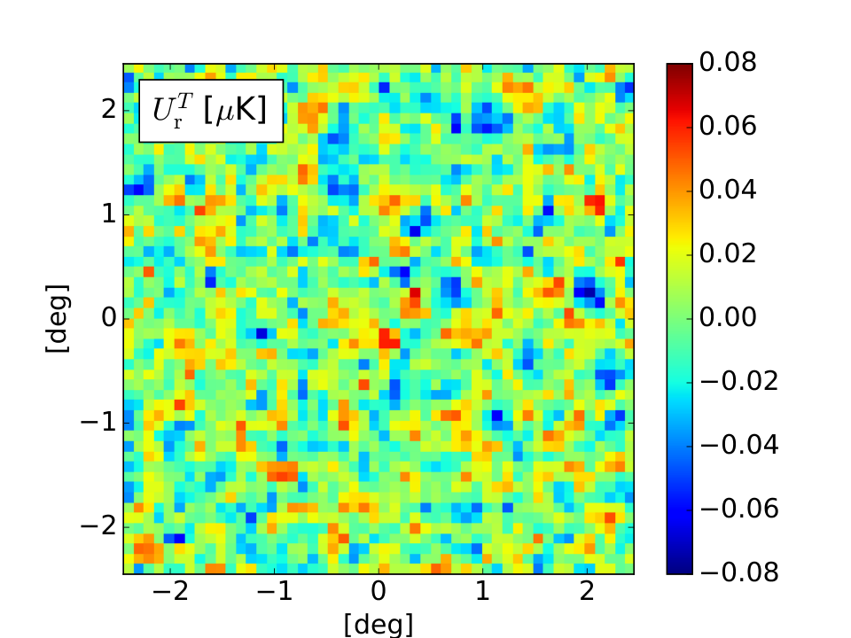
Firstly we note that as a basic check we have verified that Fig. 1 closely reproduces the stacked images shown in Planck Collaboration XVI (2016). We also show the and images stacked on -mode extrema in Fig. 2. The visually striking quadrupole pattern in appears to be an artefact of the pixelization scheme and is related to the so-called “sub-pixel” effects described in Planck Collaboration XV (2014) and Planck Collaboration XI (2016). This happens because the pixels of the stacked image are imperfectly separated near the centre of the map (the stacked image does not exhibit this imperfect mixing, because the pixel boundaries align perfectly with where the profile changes sign). The pixelization errors are more evident in the image than the because the individual and images are strongly peaked near the centre of the image, and thus when generating the stack imperfect subtraction leads to features in the centre of Fig. 2 (bottom). This effect has a non-diagonal influence on the power spectra and thus has a negligible effect on parameters (Planck Collaboration XV 2014) and this analysis. Alternatively, since constraints on come only from the radial part of the stacked images, the pixelization pattern seen in the centre of Fig. 2, which cancels out in the azimuthal average, will not bias our results (though it will contribute to the statistical uncertainty).
Fig. 3 shows the binned profiles for the four component-separation methods. The apparently non-zero signal seen in Fig. 3 is not visible in Figs. 1 and 2. This is mainly due to the fact that any signal in the stacked images must be shared out over the 2500 pixels and partially due to the fact that oscillates about zero for . The binning here is chosen to pick out ranges with the same sign in the predicted curve for (with the CDM prediction being identically zero); this choice is for visualization purposes only, since the statistical fit is performed on the original stacked images, i.e., Figs. 1 and 2.
Results are summarized in Table 1 and 2 for Commander, NILC, SEVEM, and SMICA. Table 1 contains the constraint on based on the high-pass-filtered and maps and their half-mission half differences (HMHD), which give a useful measure of the noise in the data. We present results based on stacking on temperature and -mode extrema, both separately and combined. We have estimated that the correlation of the temperature and -mode stacks are at the sub-percent level by looking at the amount of overlap in the positions of the peaks; thus we can safely neglect correlations in the combined fit. From Table 2 we can see that for most cases fits the data reasonably well; however, the reduction in from a non-zero is large enough, compared to the expectation of adding a single parameter, to yield a significant detection (with respect to statistical uncertainty only). In other words, while a horizontal line going through K might seem like an acceptable fit in Fig. 3, a non-zero is able to pick out the oscillatory features providing a significantly better fit. We report – detections for (with respect to statistical uncertainty only), however, this can be completely explained by a systematic rotation of our polarization-sensitive bolometers (PSBs) which we discuss in Sect. 6. Null-test estimates all give within 1 of 0∘, with the exception of Commander results stacked on temperature, which are slightly above (see the second and eighteenth rows of Table 1). We have also checked that there is very weak dependence on our results coming from the different choices for the thresholds used to define the peaks.
|
||||||||||||||||||||||||||||||||||||||||||||||||||||||||||||||||||||||||||||||||||||||||||||||||||||||||||||||||||
| aWe include the fit from each component-separation method’s half-mission half-difference (HMHD) and maps, as an indication of the expectation for noise. |
| bNILC and SMICA have smaller uncertainties compared with Commander and SEVEM, which follows from the naive expectation of the rms in the polarization maps (Planck Collaboration IX 2016, see table 1 of). |
|
|||||||||||||||||||||||||||||||||||||||||||||||||||||||||||||||||||||||||||||||||||||||||||||
| aThe number of degrees of freedom is 2500 coming from a patch with pixel size. |
A stacking analysis similar to ours has been attempted in Contaldi (2015) also using Planck data. Our results based on – data are consistent with those of Contaldi (2015), but with smaller statistical uncertainties; however, we disagree with Contaldi (2015) regarding the constraints coming from – data, which are claimed to be too noisy to be used. We show here that both – and – data can be successfully exploited to constrain the birefringence angle.
5.2 Harmonic-space results
Following the recommendation given by the Planck collaboration (Planck Collaboration IX 2016), we present results below based only on cross-correlations. Therefore, as described in Sect. 3, we present results for the -estimator using the full-mission data from Commander, NILC, SEVEM, and SMICA, and with half-mission data for SMICA. For the same reasons we present results with the -estimator using the half-mission data from SMICA only. Additionally we present a joint analysis with the half-mission data from SMICA. Of course the -estimators are built through the CMB angular power spectra. As an example, we display in Fig. 4 the and CMB angular power spectra obtained with the SMICA method using half-mission data. We also show the FFP8.1 simulations for the same component-separation method.
5.2.1 –
The estimates obtained are displayed in Fig. 5 as a function of the maximum multipole considered (). We note that all the estimates are stable among the component-separation methods and against the choice of . Moreover, the SMICA results provide a further test of stability with respect to computing the CMB angular power spectra from full-mission or half-mission data and simulations.
The estimates of the birefringence angle for are also reported in Table 3 (see first five rows for ).
|
|||||||||||||||||||||||||||||||||||||||||||||||||||||||||
| aThe bias refers to the average value of determined using the corresponding FFP8.1 simulations. |
| bNILC and SMICA have smaller uncertainties compared with Commander and SEVEM, which follows from the naive expectation of the rms in the polarization maps (Planck Collaboration IX 2016, see table 1 of). |
| cThe symbol denotes the cross-correlation of half-mission 1 with half-mission 2 data. |
| dThe corresponding probability to exceed is always below except for SEVEM which turns out to be . |
In Fig. 6 we show the dependence of on angular scale.99 9 This should not be confused with a spectrum of the birefringence anisotropies. As stated in Sect. 2 in this paper we are only concerned with a uniform rotation. This is built by considering Eq. (25) applied to . Comparing the different component-separation methods and the different ways of estimating the spectra, we find good stability of the estimates for each angular scale. The statistical uncertainties follow the behavior described in Gruppuso et al. (2016).
5.2.2 –
Considering Eq. (24) for the estimator , defined in Eq. (20), we have extracted the birefringence angle for the half-mission SMICA data. The estimate obtained for is given in Table 3 (see sixth row) and is compatible with constraints from the other component-separation methods, as is also clear from Fig. 5. Fig. 6 shows the spectrum of obtained in this case. Note that the statistical uncertainty coming from is much smaller than that obtained from . This is expected, since Eqs. (26) and (27) suggests that the – correlation is able to constrain better than the – correlation.
5.2.3 – and – combined
The CMB power spectra from the SMICA cross-correlations allow us to build a joint estimate minimizing the total , defined as . We have explicitly checked with FFP8.1 simulations that there is no significant cross-correlation between and 1010 10 The impact of taking such a cross-correlation into account is at most at the level of half of the statistical standard deviation. and this in turn means that it is possible to minimize the simple sum of . Not surprisingly, it turns out that such a combination is dominated by the – correlation information. The obtained constraint is reported again in Table 3 (see last row) and in Fig. 5. As before, in Fig. 6 we provide the spectrum of obtained from minimizing in intervals of . The overall consistency of each estimate is always very good.
6 Systematic effects
The main systematic effect that is completely degenerate with the signal from isotropic cosmological birefringence is uncertainty in the orientation of the PSBs used for mapmaking (Pagano et al. 2009). The nature of this error is characterized in the PCCS2 paper (Planck Collaboration XXVI 2016), as well as HFI (Planck Collaboration VII 2016; Planck Collaboration VIII 2016) and LFI (Leahy et al. 2010; Planck Collaboration III 2014; Planck Collaboration IV 2014) systematics papers, and also described in Planck Collaboration XLVI (2016). The present upper limit in any global rotation of the HFI detectors is estimated to be better than ; however, the relative upper limit between separate PSBs is (Rosset et al. 2010). After converting the above numbers into standard deviations (assuming they are approximately uniform distributions, and noting that the relative uncertainty can be averaged over the eight PSBs used by Planck) we conservatively quote the total (global and relative) 1 uncertainty as . This final error is not exactly Gaussian, although it is close (68 % and 95 % CLs are and , respectively). Given that we detect a rotation of around , we are, therefore, unable to disentangle the signal found in the data from the possible presence of this systematic effect. It remains to be seen whether or not this can be improved in a future Planck release.
It might be expected that Commander would perform best in polarization in terms of noise and handling of systematics (based on the angular scales probed here, see Planck Collaboration IX 2016, for details). However, given that Commander uses a slightly different set of data than the other component-separation methods and given that they all use different algorithms, we cannot make any definitive claims as to which gives the most accurate constraint. We are also unable to account for the apparent discrepancy at the roughly 2 level (given the large number of comparisons performed here, this could simply be a statistical fluke) that the Commander noise estimate yields for when stacking on temperature (see Table 1). That being said, it is reassuring that all component-separation methods agree at the level in their constraints on .
In the following subsections we mention some other possible systematic effects that might be present, but that we believe contribute negligibly to the polarization rotation signal.
6.1 Noise properties of polarization
The recommendation from the Planck collaboration is that any analysis performed on polarization data should not be very sensitive to mis-characterization of the noise. To this end cross-spectra, cross-correlation, and stacking analyses are examples of such approaches. Our harmonic space and map space temperature tests fulfil this criterion explicitly. It is less obvious that stacking on -mode extrema should only weakly depend on the noise properties; however, we find this to be the case. This is because the statistics of the -mode map are encoded in the bias parameters (), which depend on the total power in the map (see Appendix A for details). Therefore the bias parameters will be accurate to the level that the statistics of the polarization data can be determined by its two-point function. Nevertheless we will now describe to what extent a miscalculation of the bias parameters will affect our results.
We use the MASTER method (Hivon et al. 2002, to correct for masking,) to estimate the total power spectrum of the -mode map in order to calculate the bias parameters (). The noise term in Eq. (11) is then given by subtracting the theoretical power spectrum () from the total power spectrum. The main effect of noise, however, comes from the determination of the bias terms only, since most of the discriminatory power on comes from the stacks (Eqs. 12 and 16 do not explicitly depend on the noise term).
The largest difference in our noise estimation when comparing between different component-separation methods comes from SEVEM and SMICA. For these maps differs by approximately %, and by %. Using the SEVEM bias parameter values on the SMICA data (for example) leads to a roughly shift in the posterior of (from -modes). Such a discrepancy estimate is overly conservative however, because each component-separation technique will generally produce maps with different noise levels. If instead we scale our noise estimate by as much as 10 % (for any of the individual component-separation methods) we find that shifts by less than 0.25. We therefore conclude that for our analysis, mis-characterization of the noise in polarization has little to no effect.
6.2 Beam effects
Because of the differential nature of polarization measurements, any beam mismatch or uncertainties can induce temperature-to-polarization leakage (Hu et al. 2003; Leahy et al. 2010). Here we are interested in beam uncertainties that can potentially lead to – and – correlations that might mimic a non-zero signal. Due to circular symmetry, effects from differential beam sizes or differential relative gains will not tend to produce – or – correlations, whereas effects from differential pointing and differential ellipticity will. Differences in the noise level will also in general cause temperature-to-polarization leakage.
We check for these effects following the approach described in Planck Collaboration XI (2016) and Planck Collaboration XIII (2016). Note that temperature-to-polarization leakage estimates due to bandpass mismatches between detectors have been removed from the component-separated maps (see Planck Collaboration IV 2016; Planck Collaboration VI 2016; Planck Collaboration VIII 2016; Planck Collaboration IX 2016, for details); we perform a crude scan of the parameter space in the following temperature-to-polarization leakage model (Planck Collaboration XLVI 2016, see also appendix A.6 of):
| (28) | ||||
| (29) | ||||
| (30) | ||||
| (31) |
The and terms are expected to be dominated by and modes (assuming the mismatch comes from differential ellipticity) and can be written as
| (32) | ||||
| (33) |
Varying , and in the range given by , and (Planck Collaboration XI 2016), we find that is stable to (this is the case for both temperature and -mode stacks).
We must stress, however, that the above temperature-to-polarization leakage model is not completely satisfactory (see section 3.4.3 and appendix C.3.5 in Planck Collaboration XI 2016, for full details). Nevertheless it is adequate for our purposes, since we only wish to demonstrate that our results remain stable to most forms of beam mismatch.
7 Conclusions
We have estimated the rotation, , of the plane of polarization of CMB photons by using Planck 2015 data. Employing harmonic-space cross-correlations and a map-space stacking approach we find values of and , respectively, for the angle (using SMICA data). Both methods yield the same statistical uncertainty, i.e., (68 % CL), and are subject to the same systematic error of (68 % CL) due to the uncertainty in the global and relative orientations of the PSBs. Our results are compatible with no rotation, i.e., no parity violation, within the total error budget. We have demonstrated that our findings are robust against two independent analysis approaches, different component-separation methods, harmonic scales, choices in peak thresholds, and temperature-to-polarization leakage, at better than the statistical level. We have also carefully chosen our analyses to be insensitive to detailed knowledge of the noise properties of the polarization data. Note that the statistical and systematic error bars represent our best knowledge of the Planck data at the time of publication.1111 11 We do not recommend the use of any , and information (either in form of spectra, stacking or any other estimator that depends on the cross-correlation between and modes or and modes) without including in the analysis the uncertainty coming from the instrumental polarization angle (and other systematic effects that might dominate the error budget). Several additional effects have the potential to enlarge the error estimates. Among the possible source of extra systematics are residuals from the processing, which are only partially captured by the FFP8.1 simulations since these simulations do not yet include all the details of the instruments. In Planck Collaboration XI (2016) we analysed a few end-to-end simulations from HFI, which include more systematic effects than those contained in FFP8.1, and found no evidence for significant influence on the results of the TT likelihood. Planck Collaboration XLVI (2016) shows that the FFP8 simulations fail to capture most of the very low ell () polarization systematics. Our measurement here, based on multipoles larger than should be immune to these sorts of issues, but there are not enough end-to-end simulations available at this time to definitively prove this. Similarly, we relied on the efficiency of component-separated maps to treat the Galactic residuals. This assumes that the FFP8 Galactic model correctly describes and induced correlation. Comparing the estimates obtained from different component-separation methods, we expect that the latter uncertainty is at most of the order the of statistical error.
In Fig. 8 we show a comparison of our estimate with the birefringence angle estimates provided by analysis on other CMB data in which, where possible, the total error budget is decomposed in these two parts, i.e. statistical (left point of a pair) and systematic (right).
The total error budget of our estimate is dominated by the systematic uncertainty, which is a factor of 6 larger than the statistical one. It is clear, therefore, that future CMB polarization experiments (or a future Planck release) will require a much better understating of their polarimeter orientations, since this is appearing as the current limiting factor of this investigation. With a coordination of careful ground-based measurements and improved in-flight calibration on polarized sources (see Kaufman et al. 2014, for an example of a possible effort) we may be able to further probe possible parity violations in the Universe.
Acknowledgements.
The Planck Collaboration acknowledges the support of: ESA; CNES, and CNRS/INSU-IN2P3-INP (France); ASI, CNR, and INAF (Italy); NASA and DoE (USA); STFC and UKSA (UK); CSIC, MINECO, JA, and RES (Spain); Tekes, AoF, and CSC (Finland); DLR and MPG (Germany); CSA (Canada); DTU Space (Denmark); SER/SSO (Switzerland); RCN (Norway); SFI (Ireland); FCT/MCTES (Portugal); ERC and PRACE (EU). A description of the Planck Collaboration and a list of its members, indicating which technical or scientific activities they have been involved in, can be found at http://www.cosmos.esa.int/web/planck/planck-collaboration. Some of the results of this paper have been derived using the HEALPix package (Górski et al. 2005).References
- Ade et al. (2014a) Ade, P. A. R. et al., A Measurement of the Cosmic Microwave Background B-Mode Polarization Power Spectrum at Sub-Degree Scales with POLARBEAR. 2014a, ApJ, 794, 171, 1403.2369
- Ade et al. (2014b) Ade, P. A. R. et al., BICEP2 II: Experiment and Three-Year Data Set. 2014b, ApJ, 792, 62, 1403.4302
- Ade et al. (2015) Ade, P. A. R. et al., POLARBEAR Constraints on Cosmic Birefringence and Primordial Magnetic Fields. 2015, Phys. Rev., D92, 123509, 1509.02461
- Bielewicz et al. (2012) Bielewicz, P., Banday, A. J., & Górski, K. M., Constraining the topology of the Universe using the polarized cosmic microwave background maps. 2012, MNRAS, 421, 1064, 1111.6046
- Bond & Efstathiou (1987) Bond, J. R. & Efstathiou, G., The statistics of cosmic background radiation fluctuations. 1987, MNRAS, 226, 655
- Brown et al. (2009) Brown, M. L., Ade, P., Bock, J., et al., Improved Measurements of the Temperature and Polarization of the Cosmic Microwave Background from QUaD. 2009, ApJ, 705, 978, 0906.1003
- Carroll (1998) Carroll, S. M., Quintessence and the Rest of the World: Suppressing Long-Range Interactions. 1998, Phys. Rev. Lett., 81, 3067, astro-ph/9806099
- Carroll et al. (1990) Carroll, S. M., Field, G. B., & Jackiw, R., Limits on a Lorentz- and parity-violating modification of electrodynamics. 1990, Phys. Rev. D, 41, 1231
- Cimatti et al. (1994) Cimatti, A., de Serego Alighieri, S., Field, G. B., & Fosbury, R. A. E., Stellar and scattered light in a radio galaxy at = 2.63. 1994, ApJ, 422, 562
- Cimatti et al. (1993) Cimatti, A., di Serego-Alighieri, S., Fosbury, R. A. E., Salvati, M., & Taylor, D., Optical Polarization in Distant Radio Galaxies. 1993, MNRAS, 264, 421
- Contaldi (2015) Contaldi, C. R., Imaging parity-violation in the CMB. 2015, ArXiv e-prints, 1510.02629
- Desjacques (2008) Desjacques, V., Baryon acoustic signature in the clustering of density maxima. 2008, Phys. Rev. D, 78, 103503, 0806.0007
- di Serego Alighieri et al. (2010) di Serego Alighieri, S., Finelli, F., & Galaverni, M., Limits on Cosmological Birefringence from the Ultraviolet Polarization of Distant Radio Galaxies. 2010, ApJ, 715, 33, 1003.4823
- di Serego Alighieri et al. (2014) di Serego Alighieri, S., Ni, W.-T., & Pan, W.-P., New Constraints on Cosmic Polarization Rotation From B-mode Polarization in the Cosmic Microwave Background. 2014, ApJ, 792, 35, 1404.1701
- Feng et al. (2005) Feng, B., Li, H., Li, M., & Zhang, X., Gravitational leptogenesis and its signatures in CMB. 2005, Physics Letters B, 620, 27, hep-ph/0406269
- Feng et al. (2006) Feng, B., Li, M., Xia, J.-Q., Chen, X., & Zhang, X., Searching for CPT Violation with Cosmic Microwave Background Data from WMAP and BOOMERANG. 2006, Phys. Rev. Lett., 96, 221302, astro-ph/0601095
- Finelli & Galaverni (2009) Finelli, F. & Galaverni, M., Rotation of Linear Polarization Plane and Circular Polarization from Cosmological Pseudo-Scalar Fields. 2009, Phys. Rev., D79, 063002, 0802.4210
- Gluscevic et al. (2012) Gluscevic, V., Hanson, D., Kamionkowski, M., & Hirata, C. M., First CMB Constraints on Direction-Dependent Cosmological Birefringence from WMAP-7. 2012, Phys. Rev., D86, 103529, 1206.5546
- Górski et al. (2005) Górski, K. M., Hivon, E., Banday, A. J., et al., HEALPix: A Framework for High-Resolution Discretization and Fast Analysis of Data Distributed on the Sphere. 2005, ApJ, 622, 759, astro-ph/0409513
- Gruppuso et al. (2015) Gruppuso, A., Gerbino, M., Natoli, P., et al., Constraints on cosmological birefringence from Planck and Bicep2/Keck data. 2015, ArXiv e-prints, 1509.04157
- Gruppuso et al. (2016) Gruppuso, A., Maggio, G., Molinari, D., & Natoli, P., A note on the birefringence angle estimation in CMB data analysis. 2016, JCAP, 1605, 020
- Gruppuso et al. (2012) Gruppuso, A., Natoli, P., Mandolesi, N., et al., WMAP 7 year constraints on CPT violation from large angle CMB anisotropies. 2012, JCAP, 1202, 023, 1107.5548
- Gubitosi et al. (2014) Gubitosi, G., Martinelli, M., & Pagano, L., Including birefringence into time evolution of CMB: current and future constraints. 2014, J. Cosmology Astropart. Phys., 12, 20, 1410.1799
- Hinshaw et al. (2013) Hinshaw, G. et al., Nine-Year Wilkinson Microwave Anisotropy Probe (WMAP) Observations: Cosmological Parameter Results. 2013, Astrophys. J. Suppl., 208, 19, 1212.5226
- Hivon et al. (2002) Hivon, E., Górski, K. M., Netterfield, C. B., et al., MASTER of the Cosmic Microwave Background Anisotropy Power Spectrum: A Fast Method for Statistical Analysis of Large and Complex Cosmic Microwave Background Data Sets. 2002, ApJ, 567, 2, astro-ph/0105302
- Hu et al. (2003) Hu, W., Hedman, M. M., & Zaldarriaga, M., Benchmark parameters for CMB polarization experiments. 2003, Phys. Rev. D, 67, 043004, astro-ph/0210096
- Kamionkowski (2010) Kamionkowski, M., Nonuniform cosmological birefringence and active galactic nuclei. 2010, Phys. Rev. D, 82, 047302, 1004.3544
- Kamionkowski et al. (1997) Kamionkowski, M., Kosowsky, A., & Stebbins, A., Statistics of cosmic microwave background polarization. 1997, Phys. Rev. D, 55, 7368, astro-ph/9611125
- Kaufman et al. (2016) Kaufman, J. P., Keating, B. G., & Johnson, B. R., Precision Tests of Parity Violation over Cosmological Distances. 2016, Mon. Not. Roy. Astron. Soc., 455, 1981, 1409.8242
- Kaufman et al. (2014) Kaufman, J. P., Miller, N. J., Shimon, M., et al., Self-calibration of BICEP1 three-year data and constraints on astrophysical polarization rotation. 2014, Phys. Rev. D, 89, 062006, 1312.7877
- Keating et al. (2012) Keating, B., Shimon, M., & Yadav, A., Self-Calibration of CMB Polarization Experiments. 2012, Astrophys. J., 762, L23, 1211.5734
- Kim (2011) Kim, J., How to make a clean separation between CMB E and B modes with proper foreground masking. 2011, A&A, 531, A32, 1010.2636
- Kogut et al. (2003) Kogut, A., Spergel, D. N., Barnes, C., et al., First-Year Wilkinson Microwave Anisotropy Probe (WMAP) Observations: Temperature-Polarization Correlation. 2003, ApJS, 148, 161, astro-ph/0302213
- Komatsu et al. (2011) Komatsu, E., Smith, K. M., Dunkley, J., et al., Seven-year Wilkinson Microwave Anisotropy Probe (WMAP) Observations: Cosmological Interpretation. 2011, ApJS, 192, 18, 1001.4538
- Leahy (1997) Leahy, J. P., Comment on the Measurement of Cosmological Birefringence. 1997, ArXiv Astrophysics e-prints, astro-ph/9704285
- Leahy et al. (2010) Leahy, J. P., Bersanelli, M., D’Arcangelo, O., et al., Planck pre-launch status: Expected LFI polarisation capability. 2010, A&A, 520, A8
- Li et al. (2009) Li, M., Cai, Y.-F., Wang, X., & Zhang, X., CPT violating electrodynamics and Chern-Simons modified gravity. 2009, Physics Letters B, 680, 118, 0907.5159
- Li & Zhang (2008) Li, M. & Zhang, X., Cosmological CPT violating effect on CMB polarization. 2008, Phys. Rev., D78, 103516, 0810.0403
- Liu et al. (2006) Liu, G.-C., Lee, S., & Ng, K.-W., Effect on cosmic microwave background polarization of coupling of quintessence to pseudoscalar formed from the electromagnetic field and its dual. 2006, Phys. Rev. Lett., 97, 161303, astro-ph/0606248
- Lue et al. (1999) Lue, A., Wang, L., & Kamionkowski, M., Cosmological Signature of New Parity-Violating Interactions. 1999, Phys. Rev. Lett., 83, 1506, astro-ph/9812088
- Mei et al. (2015) Mei, H.-H., Ni, W.-T., Pan, W.-P., Xu, L., & di Serego Alighieri, S., New Constraints on Cosmic Polarization Rotation from the ACTPol Cosmic Microwave Background B-mode Polarization Observation and the BICEP2 Constraint Update. 2015, ApJ, 805, 107, 1412.8569
- Molinari et al. (2016) Molinari, D., Gruppuso, A., & Natoli, P., Constraints on parity violation from ACTpol and forecasts for forthcoming CMB experiments. 2016, 1605.01667
- Naess et al. (2014) Naess, S., Hasselfield, M., McMahon, J., et al., The Atacama Cosmology Telescope: CMB polarization at . 2014, J. Cosmology Astropart. Phys., 10, 7, 1405.5524
- Pagano et al. (2009) Pagano, L., de Bernardis, P., de Troia, G., et al., CMB polarization systematics, cosmological birefringence, and the gravitational waves background. 2009, Phys. Rev. D, 80, 043522, 0905.1651
- Planck Collaboration III (2014) Planck Collaboration III, Planck 2013 results. III. LFI systematic uncertainties. 2014, A&A, 571, A3, 1303.5064
- Planck Collaboration IV (2014) Planck Collaboration IV, Planck 2013 results. IV. LFI Beams and window functions. 2014, A&A, 571, A4, 1303.5065
- Planck Collaboration XV (2014) Planck Collaboration XV, Planck 2013 results. XV. CMB power spectra and likelihood. 2014, A&A, 571, A15, 1303.5075
- Planck Collaboration I (2016) Planck Collaboration I, Planck 2015 results. I. Overview of products and results. 2016, A&A, submitted, 1502.01582
- Planck Collaboration IV (2016) Planck Collaboration IV, Planck 2015 results. IV. LFI beams and window functions. 2016, A&A, in press, 1502.01584
- Planck Collaboration VI (2016) Planck Collaboration VI, Planck 2015 results. VI. LFI maps. 2016, A&A, submitted, 1502.01585
- Planck Collaboration VII (2016) Planck Collaboration VII, Planck 2015 results. VII. High Frequency Instrument data processing: Time-ordered information and beam processing. 2016, A&A, in press, 1502.01586
- Planck Collaboration VIII (2016) Planck Collaboration VIII, Planck 2015 results. VIII. High Frequency Instrument data processing: Calibration and maps. 2016, A&A, in press, 1502.01587
- Planck Collaboration IX (2016) Planck Collaboration IX, Planck 2015 results. IX. Diffuse component separation: CMB maps. 2016, A&A, submitted, 1502.05956
- Planck Collaboration X (2016) Planck Collaboration X, Planck 2015 results. X. Diffuse component separation: Foreground maps. 2016, A&A, submitted, 1502.01588
- Planck Collaboration XI (2016) Planck Collaboration XI, Planck 2015 results. XI. CMB power spectra, likelihoods, and robustness of parameters. 2016, A&A, submitted, 1507.02704
- Planck Collaboration XII (2016) Planck Collaboration XII, Planck 2015 results. XII. Full Focal Plane simulations. 2016, A&A, submitted, 1509.06348
- Planck Collaboration XIII (2016) Planck Collaboration XIII, Planck 2015 results. XIII. Cosmological parameters. 2016, A&A, submitted, 1502.01589
- Planck Collaboration XVI (2016) Planck Collaboration XVI, Planck 2015 results. XVI. Isotropy and statistics of the CMB. 2016, A&A, in press, 1506.07135
- Planck Collaboration XXVI (2016) Planck Collaboration XXVI, Planck 2015 results. XXVI. The Second Planck Catalogue of Compact Sources. 2016, A&A, submitted, 1507.02058
- Planck Collaboration XLVI (2016) Planck Collaboration XLVI, Planck intermediate results. XLVI. Reduction of large-scale systematic effects in HFI polarization maps and estimation of the reionization optical depth. 2016, A&A, submitted, 1605.02985
- Polenta et al. (2005) Polenta, G., Marinucci, D., Balbi, A., et al., Unbiased estimation of an angular power spectrum. 2005, J. Cosmology Astropart. Phys., 11, 1, astro-ph/0402428
- Rosset et al. (2010) Rosset, C., Tristram, M., Ponthieu, N., et al., Planck pre-launch status: High Frequency Instrument polarization calibration. 2010, A&A, 520, A13, 1004.2595
- Wardle et al. (1997) Wardle, J. F. C., Perley, R. A., & Cohen, M. H., Observational Evidence against Birefringence over Cosmological Distances. 1997, Phys. Rev. Lett., 79, 1801, astro-ph/9705142
- Wu et al. (2009) Wu, E. Y. S., Ade, P., Bock, J., et al., Parity Violation Constraints Using Cosmic Microwave Background Polarization Spectra from 2006 and 2007 Observations by the QUaD Polarimeter. 2009, Phys. Rev. Lett., 102, 161302, 0811.0618
- Zaldarriaga & Seljak (1997) Zaldarriaga, M. & Seljak, U., All-sky analysis of polarization in the microwave background. 1997, Phys. Rev. D, 55, 1830, astro-ph/9609170
- Zhao et al. (2015) Zhao, G.-B., Wang, Y., Xia, J.-Q., Li, M., & Zhang, X., An efficient probe of the cosmological CPT violation. 2015, JCAP, 1507, 032, 1504.04507
Appendix A Stacking on -mode peaks
Here we will discuss the new procedure of stacking on -mode extrema. We remind readers that the full implementation and derivation of all relevant parameters are discussed in great detail in appendix B of Komatsu et al. (2011), and a similar derivation is given in Contaldi (2015) for stacking on and extrema. Here we simply explain the few details required to extend the formalism for stacking on -modes.
Selecting the peaks of an underlying Gaussian field (like or ) leads to a biased selection of that field. Such a bias is scale-dependent and has the form
| (34) |
The scale-dependent term () arises because peaks are defined by a vanishing first derivative and the sign of the second derivative (Desjacques 2008).
The bias parameters depend entirely on rms values of derivatives of the Gaussian field, , and (Bond & Efstathiou 1987, they also depend on special functions involved in translating a 3-dimensional Gaussian random field to the 2-dimensional case, as discussed in). These are defined as
| (35) | ||||
| (36) |
This is the only expression that contains the noise term , which is why understanding the noise properties of the -mode map is potentially considered to be a relevant systematic effect (see Sect. 6.1).
When we stack or on the location of -mode peaks we are explicitly computing the cross-correlation or . Recalling that both and can be written in terms of and -mode contributions (Zaldarriaga & Seljak 1997; Kamionkowski et al. 1997) and rewriting Eq. (34) in the flat-sky approximation we arrive at1212 12 For brevity we henceforth drop the noise term in the expression for .
| (37) | |||
| (38) |
Here we have used the coordinate convention of Komatsu et al. (2011), thus , and . We can perform the internal integration over using properties of Bessel functions to finally arrive at Eqs. (11)–(12), i.e.,
| (39) | ||||
| (40) |