Local Region Sparse Learning for Image-on-Scalar Regression

Regression models with image responses and scalar predictors are routinely encountered in many applications [2, 7]. Consider an image-on-scalar regression model with varying coefficients: $Y(s)=X^{T}\beta(s)+\eta(s)+\epsilon(s)$, where $X\in\mathbb{R}^{p}$ is the covariate, $Y(s)\in\mathbb{R}$ is the image response at pixel $s\in{\cal S}$ (a 2D or 3D domain), and $\beta(s)=(\beta_{1}(s),\ldots,\beta_{p}(s))^{T}\in\mathbb{R}^{p}$ is the coefficient image vector. Here $\eta(\cdot)$ is a zero-mean spatial field which characterizes the spatial correlation, and $\epsilon(\cdot)$ is the white noise with mean zero and variance $\sigma^{2}$. In this paper, we focus on $Y\in\mathbb{R}^{N\times N}$ a 2D image. Extension to 3D images is straightforward. The objective is to identify ROI in the response image which are associated with the corresponding covariate by estimating the coefficient images $\beta_{1},\ldots,\beta_{p}$. The available data are image and covariate pairs for $n$ subjects, $(X_{i},Y_{i}(\cdot))$, $i=1,\ldots,n$. We obtain the estimator by minimizing

where $\mbox{pen}(\cdot)$ is a penalty function which favors estimators according to certain criteria. Our purpose is to recover nonzero active regions of $\beta_{1},\ldots,\beta_{p}$. The main challenges are that we need to impose sparsity of pixel values and extract active regions simultaneously.

TV and SCAD. The TV analysis plays a fundamental role in various image analyses since the path-breaking works [13, 12]. We focus on the anisotropic version of TV. For $\beta\in\mathbb{R}^{N\times N}$, define the discrete gradient $\nabla:\mathbb{R}^{N\times N}\rightarrow\mathbb{R}^{N\times N\times 2}$ is defined by

The TV norm $\|\beta\|_{TV}$ is just $\|\beta\|_{TV}=\sum_{j,k}\|(\nabla\beta)_{jk}\|_{1}$. The isotropic induced TV norm is $\sum_{j,k}\|(\nabla\beta)_{jk}\|_{2}$, which is equivalent to the anisotropic induced TV norms up to a factor of $\sqrt{2}$.

The SCAD penalty $\rho_{\lambda}(\cdot)$ is more conveniently defined its derivative

and $\rho_{\lambda}(0)=0$. We use $a=3.7$ by convention. Consider a penalized least squares problem: minimize ${\varrho\over 2}(z-\theta)^{2}+\rho_{\lambda}(\theta)$. The solution is unique, explicit, and $\hat{\theta}=S_{\varrho,\lambda}(z)$, where $S_{\varrho,\lambda}$ is the thresholding function. Figure 1 displays the thresholding function for SCAD and the soft thresholding function for Lasso with $\varrho=1$ and $\lambda=2$. The SCAD penalty shrinks small coefficients to zero while keeping the large coefficients without shrinkage.

GraphNet and TV-$\ell_{1}$. GraphNet and TV-$\ell_{1}$ have been successful applied to medical images. GraphNet is the weighted average of an $\ell_{1}$ penalty on all coordinates and a squared $\ell_{2}$ penalty on the discrete gradient, while TV-$\ell_{1}$ is the weighted average of an $\ell_{1}$ penalty and a TV penalty:

For both penalties, $\lambda>0$ is the smoothing parameter which controls the strength of regularization and $\gamma\in[0,1]$ is another smoothing parameter controlling the trade-off between pixel sparsity and spatial regularity.

For each coordinate $\beta_{jk}$, the discrete gradient $(\nabla\beta)_{jk}\in\mathbb{R}^{2}$ involves three coordinate values $\beta_{jk},\beta_{j+1,k},\beta_{j,k+1}$. Let $\widetilde{\beta}_{jk}=(\beta_{jk},\beta_{j+1,k},\beta_{j,k+1})^{T}$. The SCAD2TV penalty is defined by

where $\lambda>0$ and $\gamma\in[0,1]$ are two tuning parameters, and $\rho_{\lambda}$ is the SCAD function. The first term in the penalty allows adaptive estimation of the coefficient image and the second one enforces sparsity on coordinate values. One may also consider the functional version of (2). After some rescaling, (2) is equivalent to

The SCAD2TV solves the bias problem inherent in the TV and Lasso models. Note that this penalty function, unlike the $L_{1}$ penalty used in Lasso, is not convex, so that (1) is a non-convex objective function. We solve this problem based on the ADMM and convert it into two sub-problems with closed-form solutions. In general, ADMM has successful applications to convex problems. The behavior of ADMM applied to nonconvex problems has been a mystery. Recently, the global convergence of ADMM in non-convex optimization is discussed in [17], which shows that several ADMM algorithms including SCAD are guaranteed to converge.

Our proposed algorithm is based on ADMM [1]. We may write (1) as the matrix form by an abuse of notation:

where $Y_{i}\in\mathbb{R}^{N^{2}}$ is the veritorized response image for subject $i$, $X_{i}\in\mathbb{R}^{N^{2}\times pN^{2}}$ is the fixed extended design matrix related to the covariate for subject $i$, and $\beta\in\mathbb{R}^{pN^{2}}$ is the concatenated vectorized unknown coefficient image. Furthermore, one of the advantages of SCAD2TV in (2) is that we can write $\sum_{j=1}^{p}\mbox{pen}_{S2TV}(\beta_{j})$ as $\|\rho_{\lambda}(D\beta)\|_{1}$ for a fixed $p(5(N-1)^{2}+6(N-1))$ by $pN^{2}$ matrix $D$ depending only on $\gamma$, which greatly facilitates the efficiency of our algorithm. This fact can be easily seen since the elements involved in the $(j,k)^{th}$ term in (2) are

for a fixed matrix $D_{jk}$. So $D$ is the concatenated version of $D_{jk}$.

Problem (4) is equivalent to

We form the augmented Lagrangian as

The ADMM consists of the iterations

It should be emphasized that both (5) and (6) have the explicit solutions. Specifically, (5) is a ridge regression problem and (6) is a penalized least squares problem with the identity design matrix. The closed-form solutions for (5) and 6 are, respectively,

The details of the algorithm is summarized in Algorithm 1.

The output is either $\beta$ or $\alpha$. Note that $\alpha$ is a sparse solution and $\beta$ may not be sparse. In practice, we extract the coefficient image estimator from the output $\alpha$ to obtain the sparse estimator.

To address the big data issue, a divide and conquer (D&C) algorithm is a solution by recursively breaking down a problem into two or more sub-problems of the same or related type, until these become simple enough to be solved directly. The solutions to the sub-problems are then combined to give a solution to the original problem. In the above discussion, we assume that, for each subject $i$, all image coordinate values $Y_{i}\in\mathbb{R}^{N^{2}}$ are used together to infer the coefficient images $\beta$. However, in many applications $N$ may be large and such a “batch” procedure is undesirable. In order to solve this issue, we develop a D&C algorithm for large image size.

Image data have their intrinsic structure and we need proceed the divide step with extra caution. For example, we may just partition each image as non-overlap sub-images $Y_{i}=Y_{i1}\cup Y_{i2}\cup\cdots\cup Y_{iJ}$, with the data processed sequentially. Due to the TV term in SCAD2TV, we lose the boundary information for all sub-images and this will give poor estimates of the boundary for all sub-images. We propose to partition $Y_{i}$ with overlapped sub-images $Y_{i}=\tilde{Y}_{i1}\cup\tilde{Y}_{i2}\cup\cdots\cup\tilde{Y}_{iJ}$. For instance, Figure 2 displays a $24\times 24$ image, and it is straightforward to partition them into nine non-overlapped $8\times 8$ sub-images. For our purpose, we extend each sub-image in four directions. Specifically, on the left up corner, we include both the light blue part and the light yellow part, which makes our first sub-image a $9\times 9$ image. In the center, we take the inside $8\times 8$ orange part together with the brown part, which makes it a $10\times 10$ image. After this partition, we obtain nine overlapped sub-images. We perform Algorithm 1 on each sub-image and update the coefficient images. For each update we only keep the estimate for the original $8\times 8$ sub-image.

The above D&C algorithm can be executed sequentially in a single machine. This algorithm is naturally adapted for execution in multi-processor machines, especially shared-memory systems where the communication of data between processors does not need to be planned in advance, because distinct sub-problems can be executed on different processors.

We design a synthetic data example to compare the performance among three approaches: SCAD2TV, GraphNet, and TV-$\ell_{1}$ in terms of both prediction and selection errors.

Data Generation. In our setting, $\beta=(\beta_{0},\beta_{1},\beta_{2})$ where each $\beta_{j}$ is a $64\times 64$ image (See the left panel of Figure 3). The covariate is $X=(1,X_{1},X_{2})^{T}$ and each $X_{j}$ is generated from a uniform distribution between $0$ and $2$. The spatial field $\eta(\cdot)$ is generated from a zero mean Gaussian random field. The error process $\epsilon(\cdot)$ is the white noise with mean zero and variance $\sigma^{2}$. Two noise levels are adopted at $\sigma=1,0.1$. The sample size is $n=100$.

Applying SCAD2TV. In order to examine the performances of three methods, SCAD2TV, GraphNet, and TV-$\ell_{1}$, we have generated $100$ datasets for each setting. For each dataset, we obtain the coefficient image estimates $\hat{\beta}$ from these three methods. The selection rate is define as

and the mean squared error is defined as

where $|S|=4096$ is the total number of pixels and the $\hat{Y}_{i}$ are the predicted images.

Practical Consideration. Smoothing parameters $\lambda,\gamma$ can be selected by using the K-fold cross-validation (CV). However, its computational time can be long even under current computing facilities. In our experiment, we have tested a few different values for the tuning parameters such as $\lambda=1,2,\ldots,10$ and $\gamma=0.1,0.2,\ldots,0.9$. We find $\gamma=0.5$ is a good balance for the estimation. The value of $\lambda$ is related to our expectation of ROI. If the ROI has a sharp boundary and the values do not change much inside ROI, we can use a large $\lambda$. Otherwise, a smaller $\lambda$ would be preferred. We choose $\lambda=5$, $\gamma=0.5$ and $\rho=1$.

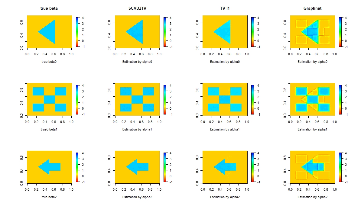
Results. For each setting, the experiments using SCAD2TV, GraphNet, TV-$\ell_{1}$ are repeated $100$ times. Figure 3 displays the estimates of coefficient images from one realization. We note that SCAD2TV provides the solution almost exact the same as the truth. TV-$\ell_{1}$ can keep the sharp boundary but provide biased estimates inside the active zone. GraphNet displays blurred estimates for both active zone and zero sub-regions. The average of the selection rates and the MSEs are reported in Table 1. It is noted that, in terms of the selection rate, SCAD2TV performs better consistently than the other two methods. On the other hand, in terms of the prediction error, SCAD2TV and TV-$\ell_{1}$ are similar to each other, and GraphNet gives the highest MSE.

Dataset. To illustrate the usefulness of our proposed model, consider anatomical MRI data collected at the baseline by the Alzheimer’s Disease Neuroimaging Initiative (ADNI) study, which is a large scale multi-site study collecting clinical, imaging, and laboratory data at multiple time points from healthy controls, individuals with amnestic mild cognitive impairment, and subjects with Alzheimer’s disease. Given the MRI scans, hippocampal substructures were segmented with FSL FIRST [11] and hippocampal surfaces were automatically reconstructed with the marching cube method [8]. We adopted a surface fluid registration based hippocampal subregional analysis package [14], which uses isothermal coodinates and uid registration to generate one-to-one hippocampal surface registration for surface statistics computation.

In the dataset, we have total $403$ observations. For each subject, it includes a $150\times 100$ 2D representation of left hippocampus and $4$ covariates: gender (female=0 and male=1), age (55-92), disease status (control=0 and AD=1), and behavior score (1-36). The goal is to identify local regions of the response image associated with each covariate.

Applying SCAD2TV. We have applied our D&C learning algorithm to this dataset. We divide each response image into $150$ overlapped sub-images. We execute the algorithm sequentially in a single machine. The algorithm spends about 10 secs for each partition, and takes 25 minutes to get the final estimation of $\beta$’s. The estimated coefficient images are presented in the top panel of Figure 4.

Results. Our purpose is to identify the local regions where the response hippocampus image is associated with each individual covariate. Among all of the covariates, we are particularly interested in the association between the response hippocampus image and the disease status (Control vs AD). From the top panel of Figure 4, it is interesting to notice that gender has no effect on the response image, and for other three covariates SCAD2TV has been successfully identify the local active regions.

We take a close investigation on the coefficient image corresponding to the disease status. The left panel of Figure 5 displays the estimate of $\beta_{3}$. The sub-regions in red indicate the active zone and the region in orange is the zero sub-region. In general, the AD patients have lower pixel values in the response hippocampus image. The right two panels are the mean response images for both health control and AD. The mean difference is consistent with our estimation of $\beta_{3}$.

We extract the pixels within the ROI for health controls and AD, and apply hypothesis testing to test if their difference is significant. By applying hypothesis testing on each pixel in the ROI, all of them are different between health controls and AD at the significance level $5\%$, and $99.85\%$ of the pixels in the ROI are different at the significance level $1\%$. The result justifies our ROI selection is indeed the region to differentiate between health controls and AD.

Comparison with TV-$\ell_{1}$ and GraphNet. We obtain the estimates of the coefficient images for TV-$\ell_{1}$ and GraphNet, which are presented in the middle and bottom panels of Figure 4. These three methods overall detects similar regions. Both TV-$\ell_{1}$ and GraphNet display more blocky active regions, whereas SCAD2TV keep the active zone with sharp boundaries. We also divide our dataset into 5 parts to compare the prediction performance where each dataset contains around 80 observations. Every time we use 4 of them as the training data, and make prediction on the remaining testing data. The averages of the MSEs are computed for each methods, which are reported in Table 2. The MSEs are similar to each other and SCAD2TV displays a slightly better prediction power.

References

- [1] S. Boyd, N. Parikh, E. Chu, B. Peleato, and J. Eckstein. Distributed optimization and statistical learning via the alternating direction method of multipliers. Foundations and Trends® in Machine Learning, 3(1):1–122, 2011.
- [2] Y. Chen, J. Goldsmith, and T. Ogden. Variable selection in function-on-scalar regression. 2015.
- [3] A. Chopra and H. Lian. Total variation, adaptive total variation and nonconvex smoothly clipped absolute deviation penalty for denoising blocky images. Pattern Recognition, 43(8):2609–2619, 2010.
- [4] E. D. Dohmatob, A. Gramfort, B. Thirion, and G. Varoquaux. Benchmarking solvers for tv-ℓ 1 least-squares and logistic regression in brain imaging. In Pattern Recognition in Neuroimaging, 2014 International Workshop on, pages 1–4. IEEE, 2014.
- [5] M. Eickenberg, E. Dohmatob, B. Thirion, and G. Varoquaux. Grouping total variation and sparsity: Statistical learning with segmenting penalties. In Medical Image Computing and Computer-Assisted Intervention–MICCAI 2015, pages 685–693. Springer, 2015.
- [6] J. Fan and R. Li. Variable selection via nonconcave penalized likelihood and its oracle properties. Journal of the American statistical Association, 96(456):1348–1360, 2001.
- [7] J. Goldsmith, V. Zipunnikov, and J. Schrack. Generalized multilevel function-on-scalar regression and principal component analysis. Biometrics, 71(2):344–353, 2015.
- [8] W. E. Lorensen and H. E. Cline. Marching cubes: A high resolution 3d surface construction algorithm. In ACM siggraph computer graphics, volume 21, pages 163–169. ACM, 1987.
- [9] A. Mehranian, H. S. Rad, A. Rahmim, M. R. Ay, and H. Zaidi. Smoothly clipped absolute deviation (scad) regularization for compressed sensing mri using an augmented lagrangian scheme. Magnetic resonance imaging, 31(8):1399–1411, 2013.
- [10] Y. Mu and F. H. Gage. Adult hippocampal neurogenesis and its role in alzheimer’s disease. Molecular neurodegeneration, 6(1):1–9, 2011.
- [11] B. Patenaude, S. M. Smith, D. N. Kennedy, and M. Jenkinson. A bayesian model of shape and appearance for subcortical brain segmentation. Neuroimage, 56(3):907–922, 2011.
- [12] L. Rudin, S. Osher, and E. Fatemi. Non-linear total variation noise removal algorithm. Phys D, 60:259–268, 1992.
- [13] L. I. Rudin and S. Osher. Total variation based image restoration with free local constraints. In Image Processing, 1994. Proceedings. ICIP-94., IEEE International Conference, volume 1, pages 31–35. IEEE, 1994.
- [14] J. Shi, P. M. Thompson, B. Gutman, Y. Wang, A. D. N. Initiative, et al. Surface fluid registration of conformal representation: Application to detect disease burden and genetic influence on hippocampus. Neuroimage, 78:111–134, 2013.
- [15] D. M. Strong, P. Blomgren, and T. F. Chan. Spatially adaptive local-feature-driven total variation minimizing image restoration. In Optical Science, Engineering and Instrumentation’97, pages 222–233. International Society for Optics and Photonics, 1997.
- [16] R. Tibshirani. Regression shrinkage and selection via the lasso. Journal of the Royal Statistical Society. Series B (Methodological), pages 267–288, 1996.
- [17] Y. Wang, W. Yin, and J. Zeng. Global convergence of admm in nonconvex nonsmooth optimization. arXiv preprint arXiv:1511.06324, 2015.