A General Family of Trimmed Estimators for Robust High-dimensional Data Analysis

We now focus on the special case of high-dimensional linear regression, and apply Theorem 1 to problem (3). In particular, if $i\in G$, $y_{i}=\langle x_{i},\,\theta^{*}\rangle+\epsilon_{i}$ where the observation noise $\epsilon_{i}$ follows zero mean and has sub-Gaussian tails. Otherwise, for $i\in B$, $y_{i}=\langle x_{i},\,\theta^{*}\rangle+\delta_{i}$ where $\delta_{i}$ is the amount of arbitrary corruption.

In order to derive an actual bound from the general framework of Theorem 1, we consider the following natural setting, which has been widely studied in past work on conventional high dimensional linear models:

1. (LTS1)

   ($\Sigma$-Gaussian ensemble) Each sample $x_{i}$ is i.i.d. sampled from $N(0,\Sigma)$.

1. (LTS2)

   (Sub-Gaussian noise) The noise vector $\epsilon\in\mathbb{R}^{n}$ is zero-mean and has sub-Gaussian tails, which means that for any fixed vector $v$ such that $\|v\|_{2}=1$, $\mathbb{P}\left[|\langle v,\,\epsilon\rangle|\geq t\right]\leq 2\exp\left(-\frac{t^{2}}{2\sigma^{2}}\right)$ for all $t>0$. The sub-Gaussian is quite a wide class of distributions, and contains the Gaussian family as well as and all bounded random variables.

1. (LTS3)

   (Column normalization) Let $X\in\mathbb{R}^{n\times p}$ be the design matrix whose $i$-th row is the covariate $i$-th sample: $x_{i}^{\top}$, and $X^{j}\in\mathbb{R}^{n}$ be the $j$-th column vector of $X$. Then, $\frac{\|X^{j}\|_{2}}{\sqrt{h}}\leq 1$. As pointed out in Negahban et al. (2012), we can always rescale linear models with out loss of generality to satisfy this condition.

The following assumptions are required for our estimator to be resilient to outliers and strongly consistent:

1. (C-$\bf{h}$)

   Let $h$ be the number of good samples: $|G|=h$ and hence $|B|=n-h$. Then, we assume that larger portion of samples are genuine and uncorrupted so that $\frac{|G|-|B|}{|G|}\geq\alpha$ where $0<\alpha\leq 1$. If we assume that 40% of samples are corrupted, then $\alpha=1/3$.

1. (LTS4)

   We set the tuning parameter $\rho$ in (3) as $\rho\leq\frac{C_{1}}{2}\sqrt{\frac{h}{\log p}}$ for some constant $C_{1}$. This setting requires that the number of good samples $h$ is larger than or equal to $\big(\frac{2k\|\theta^{*}\|_{\infty}}{C_{1}}\big)^{2}\log p$ so that the true regression parameter $\theta^{*}$ is feasible for the objective.

Under these conditions, we can recover the following error bounds of high-dimensional LTS (3), as a corollary of Theorem 1:

Note that Corollary 1 concerns any single local minimum. For the guarantees of multiple local optima simultaneously, we may use a union bound from the corollary.

We now focus on Gaussian graphical models and provide the statistical guarantees of our Trimmed Graphical Lasso estimator as presented in Section 2 (Motivating Example 2). Our theory in this section provides the statistical error bounds on any local minimum of (5). We use $\|U\|_{\textnormal{F}}$ and $|\!|\!|U|\!|\!|_{2}$ to denote the Frobenius and spectral norms, respectively.

Let $X=(X_{1},X_{2},\ldots,X_{p})$ be a zero-mean Gaussian random field parameterized by $p\times p$ concentration matrix $\Theta^{*}$:

where $A(\Theta^{*})$ is the log-partition function of Gaussian random field. Here, the probability density function in (7) is associated with $p$-variate Gaussian distribution, $N(0,\Sigma^{*})$ where $\Sigma^{*}=(\Theta^{*})^{-1}$.

We consider the case where the number of random variables $p$ may be substantially larger than the number of sample size $n$, however, the concentration parameter of the underlying distribution is sparse so that the number of non-zero off-diagonal entries of $\theta^{*}$ is at most $k$: $|\{\Theta^{*}_{ij}\,:\,\Theta^{*}_{ij}\neq 0\text{ for }i\neq j\}|\leq k$.

We now investigate how easily we can satisfy the conditions in Theorem 1. Intuitively it is impossible to recover true parameter by weighting approach as in (5) when the amount of corruptions exceeds that of normal observation errors.

To this end, suppose that we have some upper bound on the corruptions:

1. (TGL1)

   For some function $f(\cdot)$, we have $\big(|\!|\!|X^{B}|\!|\!|_{2}\big)^{2}\leq f(X^{B})\sqrt{h\log p}$

where $X^{B}$ denotes the sub-design matrix in $\mathbb{R}^{|B|\times p}$ corresponding to outliers. Under this assumption, we can recover the following error bounds of Trimmed Graphical Lasso (5), as a new corollary of Theorem 1:

In Corollary 3, the term $\sqrt{k+p}$ captures the relation between element-wise $\ell_{1}$ norm and the error norm $\|\cdot\|_{\textnormal{F}}$ including diagonal entries.

If we further assume that the number of corrupted samples scales with $\sqrt{n}$ at most :

1. (TGL2)

   $|B|\leq a\sqrt{n}$ for some constant $a\geq 0$,

then we can derive the following result as another corollary of Theorem 1:

Note that an $\|\cdot\|_{1,\textnormal{off}}$-norm error bound can also be easily derived using the selection of $\lambda$ from (8).

We begin with sparse logistic regression. We adopt an experimental protocol similar to Yang et al. (2013). We consider $p=200$ features. The parameter vectors have $k=\sqrt{p}$ non-zero entries sampled i.i.d. from $N(0,1).$ The data matrix $X$ is such that each of its $n$ observations is sampled from a standard Normal distribution $N(0,I_{p}).$ Given each observation, we draw a true class label from $\{0,1\}$ following the logistic regression model. We show two scenarios, selecting either $\sqrt{n}$ or $0.1n$ samples with the highest amplitude of $\langle\theta^{*},x_{i}\rangle$ and flipping their labels. We compare the $\ell_{2}$ errors over 100 simulation runs of the new estimator with those of vanilla Lasso for logistic regression, and with two extended Lasso methods for logistic regression of Yang et al. (2013) (with “error in parameter” and in “error in output”) as the sample size $n$ increases. Figure 1 shows that the trimmed approach has both better performance (achieves lower errors), and is faster, matching the computational efficiency of the vanilla Lasso method. This result is anticipated by Proposition 1: the weights $w^{(t)}$ converge in finitely many steps, and then we are essentially solving the Lasso with a fixed weight set thereafter.

Beyond the $\ell_{1}$ penalty, we consider trace-norm regularized multi response regression. We set $\mathcal{R}(\Theta)=\|\Theta\|_{*}$, for $\Theta\in\mathbb{R}^{p\times q}$. We consider $n=50$ samples, $p=300$ covariates, and $q=10$ responses. Each entry of $X$ is generated independently from $N(0,1).$ To generate the true low rank weights, we first sample a $p\times q$ matrix of coefficients, with each coefficient sampled independently from $N(0,1)$. We then set the true parameter matrix to the best rank 3 approximation of the sample, obtained using an SVD. For clean samples in $G$, we then set the error term as $\epsilon_{i}\sim N(0,0.01).$ The contaminated terms are generated with an error term as $\delta_{i}\sim N(2,1).$ We consider varying corruption levels ranging from $5\%$ to $30\%.$ The parameters are tuned as in the previous section and we present the average $\ell_{2}$ error based on 100 simulation runs. Figure 2 further illustrates the computational advantage of the partial minimization scheme described in Section 4 for general structures.

We compare the Trimmed Graphical Lasso (trim-glasso) algorithm against the vanilla Graphical Lasso(glasso) Friedman et al. (2007); the t-lasso and t*-lasso methods Finegold and Drton (2011), and robust-LL: the robustified-likelihood approach of Sun and Li (2012).

Our simulation setup is similar to Sun and Li (2012) and is a akin to gene regulatory networks. Namely we consider four different scenarios where the outliers are generated from models with different graphical structures. Specifically, each sample is generated from the following mixture distribution:

where $p_{o}=0.1,n=100,$ and $p=150$. Four different outlier distributions are considered:

• M1: $\mu=(1,\ldots,1)^{T},\theta_{o}=\tilde{\theta}$,  M2: $\mu=(1.5,\ldots,1.5)^{T},\theta_{o}=\tilde{\theta}$,

• M3: $\mu=(1,\ldots,1)^{T},\theta_{o}=I_{p}$,  M4: $\mu=(1.5,\ldots,1.5)^{T},\theta_{o}=I_{p}$.

For each simulation run, $\theta$ is a randomly generated precision matrix corresponding to a network with $9$ hub nodes simulated as follows. Let $A$ be the adjacency of the network. For all $i<j$ we set $A_{ij}=1$ with probability 0.03, and zero otherwise. We set $A_{ji}=A_{ij}.$ We then randomly select 9 hub nodes and set the elements of the corresponding rows and columns of $A$ to one with probability 0.4 and zero otherwise. Using $A$, the simulated nonzero coefficients of the precision matrix are sampled as follows. First we create a matrix $E$ so that $E_{i,j}=0$ if $A_{i,j}=0$, and $E_{i,j}$ is sampled uniformly from $[-0.75,-0.23]\cup[0.25,0.75]$ if $A_{i,j}\neq 0.$ Then we set $E=\frac{E+E^{T}}{2}.$ Finally we set $\theta=E+(0.1-\Lambda_{\min}(E))I_{p},$ where $\Lambda_{\min}(E)$ is the smallest eigenvalue of $E.$ $\tilde{\theta}$ is a randomly generated precision matrix in the same way $\theta$ is generated.

For the robustness parameter $\beta$ of the robust-LL method, we consider $\beta\in\{0.005,0.01,0.02,0.03\}$ as recommended in Sun and Li (2012). For the trim-glasso method we consider $\frac{100h}{n}\in\{90,85,80\}.$ Since all the robust comparison methods converge to a stationary point, we tested various initialization strategies for the concentration matrix, including $I_{p}$, $(S+\lambda I_{p})^{-1}$ and the estimate from glasso. We did not observe any noticeable impact on the results.

Figure 3 presents the average ROC curves of the comparison methods over 100 simulation data sets for scenarios M1-M4 as the tuning parameter $\lambda$ varies. In the figure, for robust-LL and trim-glasso methods, we depict the best curves with respect to parameter $\beta$ and $h$ respectively. The detailed results for all the values of $\beta$ and $h$ considered are provided in the appendix.

From the ROC curves we can see that our proposed approach is competitive compared the alternative robust approaches t-lasso, t*-lasso and robust-LL. The edge over glasso is even more pronounced for scenarios M2, M4. Surprisingly, trim-glasso with $h/n=80\%$ achieves superior sensitivity for nearly any specificity.

Computationally the trim-glasso method is also competitive compared to alternatives. The average run-time over the path of tuning parameters $\lambda$ is 45.78s for t-lasso, 22.14s for t*-lasso, 11.06s for robust-LL, 1.58s for trimmed lasso, 1.04s for glasso. Experiments were run on R in a single computing node with a Intel Core i5 2.5GHz CPU and 8G memory. For t-lasso, t*-lasso and robust-LL we used the R implementations provided by the methods’ authors. For glasso we used the glassopath package.

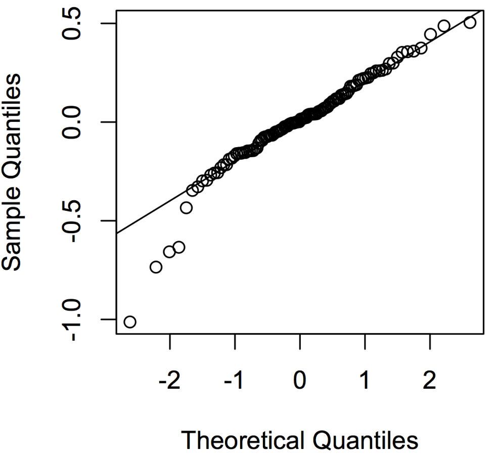
We apply Sparse-LTS , Extended Lasso (Nguyen and Tran 2013), LAD Lasso (Wang et al. 2007), standard Least Squares Lasso estimator (Tibshirani 1996), and ROMP (Chen et al. 2013) to the analysis of yeast genotype and gene expression data. We employ the “yeast” dataset from Brem et al. (2005). The data set concerns $n=112$ F1 segregants from a yeast genetic cross between two strains: BY and RM. For each of these 112 samples, we observe $p=3244$ SNPs (These genotype data are our predictors $x$) and focus on the gene expression of gene GPA1 (our response $y$), which is involved in pheromone response Brem et al. (2005). For both Sparse-LTS-Ada and Sparse LTS considering a total of $|B|=11$ contaminated observations lead to the best predictive performance on the uncontaminated data. In addition, the QQ-plots of the fitted residuals from the various comparison methods indicated heavy left tails (see Figure 4). This suggests that it might be advisable to use robust methods.

We compare the trimmed mean square error (T-MSE) computed from 10-folds cross validation for each method, where for each method we exclude the 11 observations with largest residual absolute error. From Table 3 we can see thatSparse-LTS exhibit the smallest T-MSE.

We conclude by examining the SNPs selected by the methods achieving the lowest T-MSE: Sparse-LTS and LAD Lasso. Out of $p=3244$ SNPs, Sparse-LTS selected 30 SNPs, and LAD Lasso chose 61 SNPs. Table 3 provides a list of the SNPs selected on chromosome 8, which is where gene GPA1 resides. In the dataset, there is a total of 166 SNPs on chromosome 8. From the table we can see that there is some overlap in terms of the selected SNPs across the various methods. Sparse-LTS tends to select a larger number of SNPs on chromosome 8 even though it selects fewer SNPs in total (namely within and beyond chromosome 8). Five of these are very close to GPA1 which is consistent with the fact that GPA1 can directly inhibit the mating signal by binding to its own subunit Stratton et al. (1996).

We analyze a yeast microarray dataset generated by Brem and Kruglyak (2005). The dataset concerns $n=112$ yeast segregants (instances). We focused on $p=126$ genes (variables) belonging to cell-cycle pathway as provided by the KEGG database Kanehisa et al. (2014). For each of these genes we standardize the gene expression data to zero-mean and unit standard deviation. We observed that the expression levels of some genes are clearly not symmetric about their means and might include outliers. For example the histogram of gene ORC3 is presented in Figure 5(a).

For the robust-LL method we set $\beta=0.05$ and for trim-glasso we use $h/n=80\%.$ We use 5-fold-CV to choose the tuning parameters for each method. After $\lambda$ is chosen for each method, we rerun the methods using the full dataset to obtain the final precision matrix estimates.

Figure 5(b) shows the cell-cycle pathway estimated by our proposed method. For comparison the cell-cycle pathway from the KEGG Kanehisa et al. (2014) is provided in Figure 6.

It is important to note that the KEGG graph corresponds to what is currently known about the pathway. It should not be treated as the ground truth. Certain discrepancies between KEGG and estimated graphs may also be caused by inherent limitations in the dataset used for modeling. For instance, some edges in cell-cycle pathway may not be observable from gene expression data. Additionally, the perturbation of cellular systems might not be strong enough to enable accurate inference of some of the links.

glasso tends to estimate more links than the robust methods. We postulate that the lack of robustness might result in inaccurate network reconstruction and the identification of spurious links. Robust methods tend to estimate networks that are more consistent with that from the KEGG ($F_{1}$-score of 0.23 for glasso, 0.37 for t*-lasso, 0.39 for robust-NLL and 0.41 for trim-glasso, where the $F_{1}$ score is the harmonic mean between precision and recall). For instance our approach recovers several characteristics of the KEGG pathway. For instance, genes CDC6 (a key regulator of DNA replication playing important roles in the activation and maintenance of the checkpoint mechanisms coordinating S phase and mitosis) and PDS1 (essential gene for meiotic progression and mitotic cell cycle arrest) are identified as a hub genes, while genes CLB3,BRN1,YCG1 are unconnected to any other genes.

References

- Alfons et al. (2013) Alfons, A., Croux, C., and Gelper, S. (2013), “Sparse least trimmed squares regression for analyzing high-dimensional large data sets,” Ann. Appl. Stat., 7, 226–248.
- Aravkin and Van Leeuwen (2012) Aravkin, A. Y. and Van Leeuwen, T. (2012), “Estimating nuisance parameters in inverse problems,” Inverse Problems, 28, 115016.
- Bannerjee et al. (2008) Bannerjee, O., , Ghaoui, L. E., and d’Aspremont, A. (2008), “Model selection through sparse maximum likelihood estimation for multivariate Gaussian or binary data,” Jour. Mach. Lear. Res., 9, 485–516.
- Beck and Teboulle (2009) Beck, A. and Teboulle, M. (2009), “A fast iterative shrinkage-thresholding algorithm for linear inverse problems,” SIAM Journal on Imaging Sciences, 2, 183–202.
- Boyd and Vandenberghe (2004) Boyd, S. and Vandenberghe, L. (2004), Convex optimization, Cambridge, UK: Cambridge University Press.
- Brem and Kruglyak (2005) Brem, R. B. and Kruglyak, L. (2005), “The landscape of genetic complexity across 5,700 gene expression traits in yeast,” Proceedings of the National Academy of Sciences of the United States of America, 102, 1572–1577.
- Brem et al. (2005) Brem, R. B., Storey, J. D., Whittle, J., and Kruglyak, L. (2005), “Genetic interactions between polymorphisms that affect gene expression in yeast.” Nature, 436, 701–703.
- Bunea (2008) Bunea, F. (2008), “Honest variable selection in linear and logistic regression models via l1 and l1 + l2 penalization,” Electron. J. Stat., 2, 1153–1194.
- Candès et al. (2006) Candès, E., Romberg, J., and Tao, T. (2006), “Stable signal recovery from incomplete and inaccurate measurements,” Communications on Pure and Applied Mathematics, 59, 1207–1223.
- Chen et al. (2013) Chen, Y., Caramanis, C., and Mannor, S. (2013), “Robust High Dimensional Sparse Regression and Matching Pursuit,” The Proceedings of the International Conference on Machine Learning (ICML).
- Cross and Jain (1983) Cross, G. and Jain, A. (1983), “Markov Random Field Texture Models,” IEEE Trans. PAMI, 5, 25–39.
- Daye et al. (2012) Daye, Z., Chen, J., and H., L. (2012), “High-Dimensional Heteroscedastic Regression with an Application to eQTL Data Analysis,” Biometrics, 68, 316–326.
- Finegold and Drton (2011) Finegold, M. and Drton, M. (2011), “Robust graphical modeling of gene networks using classical and alternative T-distributions,” The Annals of Applied Statistics, 5, 1057–1080.
- Friedman et al. (2007) Friedman, J., Hastie, T., and Tibshirani, R. (2007), “Sparse inverse covariance estimation with the graphical Lasso,” Biostatistics.
- Golub and Pereyra (2003) Golub, G. and Pereyra, V. (2003), “Separable nonlinear least squares: the variable projection method and its applications,” Inverse Problems, 19, R1–R26.
- Hassner and Sklansky (1978) Hassner, M. and Sklansky, J. (1978), “Markov Random Field Models of Digitized Image Texture,” in ICPR78, pp. 538–540.
- Ising (1925) Ising, E. (1925), “Beitrag zur Theorie der Ferromagnetismus,” Zeitschrift für Physik, 31, 253–258.
- Kanehisa et al. (2014) Kanehisa, M., Goto, S., Sato, Y., Kawashima, M., Furumichi, M., and Tanabe, M. (2014), “Data, information, knowledge and principle: back to metabolism in KEGG,” Nucleic Acids Res., 42, D199–D205.
- Lauritzen (1996) Lauritzen, S. (1996), Graphical models, Oxford University Press, USA.
- Loh and Wainwright (2015) Loh, P. and Wainwright, M. J. (2015), “Regularized M-estimators with Nonconvexity: Statistical and Algorithmic Theory for Local Optima,” Journal of Machine Learning Research (JMLR), 16, 559–616.
- Loh and Wainwright (2013) Loh, P.-L. and Wainwright, M. J. (2013), “Regularized M-estimators with nonconvexity: Statistical and algorithmic theory for local optima,” in Neur. Info. Proc. Sys. (NIPS), 26.
- Manning and Schutze (1999) Manning, C. D. and Schutze, H. (1999), Foundations of Statistical Natural Language Processing, MIT Press.
- Meinshausen and Bühlmann (2006) Meinshausen, N. and Bühlmann, P. (2006), “High-dimensional graphs and variable selection with the Lasso,” Annals of Statistics, 34, 1436–1462.
- Negahban et al. (2012) Negahban, S., Ravikumar, P., Wainwright, M. J., and Yu, B. (2012), “A unified framework for high-dimensional analysis of M-estimators with decomposable regularizers,” Statistical Science, 27, 538–557.
- Nesterov (2004) Nesterov, Y. (2004), Introductory lectures on convex optimization, vol. 87 of Applied Optimization, Kluwer Academic Publishers, Boston, MA, a basic course.
- Nguyen and Tran (2013) Nguyen, N. H. and Tran, T. D. (2013), “Robust Lasso with missing and grossly corrupted observations,” IEEE Trans. Info. Theory, 59, 2036–2058.
- Oh and Deasy (2014) Oh, J. H. and Deasy, J. O. (2014), “Inference of radio-responsive gene regulatory networks using the graphical lasso algorithm,” BMC Bioinformatics, 15, S5.
- Raskutti et al. (2010) Raskutti, G., Wainwright, M. J., and Yu, B. (2010), “Restricted Eigenvalue Properties for Correlated Gaussian Designs,” Journal of Machine Learning Research (JMLR), 99, 2241–2259.
- Ravikumar et al. (2011) Ravikumar, P., Wainwright, M. J., Raskutti, G., and Yu, B. (2011), “High-dimensional covariance estimation by minimizing -penalized log-determinant divergence,” Electronic Journal of Statistics, 5, 935–980.
- Recht et al. (2010) Recht, B., Fazel, M., and Parrilo, P. A. (2010), “Guaranteed minimum-rank solutions of linear matrix equations via nuclear norm minimization,” SIAM review, 52, 471–501.
- Ripley (1981) Ripley, B. D. (1981), Spatial statistics, New York: Wiley.
- Rockafellar and Wets (2009) Rockafellar, R. T. and Wets, R. J.-B. (2009), Variational analysis, vol. 317, Springer Science & Business Media.
- Rousseeuw (1984) Rousseeuw, P. J. (1984), “Least median of squares regression,” J. Amer. Statist. Assoc., 79, 871–880.
- Stratton et al. (1996) Stratton, H., Zhou, J., Reed, S., and Stone, D. (1996), “The Mating-Specific Galpha Protein of Saccharomyces cerevisiae Downregulates the Mating Signal by a Mechanism That Is Dependent on Pheromone and Independent of Gbetagamma Sequestration,” Molecular and Cellular Biology.
- Sun and Li (2012) Sun, H. and Li, H. (2012), “Robust Gaussian graphical modeling via l1 penalization,” Biometrics, 68, 1197–206.
- Tibshirani and Manning (2014) Tibshirani, J. and Manning, C. D. (2014), “Robust Logistic Regression using Shift Parameters.” in ACL (2), pp. 124–129.
- Tibshirani (1996) Tibshirani, R. (1996), “Regression shrinkage and selection via the lasso,” Journal of the Royal Statistical Society, Series B, 58, 267–288.
- Tu et al. (2016) Tu, N., Aravkin, A., van Leeuwen, T., Lin, T., and Herrmann, F. J. (2016), “Source estimation with surface-related multiples—fast ambiguity-resolved seismic imaging,” Geophysical Journal International, 205, 1492–1511.
- van de Geer and Buhlmann (2009) van de Geer, S. and Buhlmann, P. (2009), “On the conditions used to prove oracle results for the Lasso,” Electronic Journal of Statistics, 3, 1360–1392.
- Vershynin (2012) Vershynin, R. (2012), “Introduction to the non-asymptotic analysis of random matrices,” in Compressed Sensing: Theory and Applications, eds. Eldar, Y. and Kutyniok, G., Cambridge University Press, pp. 210–268, forthcoming.
- Wainwright (2009) Wainwright, M. J. (2009), “Sharp thresholds for high-dimensional and noisy sparsity recovery using -constrained quadratic programming (Lasso),” IEEE Trans. Information Theory, 55, 2183–2202.
- Wang et al. (2007) Wang, H., Li, G., and Jiang, G. (2007), “Robust regression shrinkage and consistent variable selection through the LAD-lasso,” Journal of Business and Economics Statistics, 25, 347–355.
- Woods (1978) Woods, J. (1978), “Markov Image Modeling,” IEEE Transactions on Automatic Control, 23, 846–850.
- Yang and Lozano (2015) Yang, E. and Lozano, A. C. (2015), “Robust Gaussian Graphical Modeling with the Trimmed Graphical Lasso,” in Neur. Info. Proc. Sys. (NIPS), 28.
- Yang and Ravikumar (2013) Yang, E. and Ravikumar, P. (2013), “Dirty Statistical Models,” in Neur. Info. Proc. Sys. (NIPS), 26.
- Yang et al. (2012) Yang, E., Ravikumar, P., Allen, G. I., and Liu, Z. (2012), “Graphical Models via Generalized Linear Models,” in Neur. Info. Proc. Sys. (NIPS), 25.
- Yang et al. (2013) Yang, E., Tewari, A., and Ravikumar, P. (2013), “On Robust Estimation of High Dimensional Generalized Linear Models,” in Inter. Joint Conf. on Artificial Intelligence, 13.
- Yuan and Lin (2007) Yuan, M. and Lin, Y. (2007), “Model selection and estimation in the Gaussian graphical model,” Biometrika, 94, 19–35.
Appendix
Appendix A Proof of Theorem 1
We use the shorthand for local optimal error vector: and where is an arbitrary local optimum of -estimator of (4). Our proof mainly uses the fact that is a local minimum of (4) satisfying
This inequality comes from the first order stationary condition (see Loh and Wainwright (2015) for details) in terms of only fixing at . In order to provide the complete proof of the theorem, we need to define the set of notations on the model space, perturbation space and corresponding projections following Negahban et al. (2012). The sparse LTS (3) is a typical example of (4), and such notations can be naturally defined based on the true support set . In this proof, we specifically focus on the case with for notational simplicity, but statements here can be seamlessly extendible for the general regularizer and the appropriately defined model/perturbation spaces.
If we take above, we have