Bounds and extremal domains for Robin eigenvalues with negative boundary parameterThanks: This research was partially supported by FCT (Portugal) through project PTDC/MAT-CAL/4334/2014. The first author was also supported through the program “Investigador FCT” with reference IF/00177/2013. The third author was also supported by the project RVO61389005 and the GACR grant No. 14-06818S
Abstract.
We present some new bounds for the first Robin eigenvalue with a negative boundary parameter. These include the constant volume problem, where the bounds are based on the shrinking coordinate method, and a proof that in the fixed perimeter case the disk maximises the first eigenvalue for all values of the parameter. This is in contrast with what happens in the constant area problem, where the disk is the maximiser only for small values of the boundary parameter. We also present sharp upper and lower bounds for the first eigenvalue of the ball and spherical shells.
These results are complemented by the numerical optimisation of the first four and two eigenvalues in and dimensions, respectively, and an evaluation of the quality of the upper bounds obtained. We also study the bifurcations from the ball as the boundary parameter becomes large (negative).
- Keywords:
eigenvalue optimisation, Robin Laplacian, negative boundary parameter, Bareket’s conjecture
- MSC (2010):
58J50, 35P15
1. Introduction
The study of extremal eigenvalues of the Laplace operator which had its origin in Lord Rayleigh’s book The Theory of Sound [33] has by now been a continuous active topic of research among mathematicians and physicists for nearly one century and a half. In the case of Dirichlet and Neumann boundary conditions it has been known since the ’s and the ’s, respectively, that the ball optimises the first eigenvalue among domains with fixed volume, being a minimiser in the first case and a maximiser in the second [15, 26, 27, 35, 36]. In the case of Dirichlet boundary conditions this implies that the second eigenvalue is optimised by two equal balls [27], while for the Neumann problem it is only known that this provides a bound for planar simply connected domains [22].
Recent numerical work has shown that, with some rare exceptions, notably that of the Dirichlet eigenvalue in dimension which is conjectured to be optimised by the ball, one cannot expect extremal domains in the mid-frequency range to be defined explicitly in terms of known functions [6, 5, 30]. For planar domains with fixed area, it has been shown that the disk cannot be a minimiser for eigenvalues higher than the third [10]. On the other hand, this has prompted the study of what happens in the high-frequency limit as the order of the eigenvalue goes to infinity, where there is again some structure. In particular, it was shown by Dorin Bucur and the second author of the present paper that for planar domains with fixed perimeter extremal domains converge to the disk [12]. In the case of fixed measure, the first two authors of the present paper showed that minimisers of the Dirichlet problem within the class of rectangles converge to the square [7] and, moreover, it has been shown that convergence to the disk in the general case is equivalent to the well-known Pólya conjecture [13].
In this paper we are interested in extremal domains for eigenvalues of the Robin Laplacian, that is,
| (1.1) |
where is a bounded domain in with outer unit normal and the boundary parameter is a real constant.
In the case of fixed measure of and positive boundary parameter, it was only in that it was proven that the disk is still the extremal domain in two dimensions [11], while the extension of this result to higher dimensions had to wait until [14]. The corresponding result for the second eigenvalue was obtained in [25], with two equal balls being the minimal domain, again matching the Dirichlet result. However, due to the presence of a boundary parameter in the Robin problem, the behaviour for higher eigenvalues will be, in principle, more complex as may be seen from the numerical results in [8]. In particular, for a given fixed volume and small positive values of the boundary parameter it is conjectured in that paper that the eigenvalue will in fact be minimised by equal balls, but that this will not be the case for larger values of the parameter. This switching between extremal domains as the parameter changes was recently shown by the second and third authors of the present paper to also play a role for negative values of the parameter, even in the case of the first eigenvalue [18]. More precisely, while it was shown that in two dimensions the disk remains an extremal domain for small (negative) values of the parameter (now a maximiser), thus proving the long standing Bareket’s conjecture [9] in that case, it was also shown that for larger (negative) values of the parameter it cannot remain the optimiser. This provides the first known example where the extremal domain for the lowest eigenvalue of the Laplace operator is not a ball.
The proof that the disk cannot remain the optimiser for all values of the boundary parameter is based on the comparison between the asymptotic behaviour of the eigenvalues of disks and annuli as the boundary parameter goes to minus infinity, and carries over to higher dimensions. More precisely, while the asymptotic behaviour of a ball with radius in is given by
| (1.2) |
that of a spherical shell with radii is given by
| (1.3) |
We thus see that, if is larger than , must become larger than for sufficiently large negative .
On the other hand, let us recall that Bareket has proved her conjecture already in [9] for a class of “nearly circular domains” and Ferone, Nitsch and Trombetti [16] have shown recently that it holds within the “class of Lipschitz sets which are ‘close’ to a ball in a Hausdorff metric sense”. Our proof from [18] for small (negative) values of the parameter differs from immediate results based on a simple perturbation argument (see, e.g., [28, Sec. 2.3]) in that the smallness of is shown to depend on the area of only (cf. [18, Rem. 2]).
In this paper we shall complete these results in the following directions. We shall begin by providing a new upper bound for the first eigenvalue under a fixed volume restriction.
Theorem 1.
Let . Let be a strictly star-shaped bounded domain in with Lipschitz boundary and let be the ball of the same volume. Then
| (1.4) |
where is a geometric quantity related to the support function of defined by (3.3).
The proof of Theorem 1 is done using an approach based on shrinking coordinates which were introduced in [32] in the two-dimensional case and then extended to higher dimensions in [17].
We then consider the case of fixed perimeter in dimension two for which we show that, in contrast with the fixed area problem, the disk is now the maximiser for all negative values of the boundary parameter .
Theorem 2.
Let . For bounded planar domains of class , we have
where is a disk with the same perimeter as .
The proof of Theorem 2 is based on an intermediate result from [18] established with help of parallel coordinates.
Complementing the above results, we provide sharp bounds for the first eigenvalue of the ball in any dimensions.
Theorem 3.
Let denote the -dimensional ball of radius and denote by its first Robin eigenvalue. Then we have
for all negative .
Note that this result actually states that the first eigenvalue of the ball is smaller than the first two terms in the asymptotic expansion (1.2) for all negative values of the boundary parameter . Furthermore, it is not difficult to check that the lower bound satisfies the same two-term asymptotics, with the next term being of order . We also see that, for fixed , goes to with as goes to zero. On the other hand, it follows from the upper bound that, whenever is negative, does not go to as (see also Remark 2 below).
We also establish sharp lower and upper bounds for the first Robin eigenvalue in -dimensional spherical shells, which, as explained above, we conjecture are the extremal sets for large negative .
Theorem 4.
Let denote the -dimensional spherical shell with inner and outer radii given by and , respectively, and denote by its first Robin eigenvalue. Then we have
| (1.5) |
for all negative .
Here the upper bound is optimal up to the second order as , cf. (1.3), and we see that, as in the case of the ball, the eigenvalue is bounded by the first two terms in the asymptotics. The lower bound follows the first-order asymptotics only.
Finally, we perform a numerical study to obtain insight into the structure that is to be expected for this problem. In particular, our results support the conjecture that the first eigenvalue is also maximised by the ball for small negative values of in three dimensions and that both in this case and in the plane shells with varying (increasing) radii become the extremal domain as becomes more negative. We also study the optimisation of higher eigenvalues. Based on these numerical simulations, we formulate some conjectures at the end of the paper.
2. The first eigenvalue of balls and shells
Let be a bounded domain in () with Lipschitz boundary and . As usual, we understand (1.1) as a spectral problem for the self-adjoint operator in the Hilbert space associated with the closed quadratic form
| (2.1) |
The lowest point in the spectrum of can be characterised by the variational formula
| (2.2) |
Since the embedding is compact, we know that is indeed a discrete eigenvalue and the infimum is achieved by a function .
Using a constant test function in (2.2), we get
| (2.3) |
Here denotes the -dimensional Lebesgue measure in the denominator and the -dimensional Hausdorff measure in the numerator. It follows that is negative whenever .
Now let be a -dimensional ball of radius . By the rotational symmetry and regularity, we deduce from (2.2)
| (2.4) |
We know that is simple and that the infimum in (2.4) is achieved by a smooth positive function satisfying
| (2.5) |
In fact, if , we have an explicit solution
| (2.6) |
where is a modified Bessel function [1, Sec. 9.6] and is the smallest non-negative root of the equation
| (2.7) |
Using the identity (cf. [1, Sec. 9.6.26])
| (2.8) |
we see that (2.7) is equivalent to
| (2.9) |
Lemma 1.
Proof.
2.1. An upper bound for
| (2.11) |
we obtain the bound
| (2.12) |
with
| (2.13) |
Hence the upper bound of Theorem 3 follows provided that (recall that is negative)
| (2.14) |
To prove (2.14), we first notice the identity
| (2.15) |
which can be established by an integration of parts. Second, we have
| (2.16) |
because for all with . As a consequence of (2.15) and (2.16), we have
| (2.17) |
which proves (2.14) and thus concludes the proof of the upper bound of Theorem 3. ∎
2.2. A lower bound for
To obtain the lower bound in Theorem 3 we shall use a different strategy based directly on equation (2.9) and properties of quotients of Bessel functions. A similar approach may also be used as an alternative way of establishing the upper bound in the previous section.
From [4] we have
| (2.18) |
where justification that strict inequality holds may be found in [34]. Applying this to equation (2.9) for negative yields
from which it follows that
| (2.19) |
Due to the upper bound proved in the previous section we know that
and thus
from which it follows that the left-hand side of (2.19) is positive. We may thus square both sides of (2.19) to obtain
This implies both a lower and an upper bounds for and while the lower bound is trivial, the upper bound yields the desired lower bound for the eigenvalue .
2.3. Monotonicity for balls
In this subsection we give a proof of the following monotonicity result.
Theorem 5.
Let be a ball of radius . If , then
We remark that a non-strict monotonicity of the first Robin eigenvalue for certain domains (including balls) has been obtained in [19] (see also [20] and [21]). Since our proof of Theorem 5 employs different ideas and yields the strict monotonicity, we have decided to present it here.
For simplicity, throughout this subsection we set . We also write to stress the dependence of the eigenfunction on the radius.
Our proof of Theorem 5 is based on the following formula for the derivative of with respect to .
Lemma 2.
We have
| (2.20) |
Proof.
By the unitary transform , we see that is the lowest eigenvalue of the operator in the -independent Hilbert space associated with the quadratic form
Since forms a holomorphic family in (cf. [24, Thm. VII.4.8]) and is simple, and the associated eigenprojection are holomorphic functions of . In particular, the eigenfunction of associated with can be chosen to depend continuously on in the topology of . Now, the weak formulation of the eigenvalue problem for reads
| (2.21) |
for every , where and denote the sesquilinear form associated with and the inner product in , respectively. Differentiating (2.21) with respect to (which is justified by the holomorphic properties of and ) and employing (2.21) in the resulting identity, we conclude with
This formula coincides with (2.20) through the unitary identification . ∎
The derivative (2.20) is clearly negative whenever is positive. At the same time, the derivative (2.20) is zero for the Neumann case . If is negative, the numerator of (2.20) consists of a negative and a positive term, so the sign of the derivative is not obvious in this case. Our strategy to prove Theorem 5 is to show that the derivative is in fact positive whenever is negative.
By employing (2.4), where the infimum is actually achieved for , we can rewrite (2.20) as follows
| (2.22) |
Note that the sign of the numerator is still unclear because whenever , cf. (2.3). However, expression (2.22) is convenient because of the following lemma.
Lemma 3.
Let . Then
| (2.23) |
Proof.
2.4. Bounds for
In this subsection, we establish Theorem 4 dealing with -dimensional spherical shells.
Proof of Theorem 4.
Now we have the variational characterisation
| (2.25) |
To prove the lower bound, let be a positive minimiser of (2.25). Given any Lipschitz-continuous function such that
we write
Denoting by the numerator of the right-hand side of (2.25), we therefore have
| (2.26) | ||||
where
| (2.27) |
with
We remark that the second inequality in (2.26) is strict provided that the function is not constant. In this case, we deduce from (2.26)
| (2.28) |
The function can be understood as a sort of test function.
Choosing now
| (2.29) |
we obtain
The function is clearly non-constant and we claim that it is minimised at . To see the latter, we write
where the last two terms are individually non-negative because and is negative. Consequently, with the special choice (2.29),
| (2.30) |
We now turn to the upper bound. In the variational characterisation (2.25), we again use the test function (2.11) with being replaced by now. It leads to the upper bound
| (2.31) |
with
| (2.32) |
Since , where is defined in (2.13), we have
| (2.33) |
Here the last bound coincides with the upper bound (2.12) for balls. Using (2.14), we thus obtain the upper bound of Theorem 4. ∎
Remark 1.
Adapting the idea of the lower-part proof above to balls, we obtain , where is defined as in (2.27) with and and is any Lipschitz-continuous (test) function such that
Taking , we then arrive at the lower bound
| (2.34) |
This is not as good as the lower bound of Theorem 3, but, on the other hand, it is much simpler.
2.5. The Robin problem in dimension
Finally, let us make a few comments on problem (1.1) when is an interval. While the one-dimensional situation is formally excluded from this paper, our main results still hold in that case. In fact, the case of is simpler in the sense that it can be reduced to a single transcendental equation.
To be more specific, without loss of generality, let us assume now that is a one-dimensional ball of radius centred at the origin, i.e. . From (2.3) we know that is negative as long as . By solving the differential equation in (1.1) in terms of exponentials, subjecting the general solution to the boundary conditions at and employing the fact that the corresponding eigenfunction cannot change sign, we obtain that , where is the smallest positive solution of
| (2.35) |
First of all, we study the asymptotic regime when the boundary parameter goes to minus infinity.
Proposition 1.
We have the asymptotics
| (2.36) |
Proof.
It follows from (2.3) that as . Since the right-hand side of (2.35) tends to as , we immediately obtain that as . Let us put . Subtracting from both sides of (2.35), we now rewrite (2.35) as follows
Since as , the identity asymptotically behaves as
Multiplying this asymptotic identity by and taking the limit , we conclude with
which completes the proof of the proposition. ∎
The proposition represents an improvement upon (1.2) when . Let us emphasise that the asymptotics does not enable one to extend the disproval of Bareket’s conjecture from [18] to the one-dimensional situation. When , the analogue of the annulus of positive radii is the disconnected set . Since, with and the one-dimensional ball of radius such that satisfy , it actually follows from Proposition 1 that
| (2.37) |
for all sufficiently large negative . As a matter of fact, assuming the volume constraint , inequality (2.37) does hold for all negative ; this follows from the following monotonicity result (cf. Theorem 5).
Proposition 2.
If , then
Proof.
The proof of Theorem 5 does not seem to entirely extend to . Anyway, in the present one-dimensional situation, the monotonicity result can be deduced directly from (2.35). Let us set
Computing the partial derivatives,
we conclude from the implicit-function theorem that the derivative of with respect to is negative. Consequently,
which completes the proof of the proposition. ∎
We complement Proposition 2 by the asymptotic behaviour of the first Robin eigenvalue in shrinking and expanding intervals.
Proposition 3.
If , then
Proof.
Remark 2.
It is remarkable that does not converge to zero as , which is the lowest point in the spectrum of the “free” Laplacian . Consequently, cannot converge to in a norm-resolvent sense as . This is still true in higher dimensions, as may be seen from the upper bound in Theorem 3.
For later purposes, we apply Proposition 3 to the behaviour of the first Robin eigenvalue in long thin rectangles.
Corollary 1.
Let be a rectangle of half-sides and . If , then
Proof.
By separation of variables, we have
The asymptotic behaviour is then a direct consequence of Proposition 3. ∎
3. Fixed volume: upper bounds
In this section we give a proof of Theorem 1.
3.1. Star-shaped geometries
Following [17], we assume that is star-shaped with respect to a point , i.e., for each point the segment joining with lies in and is transversal to at the point . By Rademacher’s theorem, the outward unit normal vector field can be uniquely defined almost everywhere on . At those points for which is uniquely defined, we introduce the support function
| (3.1) |
where the dot denotes the standard scalar product in .
We say that is strictly star-shaped with respect to the point if is star-shaped with respect to and the support function is uniformly positive, i.e.,
| (3.2) |
In this case, we shall denote by the set of points with respect to which is strictly star-shaped, and define the following intrinsic quantity of the domain
| (3.3) |
where denotes the surface measure of . We refer to [17] for evaluation of the quantity for certain special domains.
3.2. Shrinking coordinates
Given a point with respect to which is strictly star-shaped, we parameterise by means of the mapping
| (3.4) |
It has been shown in [17] that indeed induces a diffeomorphism, so that can be identified with the Riemannian manifold with the induced metric , for which, in particular,
| (3.5) |
Here , denotes the metric tensor of (as a submanifold of ) and are the coefficients of the inverse metric . Consequently, the volume element of the manifold is decoupled as follows:
| (3.6) |
In contrast with (3.3), the integral of the support function is actually independent of . Indeed, recalling (3.6), we have the following identity for the Lebesgue measure of
| (3.7) |
For the -dimensional Hausdorff measure of , we have .
The following proposition provides a lower bound to the geometric quantity (3.3).
Proposition 4.
Let be a bounded strictly star-shaped domain in with Lipschitz boundary . Then
| (3.8) |
where is a ball of the same volume as . Here the second equality is attained for is larger than two if, and only if, , and it holds for any disk when is two; the first inequality is attained for any ball.
Proof.
By the Schwarz inequality,
| (3.9) |
for any . Recalling (3.7) and minimising over , we get the first inequality of (3.8). The second estimate in (3.8) follows by the isoperimetric inequality, which is known to be optimal if, and only if, . Finally, it is easy to see that
| (3.10) |
for any ball of radius . ∎
Using the identification of with , we introduce the unitary transform from the Hilbert space to by . Then
| (3.11) | ||||
where the Einstein summation convention is assumed in the central line, with for using some local parameterisation of and .
3.3. Proof of Theorem 1
With help of the unitary transform above, we choose in (2.2) a test function , where depends on the radial variable only, i.e. with any smooth function . Using (3.11), (3.6) and (3.5), we thus obtain
| (3.12) |
for any smooth and every . Minimising over and recalling (3.3) and (3.7), we arrive at the bound
| (3.13) |
for any smooth .
Now, let an open ball of the same volume as , i.e. . Employing the fact that the eigenfunction of corresponding to the lowest eigenvalue is radially symmetric, we have the equality
| (3.14) |
with some smooth function .
3.4. Comments on Theorem 1
3.4.1. Theorem 1 does not prove Bareket’s conjecture
By Proposition 4,
| (3.15) |
(recall that is non-positive for any , cf. (2.3)). However, since Proposition 4 also implies
| (3.16) |
where the second inequality follows from the isoperimetric inequality, the bound (1.4) together with these estimates does not seem to give anything useful as regards Bareket’s conjecture (that requires ).
3.4.2. Bound (1.4) is not optimal in the limit
3.4.3. Bound (1.4) is optimal in the limit
Indeed, by analytic perturbation theory (see, e.g., [28]),
| (3.19) |
Consequently, (1.4) implies
| (3.20) |
and it remains to recall that . Moreover, since
| (3.21) |
the argument also implies that (1.4) yields the validity of for all the negative which have sufficiently small (with the smallness depending on ).
3.4.4. Bound (1.4) is optimal for long thin rectangles
Let be a rectangle of half-sides and and let us compare the upper bound of Theorem 1 with the actual eigenvalue of the rectangle. We are interested in the regime when and , while keeping the area of the rectangle fixed, say . All the asymptotic formulae below in this subsection are with respect to this limit.
The geometric quantity was computed in [17] for various domains including rectangular parallelepipeds and ellipsoids. In particular, [17, Ex. 1] and [17, Ex. 2] (see also (3.10)) respectively yield
where is the disk of the same area as , i.e. the radius of equals . (Note that is independent of if .)
We have and . Consequently, the ratio behaves as and the same decay rate holds for from (1.4). Using (3.19), we therefore have
Consequently, the upper bound for given by Theorem 1 reads
| (3.22) |
At the same time, Corollary 1 implies the exact asymptotics
| (3.23) |
We see that the leading orders of (3.22) and (3.23) coincide.
4. Fixed perimeter: the disk maximises the first eigenvalue
In this section we restrict to . Moreover, we assume that the bounded domain is of class . Then the boundary will, in general, be composed of a finite union of -smooth Jordan curves , , where is the outer boundary i.e. lies in the interior of . If , then is simply connected and .
We denote by and the perimeter and outer perimeter of , respectively, where stands for the -dimensional Hausdorff measure. By the isoperimetric inequality, we have , where denotes the area of . Here stands for the -dimensional Lebesgue measure.
Under our regularity assumptions, the operator domain consists of functions which satisfy the Robin boundary conditions of (1.1) in the sense of traces and the boundary value problem (1.1) can be thus considered in a classical setting.
4.1. An upper bound from [18]
As in [18], the main ingredient in our proof of Theorem 2 is the method of parallel coordinates that was originally used by Payne and Weinberger [31] in the Dirichlet case (which formally corresponds to in the present setting). It consists in choosing a test function in (2.2) whose level lines are parallel to the boundary of . As a matter of fact, since is non-positive, it is possible to base the coordinates on the outer component only. The result of this approach is the following theorem established in [18].
Theorem 6 ([18]).
Let . For any bounded planar domain of class ,
where is the first eigenvalue of the Laplacian in the annulus with radii
| (4.1) |
subject to the Robin boundary condition with on the outer circle and the Neumann boundary condition on the inner circle.
We note that has the same area as , i.e. . Using the rotational symmetry and polar coordinates, the variational characterisation of the Robin-Neumann eigenvalue reads
| (4.2) |
4.2. Proof of Theorem 2
The following upper bound represents a crucial step in our proof of Theorem 2.
Proposition 5.
Let . For any , we have
where denotes the disk of radius .
Proof.
By symmetry, is the smallest solution of the one-dimensional boundary-value problem
| (4.3) |
The associated eigenfunction can be chosen to be positive and normalised to one in . Using as a test function in (4.2) and integrating by parts, we obtain
| (4.4) |
At the same time, using the differential equation in (2.5), we have
for all , where the inequality follows from the fact that is non-positive, cf. (2.3). Hence, is non-decreasing and the proposition follows as a consequence of (4.4). ∎
Clearly the area of is greater than the area of . On the other hand, the perimeter of is less than the perimeter of , indeed
the outer perimeter of . Hence, Theorem 6 together with Proposition 5 immediately implies Theorem 2 for simply connected domains , when .
To conclude the proof of Theorem 2 in the general case of possibly multiply connected domains, we recall the monotonicity result of Theorem 5. Consequently,
| (4.5) |
for all (the statement is trivial for ), where is chosen in such a way that has the same perimeter as . Summing up, Theorem 2 is proved as a consequence of Theorem 6, Proposition 5 and (4.5). ∎
4.3. Comments on Theorem 2
5. Numerical results
5.1. Extremal domains
In this section we present the main results that we gathered for the optimisation of Robin eigenvalues with negative parameter. In all the numerical simulations we considered domains with unit area and the eigenvalues were calculated using the method of fundamental solutions [2, 3]. The maximisation of Robin eigenvalues was solved by a gradient type method involving Hadamard shape derivatives which allows to minimise a sequence of functionals
for a gradually increasing sequence of penalty parameters .
We assume that is simple, is an associated normalised real-valued eigenfunction and use the notation , where is the identity and is a given deformation field. The Hadamard shape derivative for simple Robin eigenvalues is given by (see, e.g., [23, Ex. 3.5])
where is the mean curvature of and is the tangential component of the gradient of . We note that special variants of this formula for homothetic deformations of balls can be found in Section 2.3.
In the optimisation of each of the eigenvalues we considered the case of connected and disconnected domains with up to connected components. In the latter the optimisation was performed at all the connected components. At the end, the optimal eigenvalue was the maximal eigenvalue obtained from all the cases.
Figure 1-left shows the results for the maximisation of the first Robin eigenvalue as a function of the Robin parameter . In blue we plot the first eigenvalue of the disk of unit area while similar results for the maximal eigenvalue among annuli are shown in red. We will denote by the maximiser of the -th eigenvalue in the class of the annuli of unit area, for a given Robin parameter . Although the two graphs are quite close, it does turn out that while the disk is the (unique) global maximiser for with , there is a transition at where this role is then taken by . For we have non-uniqueness of the maximiser. In the right plot of the same figure we show the difference , for the region .
(a)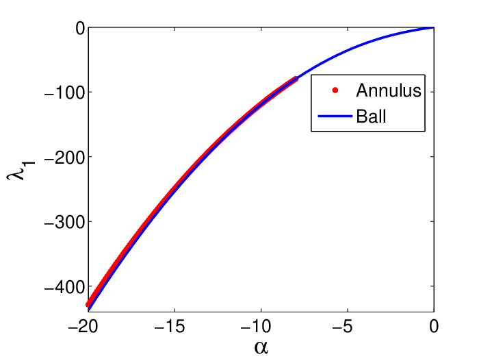 (b)
(b)
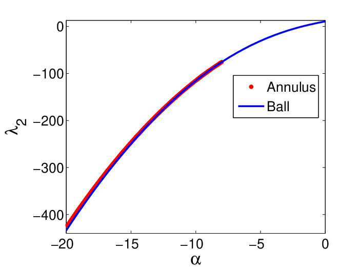
In Figure 2 we plot the maximal second Robin eigenvalue. Again, the maximiser is an annulus for and the ball for .
In Figure 3 we plot the inner radius of the optimal annuli and , as a function of . We observe that in both cases the inner radius decreases with the decrease in .

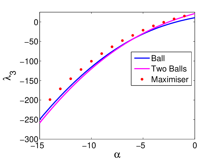
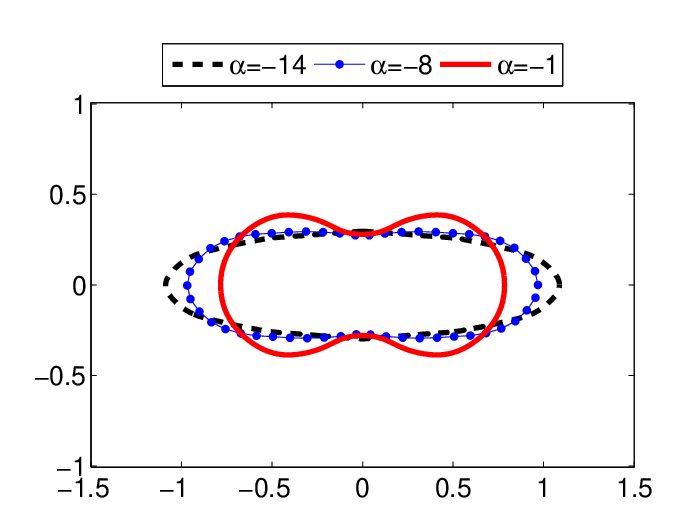
In Figure 4 we plot the optimal third eigenvalue for some Robin parameters . For a comparison, we include also the third eigenvalue of the ball and of the union of two balls of the same area. In this case, our numerical results suggest that the maximisers are always connected, for an arbitrary . Moreover, these maximisers degenerate to two balls for , which is the conjectured maximiser in the case of Neumann boundary conditions – see [22] where it is shown that the third eigenvalue of simply connected domains with Neumann boundary conditions never exceeds this value. In the right plot of the same figure we show the maximisers for .
In Figure 5 we show the numerical maximisers obtained for , .

We shall now present the numerical results obtained for three-dimensional domains. We denote by the maximiser of the -th eigenvalue within the class of spherical shells of unit volume, for a given value of the Robin parameter . In Figure 6 we plot the maximal first and second Robin eigenvalues. In this case, the ball is the maximiser of , , for , while for the maximiser becomes , where the values of obtained numerically are and . We also considered the maximisation of the first Robin eigenvalue among domains with a given surface area. In this case our numerical results suggest that the ball is always the maximiser.
(a)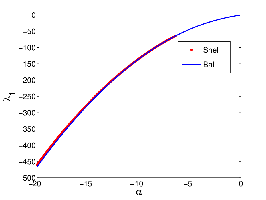 (b)
(b)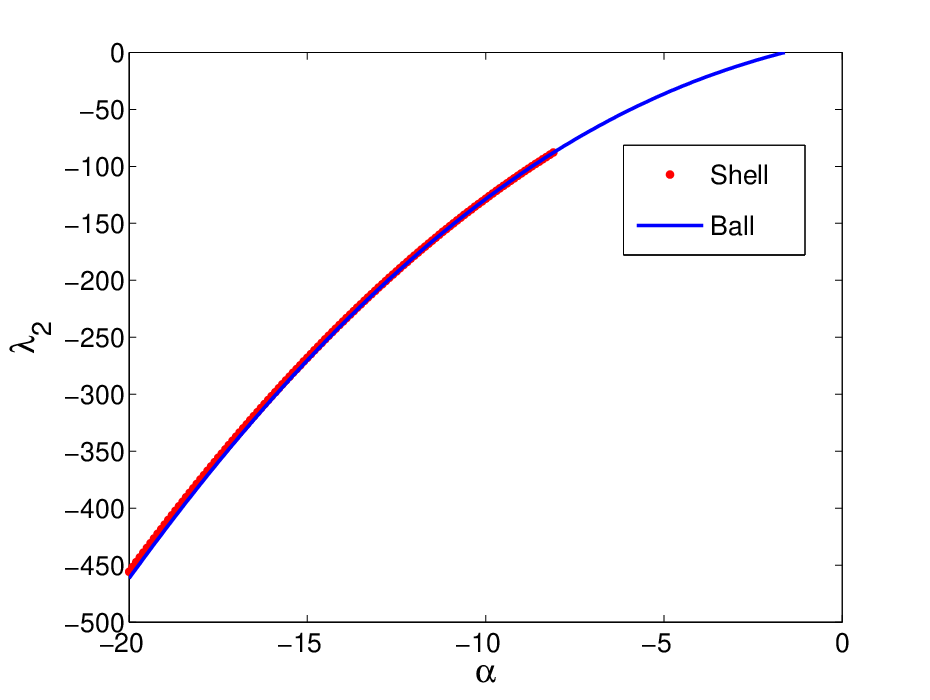
Finally, and in order to understand the behaviour of the bifurcation point where the switching between balls and shells takes place, we analysed numerically the equations determining the eigenvalues of these two domains where we now take the dimension variable to change continuously between and . From Figure 7 we see that both the critical value where the bifurcation occurs and the corresponding value of the inner radius increase as the dimension increases.
(a) (b)
(b)
5.2. Evaluation of upper bounds
In this section we test the bounds provided by Theorems 1, 2 and 6. For a given domain we define the percentage errors associated with these bounds respectively by
In order to illustrate the accuracy of the bounds we shall consider ellipses, ellipsoids, rectangles and parallelepipeds.
Figure 8 shows the percentage errors , and obtained in the class of ellipses as a function of the eccentricity, for .


Figure 9 shows the percentage errors obtained in the class of the rectangles for , as a function of , where is the length of the largest side of the rectangle. Note that the percentage errors of the bound of Theorem 1 converge to zero, as converge to 1. This means that besides the balls, the bound of Theorem 1 gives also equality asymptotically for thin rectangles. This numerical observation is consistent with the analysis made in Section 3.4.4. Indeed, from (3.22) and (3.23) there it follows that as , while keeping the area of the rectangle equal to one.

In the three-dimensional case, for a given ellipsoid with semi-axes lengths , we define the quantities and , for which we have . In Figure 10 we plot the percentage errors obtained for ellipsoids, as a function of and , for .


Finally, we tested the bound of Theorem 1 for parallelepipeds. We will assume that each parallelepiped has length sides and define the quantities and . Figure 11 shows the percentage errors obtained in the class of parallelepipeds, as a function of and .


5.3. Conjectures
The numerical simulations carried out support the conjecture, already formulated in [18], that there is a switch betwen maximisers, with spherical shells becoming the maximisers for sufficiently large (negative) values of the parameter. We may now be more precise.
Conjecture 1.
There exists a negative value of , say , such that the first eigenvalue of problem (1.1) is maximised by the ball among all the domains with equal volume, for .
For smaller than , the maximiser becomes a spherical shell whose radii increase as decreases.
The actual values of and the radii of the shells depend on the dimension and the volume only.
In two dimensions, imposing the extra condition that the domain is simply connected will strongly restrict maximisers.
Conjecture 2.
In two dimensions the disk maximises the first eigenvalue of problem (1.1) for negative , among all simply connected domains with the same area.
Simply connectedness is is clearly not enough to restrict maximisers to balls in higher dimensions and it becomes thus necessary to impose stronger conditions. Although there are other possibilities such as requiring that the boundary be connected, here we just explored the case where domains are convex.
Conjecture 3.
The ball maximises the first eigenvalue of problem (1.1) for negative , among all convex domains with the same volume.
Finally, our results support the conjecture that Theorem 2 may be extended to any dimension.
Conjecture 4.
The ball maximises the first eigenvalue of problem (1.1) for negative , among all domains of equal surface area.
References
- [1] M. S. Abramowitz and I. A. Stegun, eds., Handbook of mathematical functions, Dover, New York, 1965.
- [2] C. J. S. Alves and P. R. S. Antunes, The method of fundamental solutions applied to the calculation of eigenfrequencies and eigenmodes of 2D simply connected shapes, Comput. Mater. Continua 2 (2005), 251–266.
- [3] by same author, The method of fundamental solutions applied to some inverse eigenproblems, SIAM J. Sci. Comp. 35 (2013), A1689–A1708.
- [4] D. E. Amos, Computation of modified Bessel functions and their ratios, Math. Comp. 28 (1974), 239–251.
- [5] P. R. S. Antunes and P. Freitas, Optimisation of eigenvalues of the Dirichlet Laplacian with a surface area restriction, Appl. Math. Optimiz. 73 (2016), 313–328.
- [6] by same author, Numerical optimization of low eigenvalues of the Dirichlet and Neumann Laplacians, J. Opt. Theory Appl. 154 (2012), 235–257.
- [7] by same author, Optimal spectral rectangles and lattice ellipses, Proc. R. Soc. London, Ser. A 469 (2013), 20120492.
- [8] P. R. S. Antunes, P. Freitas, and J. B. Kennedy, Asymptotic behaviour and numerical approximation of optimal eigenvalues of the Robin Laplacian, ESAIM: Control, Optimisation and Calculus of Variations 19 (2013), 438–459.
- [9] M. Bareket, On an isoperimetric inequality for the first eigenvalue of a boundary value problem, SIAM J. Math. Anal. 8 (1977), 280–287.
- [10] A. Berger, The eigenvalues of the Laplacian with Dirichlet boundary condition in are almost never minimized by disks, Ann. Glob. Anal. Geom. 47 (2015), 285–304.
- [11] M.-H. Bossel, Membranes élastiquement liées: Extension du théoréme de Rayleigh-Faber-Krahn et de l’inégalité de Cheeger, C. R. Acad. Sci. Paris Sér. I Math. 302 (1986), 47–50.
- [12] D. Bucur and P. Freitas, Asymptotic behaviour of optimal spectral planar domains with fixed perimeter, J. Math. Phys. 54 (2013), 053504.
- [13] B. Colbois and A. El Soufi, Extremal eigenvalues of the Laplacian on Euclidean domains and closed surfaces, Math. Z. 278 (2014), 529–546.
- [14] D. Daners, A Faber-Krahn inequality for Robin problems in any space dimension, Math. Ann. 335 (2006), 767–785.
- [15] G. Faber, Beweis dass unter allen homogenen Membranen von gleicher Fläche und gleicher Spannung die kreisförmige den tiefsten Grundton gibt, Sitz. bayer. Akad. Wiss. (1923), 169–172.
- [16] V. Ferone, C. Nitsch, and C. Trombetti, On a conjectured reversed Faber-Krahn inequality for a Steklov-type Laplacian eigenvalue, Commun. Pure Appl. Anal. 14 (2015), 63–81.
- [17] P. Freitas and D. Krejčiřík, A sharp upper bound for the first Dirichlet eigenvalue and the growth of the isoperimetric constant of convex domains, Proc. Amer. Math. Soc. 136 (2008), 2997–3006.
- [18] P. Freitas and D. Krejčiřík, The first Robin eigenvalue with negative boundary parameter, Adv. Math. 280 (2015), 322–339.
- [19] T. Giorgi and R. G. Smits, Monotonicity results for the principal eigenvalue of the generalized Robin problem, Illinois J. Math. 49 (2005), 1133–1143.
- [20] by same author, Eigenvalue estimates and critical temperature in zero fields for enhanced surface superconductivity, Z. angew. Math. Phys. 58 (2007), 1224–245.
- [21] by same author, Bounds and monotonicity for the generalized Robin problem, Z. angew. Math. Phys. 59 (2008), 600–618.
- [22] A. Girouard, N. Nadirashvili, and I. Polterovich, Maximization of the second positive Neumann eigenvalue for planar domains, J. Diff. Geometry 83 (2009), 637–662.
- [23] D. Henry, Perturbation of the boundary in boundary-value problems of partial differential equations, Cambridge University Press, New York, 2005.
- [24] T. Kato, Perturbation theory for linear operators, Springer-Verlag, Berlin, 1966.
- [25] J. B. Kennedy, An isoperimetric inequality for the second eigenvalue of the Laplacian with Robin boundary conditions, Proc. Amer. Math. Soc. 137 (2009), 627–633.
- [26] E. Krahn, Über eine von Rayleigh formulierte Minimaleigenschaft des Kreises, Math. Ann. 94 (1924), 97–100.
- [27] by same author, Über Minimaleigenschaft der Kugel in drei und mehr Dimensionen, Acta Comm. Univ. Tartu (Dorpat) A 9 (1926), 1–44.
- [28] A. A. Lacey, J. R. Ockendon, and J. Sabina, Multidimensional reaction diffusion equations with nonlinear boundary conditions, SIAM J. Appl. Math. (1998), 1622–1647.
- [29] M. Levitin and L. Parnovski, On the principal eigenvalue of a Robin problem with a large parameter, Math. Nachr. 281 (2008), 272–281.
- [30] E. Oudet, Numerical minimization of eigenmodes of a membrane with respect to the domain, ESAIM Control Optim. Calc. Var. 10 (2004), 315–330.
- [31] L. E. Payne and H. F. Weinberger, Some isoperimetric inequalities for membrane frequencies and torsional rigidity, J. Math. Anal. Appl. 2 (1961), 210–216.
- [32] G. Pólya and G. Szegö, Isoperimetric inequalities in mathematical physics, Ann. of Math. Studies, no. 27, Princeton University Press, Princeton, 1951.
- [33] J. W. S. Rayleigh, The theory of sound, Macmillan, London, 1877, 1st edition (reprinted: Dover, New York (1945)).
- [34] J. Segura, Bounds for ratios of modified Bessel functions and associated Turán-type inequalities, J. Math. Anal. Appl. 374 (2011), 516–528.
- [35] G. Szegö, Inequalities for certain eigenvalues of a membrane of given area, J. Rational Mech. Anal. 3 (1954), 343–356.
- [36] H. F. Weinberger, An isoperimetric inequality for the -dimensional free membrane problem, J. Rational Mech. Anal. 5 (1956), 633–636.