Timing Channel: Achievable Rate in the Finite Block-Length RegimeThanks: This work was supported in part by the department of the Navy, Office of Naval Research, under grants ONR MURI N00014-07-1-0738 and ONR N00014-07-1-0311.

• —

  Symbols denoting random variables are capitalized but symbols denoting their realization are not.

• —

  Bold face is used for vectors.

• —

  Blackboard bold or non-italic face are used for sets, calligraphic face for system of sets.

• —

  We use $\bar{x}$ as a shorthand for the difference $1-x$ for $x\in[0,1]$.

• —

  $\mathbb{Z}$ is the set of all integers and $\mathbb{Z}_{+}=\{z\in\mathbb{Z}:z\geq 0\}$.

• —

  $\boldsymbol{2}$ is the set $\{0,1\}$.

• —

  $[n]$ denotes the set $\{z\in\mathbb{Z}:1\leq z\leq n\}$.

• —

  Given the input and output sets $\mathrm{X}^{n}$ and $\mathrm{Y}^{n}$ a channel is a function $P_{Y^{n}|X^{n}}(\cdot|\cdot):\mathcal{A}\times\mathrm{X}^{n}\to[0,1]$ such that for each $\boldsymbol{x}^{n}\in\mathrm{X}^{n}$ $P_{Y^{n}|X^{n}}(\cdot|\boldsymbol{x}^{n})$ is a probability measure on $\mathcal{A}$. $\mathcal{A}$ is some $\sigma$-algebra over $\mathrm{Y}^{n}$.

• —

  We define the finite sets $\mathrm{X}^{n}$ and $\mathrm{Y}^{n}$ to be $\mathbb{Z}_{+}\times\boldsymbol{2}^{n-1}$ and $\boldsymbol{2}^{n}$, repectively, and associate the $\sigma$-algebras $\mathcal{P}(\mathrm{X}^{n})$ and $\mathcal{P}(\mathrm{Y}^{n})$ with them. $\mathcal{P}$ indicates the power set.

• —

  Given a distribution $P_{X^{n}}$ on $\mathrm{X}^{n}$ we define the distribution $P_{Y^{n}}=\int_{\mathrm{X}^{n}}P_{Y^{n}|X^{n}}(\boldsymbol{y}^{n}|\boldsymbol{x}^{n})P_{X^{n}}(dX^{n})$ and the function $i(\boldsymbol{x}^{n},\boldsymbol{y}^{n})=\log\frac{P_{Y^{n}|X^{n}}(\boldsymbol{y}^{n}|\boldsymbol{x}^{n})}{P_{Y^{n}}(\boldsymbol{y}^{n})}$ for $\boldsymbol{x}^{n}\in\mathrm{X}^{n}$ and $\boldsymbol{y}^{n}\in\mathrm{Y}^{n}$. This function is called the information density.

• —

  The expected value of a random variable $X$ is denoted by $\mathbb{E}[X]$.

• —

  The mutual information between two random vectors $\boldsymbol{X}^{n}$ and $\boldsymbol{Y}^{n}$ is $\mathbb{E}[i(\boldsymbol{x}^{n},\boldsymbol{y}^{n})]$.

• —

  The capacity $C(\lambda)$ of the channel is $\sup_{P_{X^{n}}}\mathbb{E}[i(\boldsymbol{x}^{n},\boldsymbol{y}^{n})]$ where $P_{X^{n}}$ is such that the rate $\mathbb{E}[\sum_{i=1}^{n-1}X_{i}]/(n-1)$ does not exceed $\lambda$.

• —

  The binary entropy function $H(p)=-p\log p-\bar{p}\log\bar{p}$.

• —

  We drop subscripts whenever they are clear from the context. For example $P_{Y^{n}|X^{n}}(\boldsymbol{y}^{n}|\boldsymbol{x}^{n})=P(\boldsymbol{y}^{n}|\boldsymbol{x}^{n})$.

The communication channel we consider is an interesting example of a channel with memory. It is essentially a probabilistic single server queuing system with the length of the queue being the memory of channel. At each discrete time instance $i$ the random variable $\tilde{X}_{i}$, $i\in[n-1]$ indicates if there was an arrival at the back of the queue at time $i$. The initial length of the queue $Q_{0}$ is a non-negative integer-valued random variable with distribution $P_{Q_{0}}$. The variable $Q_{0}$ together with the vector $\tilde{X}_{i}$, $i\in[n-1]$ is considered the channel input vector ${\boldsymbol{X}}^{n}\in\mathrm{X}^{n}$. We define the random variables $X_{i},\tilde{Y}_{i},Y_{i}$ and $Q_{i}$ for $i\in[n-1]\cup\{0\}$ such that

where the binary random variables $\tilde{Y}_{i}$ are conditionally independent given $Q_{i}$ and are distributed according to the transition probability function

The vector $\tilde{Y}_{i}$, $i\in[n-1]\cup\{0\}$ is considered the channel output vector $\boldsymbol{Y}^{n}\in\mathrm{Y}^{n}$.

Clearly, $X_{i}$ ($Y_{i}$) counts the total number of arrivals (departures), $Q_{i}$ denotes the length of the queue at time $i$ and $\tilde{Y}_{i}$ indicates if there was a departure from the front of the queue at time $i$. The described relationships are illustrated in Figure 1.

In principle the distribution on $\boldsymbol{X}^{n}$ could be chosen arbitrary but we will assume $\tilde{X}_{i}$, $i\in[n-1]$ to be i.i.d. Bernoulli$(\lambda)$ random variables for the following reason:

Most of the analysis in this paper is built on the theory of Markov chains and so clearly we have to start with a proper definition of this kind of stochastic process. Given a probability space $(\Omega,\mathcal{F},P)$ a discrete time stochastic process $\Phi$ on a state space $\mathbb{X}$ is, for our purposes, a collection of random variables $\Phi_{i}$, $i\in\mathbb{N}_{0}$ where each $\Phi_{i}$ takes values in the set $\mathbb{X}$. The random variables are measurable with respect to some given $\sigma$-field $\mathcal{A}$ over $\mathbb{X}$. We only consider countable state spaces here and can hence take $\Omega$ to be the product space $\prod_{i=0}^{\infty}\mathbb{N}_{0}$ and take $\mathcal{F}$ to be the product $\sigma$-algebra $\bigvee_{i=0}^{\infty}\sigma(\mathbb{N}_{0})$ defined in the usual way. If $P(\Phi_{i+1}=\phi_{i+1}|\Phi_{i}=\phi_{i},\ldots,\Phi_{0}=\phi_{0})=P(\Phi_{i+1}=\phi_{i+1}|\Phi_{i}=\phi_{i})$ holds, we call the process Markov. Given an initial measure $P_{\Phi_{0}}$ and transition probabilities $P_{\Phi_{i+1}|\Phi_{i}}(\phi_{i+1}|\phi_{i})$ there exists a probability law $P$ satisfying $P(\Phi_{i+1}=\phi_{i+1},\Phi_{i}=\phi_{i},\ldots,\Phi_{0}=\phi_{0})=P_{\Phi_{0}}(\phi_{0})\prod_{l=0}^{i}P_{\Phi_{l+1}|\Phi_{l}}(\phi_{l+1}|\phi_{l})$ by the Kolmogorov extension theorem [2, 3].

The length of the queue $Q_{i}$ forms an irreducible Markov chain $Q=\{\Omega,\mathcal{F},Q_{i},P_{Q}\}$ with transition probabilities

If and only if $\lambda<\mu$, there exists a probability measure $\pi_{Q}$ on $\mathbb{N}_{0}$ that solves the system of equations

for all $q_{i+1}\in\mathbb{N}_{0}$ and this measure is called the invariant measure. Note that for irreducible Markov chains the existence of such a probability measure is equivalent to positive recurrence. For the transition probabilities given it can be checked that

where we defined

Note that $\rho<1$ if and only if $\lambda<\mu$. In the remainder of the paper we will always assume that the arrival rate $\lambda$ is smaller than the serving rate $\mu$.

And we will hence always assume that $Q_{0}$ is distributed according to $\pi_{Q}$.

Note that $\frac{\log N(\epsilon,n)}{n}$ equals the rate of the code.

By the above theorem $P(\boldsymbol{y}^{n})=\prod_{i=0}^{n}P(\tilde{y}_{i})$ and

The following lemma uses arguments introduced by Feinstein [6] to give a lower bound on $N(\epsilon,n)$.

The distributions $P(\boldsymbol{y}^{n}|\boldsymbol{x}^{n})$ and $P(\boldsymbol{y}^{n})$ factor and hence

where we defined

The composed state $\psi_{i}=(\tilde{y}_{i},q_{i})$ again forms a positive recurrent Markov chain $\Psi=\{\Omega,\mathcal{F},\Psi_{i},P_{\Psi}\}$ whose transition probabilities are illustrated in Figure 2.

The invariant measure $\pi_{\Psi}$ for this chain is only a slight extension to $\pi_{Q}$:

The proof of the following theorem is one of the main contributions of this paper because it can be used to proof bounds and an asymptotic on the quantity $N(\epsilon,n)$.

An explicit solution to the asymptotic variance of a general irreducible positive recurrent Markov chain is not available. Significant research in the area of steady-state stochastic simulation has focused on obtaining an expression for this quantity [10, 11, 12] and has yielded a closed form solution for the class of homogeneous birth-death processes when $f(\psi_{i})$ simply returns the integer valued state itself.

We build up on an idea introduced in [13] to give an explicit closed form solution to the asymptotic variance in Equation 22.

Using the result stated in Theorem 5 we can finally prove the core contribution of this paper:

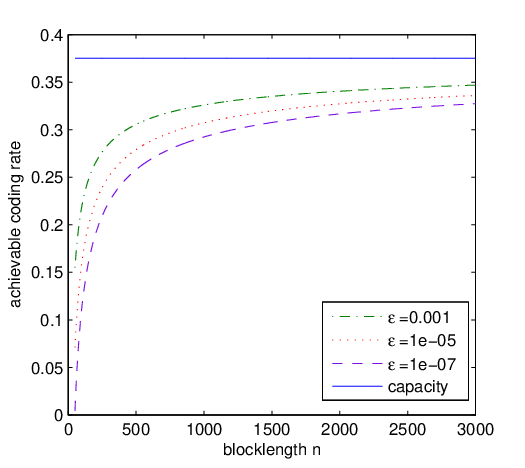
This confirms that $C$ is the operational capacity of the channel and any rate $R<C$ is achievable. The real beauty of Theorem 7 is, however, that we can use the asymptotic

as an approximation to the channel coding rate $\frac{\log N(n,\epsilon)}{n}$ and then anticipate the achievable rate on this channel in the finite block length regime. For illustraton we plotted this asymptotic for blocklengths ranging between $50$ and $3000$ and the example values $\lambda=0.2$, $\mu=0.8$ and $\epsilon=10^{-5}$ in Figure 3.

The Markov Chain $\Psi$ is aperiodic and irreducible. The state space of $\Psi_{i}$ can be chosen to be $\mathbb{X}=\boldsymbol{2}\times\mathbb{N}\cup\{(0,0)\}$. First we verify that Foster’s Criterion holds

By the results in [7] or Proposition A.5.7. in [8] the chain $\Psi$ is then geometrically ergodic.

By Theorem A.5.8. in [8] the asymptotic variance $\sigma^{2}$ is well defined, non-negative and finite, and

Finally, $f(\tilde{y},q)$ is a bounded, nonlattice (I still have to check that!), real-valued functional on the state space $\mathbb{X}$ and hence

where $p_{\Phi}(\xi)$ denotes the density of the standard Normal distribution $\Phi$, $\hat{f}$ is the solution to Poissons equation and $\eta$ is a constant [9]. The solution $\hat{f}$ can be chosen such that $\pi_{\Psi}(\hat{f})=0$ and the claim follows by averaging out $\psi_{0}$.

Using the representation of $\sigma^{2}$ in Equation 23 it remains to find explicit expressions for $\Var(f(\Psi_{0}))$ and the sum $\sum_{i=0}^{\infty}\Cov(f(\Psi_{0}),f(\Psi_{i}))$.

The term $\Var(f(\Psi_{0}))$ is easy to compute

Equation 35 holds true.

References

• [1] A. S. Bedekar and M. Azizoglu, “On the information-theoretic capacity of discrete-time queues,” IEEE Trans. Inform. Theory, vol. 44, pp. 446–461, 1998.
• [2] S. Meyn and R. L. Tweedie, Markov Chains and Stochastic Stability, 2nd ed. New York, NY, USA: Cambridge University Press, 2009.
• [3] R. M. Gray, Probability, Random Processes, and Ergodic Properties, 2nd ed. New York, NY, USA: Springer, 2009.
• [4] V. Anantharam and S. Verdu, “Bits through queues,” IEEE Trans. Inform. Theory, vol. 42, pp. 4–18, 1996.
• [5] H. Takagi, Queueing Analysis: A Foundation of Performance Evaluation. Amsterdam, The Netherlands: North Holland, 1993, vol. 3.
• [6] A. Feinstein, “A new basic theorem of information theory,” IRE Trans. Inform. Theory, vol. PGIT-4, pp. 2–22, 1954.
• [7] F. M. Spieksma and R. L. Tweedie, “Strengthening ergodicity to geometric ergodicity for markov chains,” Stochastic Models, vol. 10, pp. 45–75, 1994.
• [8] S. Meyn, Control Techniques for Complex Networks, 1st ed. New York, NY, USA: Cambridge University Press, 2007.
• [9] I. Kontoyiannis and S. Meyn, “Spectral theory and limit theorems for geometrically ergodic markov processes,” in the 2001 INFORMS Applied Probability Conference, 2001, pp. 304–362.
• [10] W. Whitt, “Asymptotic formulas for markov processes with applications to simulation,” Operations Research, vol. 40, pp. 279–291, 1992.
• [11] D. Y. Burman, “A functional central limit theorem for birth and death processes,” ORSA/TIMS Conference, 1980.
• [12] J. G. Kemeny and J. L. Snell, Finite Markov Chains. Princeton, N.J., USA: Van-Nostrand, 1960.
• [13] W. Grassmann, “The asymptotic variance of a time average in a birth-death process,” Annals of Operations Research, vol. 8, pp. 165–174, 1987.