Adiabatic continuity, wavefunction overlap and topological phase transitions

Within the non-interacting approximation, the many-body ground states of these two insulators can be written as

where $\ket{\textrm{G}_{I}}$ and $\ket{\textrm{G}_{II}}$ are the (many-body) ground states of the two insulators respectively. $\ket{0}$ represents the vacuum, i.e. the quantum state with no electrons. $c^{\dagger}_{\mathbf{k}}$ ($d^{\dagger}_{\mathbf{k}}$) is the creation operator which creates a particle in the Bloch state of the valence band in insulator $I$ (insulator $II$) at crystal momentum $\mathbf{k}$. $\prod_{\mathbf{k}}$ represents the product over all momenta in the Brillouin zone.

It is straightforward to verify that the overlap between the two ground states factorizes as

where $\phi(\mathbf{k})$ is the overlap between Bloch waves at crystal momentum $\mathbf{k}$

In the language of first quantization, this Bloch-wave overlap is

where

are the Bloch waves of the valence bands in insulators $I$ and $II$ respectively.

Define a new Bloch state

Here, $\ket{\psi^{I}(\mathbf{k})}$ and $\ket{\psi^{II}(\mathbf{k})}$ are the Bloch wavefunctions of the valence band for insulators $I$ and $II$ respectively [Eqs. (6) and (7)]. $\phi(\mathbf{k})^{*}=\braket{\psi^{II}(\mathbf{k})|\psi^{I}(\mathbf{k})}$ is the complex conjugate of the overlap between the two Bloch states as defined in Eq. (5). The control parameter $\alpha$ is a real number between $0$ and $1$. The denominator $\mathcal{N}$ is a normalization factor,

which enforces the normalization condition $\braket{\Psi(\mathbf{k},\alpha)|\Psi(\mathbf{k},\alpha)}=1$. It is easy to prove that as long as the overlap is nonzero $\phi\neq 0$, $\mathcal{N}$ is positive and thus the denominator will not introduce any singularity.

When $\alpha=0$, the Bloch state defined above coincides with $\ket{\psi^{I}(\mathbf{k})}$, i.e. the Bloch state for insulator $I$. At $\alpha=1$, the Bloch state becomes that of insulator $II$, up to an unimportant phase factor,

Therefore, by varying the parameter $0\leq\alpha\leq 1$, Eq. (8) defines a path between the two insulators.

As proved in Appendix B, if insulators $I$ and $II$ preserve certain symmetries (e.g., the time-reversal symmetry, lattice symmetries or some internal symmetries), the Bloch state $\ket{\Psi(\mathbf{k},\alpha)}$ will preserve the same symmetry. In other words, the path defined above preserves all necessary symmetries. This is very important for the study of symmetry-protected topological states.

Now, we explore one key problem for the study of adiabatic continuity: is it possible to use the path defined in Eq. (8) to deform insulator $I$ into insulator $II$ without closing the insulating gap?. The answer to this question is yes, as long as the wavefunction overlap remains finite for all momenta, $\phi(\mathbf{k})\neq 0$. To prove this conclusion, we construct the following hermitian operator, which will serve as the Hamiltonian for an insulator,

This Hamiltonian has one control parameter $0\leq\alpha\leq 1$. It has one flat band with energy $E=-1$ and the Bloch waves for this band is $\ket{\Psi(\mathbf{k},\alpha)}$. All other bands in the system have energy $E=0$. If we set the Fermi energy to be between $-1$ and $0$, this Hamiltonian defines a band insulator with one valence band. The band gap for this insulator is $1$.

When $\alpha=0$, the valence band has the same Bloch wavefunctions as insulator $I$, and for $\alpha=1$, the valence-band Bloch wavefunction coincides with that of insulator $II$. For $0<\alpha<1$, the Hamiltonian defines an insulator with a finite insulating gap, and the gap never closes. As a result, by varying the value of $\alpha$, the Hamiltonian shown in Eq. (12) defines an adiabatic path between the two insulators.

In the language of topological phase transitions, this observation implies that the two band insulators must belong to the same quantum phase (i.e. have the same topological indices), as long as the wavefunction overlap $\phi(\mathbf{k})$ remains finite for all $\mathbf{k}$. For two insulators with different topology (i.e. if some topological index takes different values in the two insulators), there must be at least one momentum point, at which the overlap vanishes.

In Eq. (8), we introduced a factor $\phi(\mathbf{k})^{*}$ in the definition of $\ket{\Psi(\mathbf{k},\alpha)}$. This factor is necessary in order to preserve the $U(1)$ phase symmetry, which is also known as the $U(1)$ gauge symmetry for band insulators [22]. In a band insulator, it is known that if we multiply a $U(1)$ phase to a Bloch wavefunction, the new wavefunction still describes the same Block state, i.e. $\ket{\psi^{I}(\mathbf{k})}$ and $e^{i\varphi}\ket{\psi^{I}(\mathbf{k})}$ describe the same Bloch state in insulator $I$, where $\varphi$ is an arbitrary $U(1)$ phase. Similarly, $\ket{\psi^{II}(\mathbf{k})}$ and $e^{i\varphi^{\prime}}\ket{\psi^{II}(\mathbf{k})}$ correspond to the same Bloch state in insulator $II$. In other words, when we write down the Bloch states $\ket{\psi^{I}(\mathbf{k})}$ and $\ket{\psi^{II}(\mathbf{k})}$ for the insulators, there is a freedom to choose an arbitrary phase factor for each of these states. In order to ensure that physical observables [e.g. the Hamiltonian $H(\alpha)$] does not depend on this arbitrary phase choice, the factor $\phi(\mathbf{k})^{*}$ is necessary. It is straightforward to verify that with the help of this factor, the Hamiltonian $H(\alpha)$ defined in Eq. (12) is independent of the phase choice, i.e. it is invariant under the transformation

In addition, as shown in Appendix B, this factor $\phi(\mathbf{k})^{*}$ also helps to ensure that the adiabatic path preserves the same symmetries as insulators $I$ and $II$.

For an insulator with $N$ valence bands, in the non-interacting limit, the ground state wavefunction is

Here, we follow the same convention as utilized in Eqs. (1) and (2), except that the creation operators $c^{\dagger}_{n,\mathbf{k}}$ now have one extra subindex $n$, which labels the valence bands ($n=1,2,\ldots,N$), and $\prod_{n=1}^{N}$ represents the product for all occupied bands.

Consider another insulator with the same number of valence band, whose ground state wavefunction is

where $d^{\dagger}_{n,\mathbf{k}}$ is the creation operator for the Bloch waves in this insulator. The quantum overlap between the two ground states of these two insulators factorizes (similar to the case with one valence band)

where the Bloch-wave overlap at each momentum point is

In the first-quantization language, $\phi(\mathbf{k})$ is the determinant of the overlap matrix $\mathcal{F}(\mathbf{k})$

where $\mathcal{F}(\mathbf{k})$ is a $N\times N$ matrix with matrix elements

where

are the Bloch wavefunctions of the valence bands for insulators $I$ and $II$ respectively, and the subindices $n$ and $m$ are band indices for valence bands in these two insulators.

We emphasize that the overlap matrix $\mathcal{F}(\mathbf{k})$ is a function of the crystal momentum $\mathbf{k}$. However, to simplify the formulas, in this article we will use $\mathcal{F}$ to represent the matrix without showing explicitly that this matrix is a function of $\mathbf{k}$.

In this section, we will assume that the overlap between the two insulators, i.e. $\phi(\mathbf{k})$ defined in Eq. (18), is finite for all momentum points, and then define an adiabatic path between the two insulators.

According to Eq. (19), $\phi(\mathbf{k})\neq 0$ implies that the overlap matrix $\mathcal{F}$ [Eq. (20)] has a nonzero determinant. As shown in Appendix A.2, because $\mathcal{F}\mathcal{F}^{\dagger}$ is a hermitian matrix, we can find a unitary matrix $\mathcal{U}$, which diagonalizes $\mathcal{F}\mathcal{F}^{\dagger}$, i.e. $\mathcal{U}\mathcal{F}\mathcal{F}^{\dagger}\mathcal{U}^{\dagger}$ is a diagonal matrix. Utilizing the matrices $\mathcal{F}$ and $\mathcal{U}$, we can define $N$ quantum states

where $*$ represents complex conjugate; $0\leq\alpha\leq 1$ is a control parameter and the subindex $l=1,2,\ldots,N$. In this article, we adopt the Einstein summation convention. Unless claimed otherwise, repeated band indices will be summed over, and this sum only goes over all valence bands with band indices between $1$ and $N$, while conduction bands (with band indices larger than $N$) will not be included in the sum. The denominator $\mathcal{N}_{l}$ is the normalization factor, which ensures that the quantum state is properly normalized, $\braket{\Psi_{l}|\Psi_{l}}=1$, and the value of this normalization function is shown in Eq (74). In Appendix A.4, we proved that this normalization factor $\mathcal{N}_{l}$ never reaches zero, as long as the overlap is nonzero $\phi(\mathbf{k})\neq 0$, which ensures that Eq. (23) is singularity free.

We will prove in the next section that as long as the overlap $\phi(\mathbf{k})$ remains finite, the states defined in Eq. (23) are orthonormal

As a result, we can design an insulator with $N$ valence bands and utilize these orthonormal states as the Bloch states of the valence bands, and this insulator will serve as an adiabatic path between insulators $I$ and $II$. Here, we define the Hamiltonian of this insulator

Because $\ket{\Psi_{l}(\mathbf{k},\alpha)}$ are orthonormal for $l=1,2,\ldots,N$, it is straightforward to verify that $\ket{\Psi_{l}(\mathbf{k},\alpha)}$ are eigenstates of the Hamiltonian with eigenenergy $E=-1$, and all other single-particle states orthogonal to $\ket{\Psi_{l}(\mathbf{k},\alpha)}$ have eigenenergy $E=0$, i.e., this Hamiltonian has $N$ (flat) energy bands with energy $E=-1$ and all other energy bands have energy $E=0$. If the Fermi energy is between $-1$ and $0$, this Hamiltonian defines a band insulator with band gap $\Delta=1$, and $\ket{\Psi_{l}(\mathbf{k},\alpha)}$ are the Bloch waves of the valence bands. As will be shown in the next section, for $\alpha=0$ ($\alpha=1$), the ground state wavefunction of this insulator coincides with that of insulator $I$ (insulator $II$). And thus $H(\alpha)$ defines an adiabatic path between the two insulators.

In this section, we prove the conclusions presented in Sec. II.2.2. We will first prove that the quantum states defined in Eq. (23) are indeed orthonormal, i.e., $\braket{\Psi_{l}(\mathbf{k},\alpha)|\Psi_{l^{\prime}}(\mathbf{k},\alpha)}=\delta_{l,l^{\prime}}$ Then, we will show that the Hamiltonian defined in Eq. (25) is the Hamiltonian for an insulator with $N$ valence bands, and we will further prove that for $\alpha=0$ ($\alpha=1$), the ground state recovers that of the insulator $I$ ($II$).

It turns out that it is easier to present the proof using second quantization, so here we will reformulate the same Bloch states and the Hamiltonian utilizing creation/annihilation operators defined in Eqs. (15) and (16), i.e. the creation operator $c^{\dagger}_{n,\mathbf{k}}$ ($d^{\dagger}_{m,\mathbf{k}}$) adds one electron to the $n$th ($m$th) valence band of insulator $I$ ($II$) at crystal momentum $\mathbf{k}$. Since electrons are fermions, the creation/annihilation operators satisfy the canonical anti-commutation relation

where $\delta$ is the Kronecker delta. For the anti-commutators between $c$s and $d$s, it is straightforward to prove that

(See Appendix A.1 for details).

Utilizing these creation and annihilation operators, as well as the matrices $\mathcal{F}$ and $\mathcal{U}$ defined in Sec II.2.2, we can define creation operators

Here, repeated indices are summed over, same as in Eq. (23). It is straightforward to verify that this creation operator creates the Bloch state $\ket{\Psi_{l}(\mathbf{k},\alpha)}$ defined in Eq. (23), i.e. $\ket{\Psi_{l}(\mathbf{k},\alpha)}=a^{\dagger}_{l,\mathbf{k}}\ket{0}$. In Appendix A.3, we proved that as long as the overlap $\phi(\mathbf{k})$ is nonzero, these $a^{\dagger}_{l,\mathbf{k}}$ operators, and the corresponding annihilation operators, satisfies canonical anti-commutation relations

The anti-commutation relation implies that the quantum states defined in Eq. (23) are orthonormal, because

Now we examine the Hamiltonian defined in Eq.(25) and rewrite it in the second-quantization language

Along with the anti-commutation relation [Eq. (31)], it is easy to verify that this Hamiltonian describes a band insulator with $N$ valence bands. $a^{\dagger}_{l,\mathbf{k}}$ are the creation operators for the Bloch states in the valence bands ($l=1,2,\ldots,N$). All the valence bands in this insulator have energy $-1$, while the conduction bands have energy $0$. Here, we set the Fermi energy into the band gap, i.e., between $-1$ and $0$. For any values of $0\leq\alpha\leq 1$, the insulating gap never closes and the value remains $1$.

For $\alpha=0$, we know from Eq. (30) that

Because $\mathcal{U}$ is a unitary matrix (i.e. $\mathcal{U}^{*}_{l,n}\mathcal{U}_{l,n^{\prime}}=\delta_{n,n^{\prime}}$), the Hamiltonian at $\alpha=0$ is

Therefore, the ground state is identical to that of insulator $I$, i.e., all Bloch states created by $c^{\dagger}_{n,\mathbf{k}}$ for $n=1,2,\ldots,N$ are occupied.

For $\alpha=1$, Eq. (30) implies that

Thus the Hamiltonian becomes

As proved in Appendix A.2,

and thus this Hamiltonian can be simplified

The ground state for this Hamiltonian coinides with that of the insulator $II$, i.e., all Bloch states created by $d^{\dagger}_{m,\mathbf{k}}$ for $m=1,2,\ldots,N$ are occupied.

Consider two insulators with different numbers of valence bands. It is easy to realize that these two insulators are not adiabatically connected, because it is impossible to change the number of valence bands in a band insulator without going through a gapless (metallic) state.

At the same time, we know that the overlap function also vanishes. Utilizing the overlap function defined in Eq. (18), we know that

where $N$ and $N^{\prime}$ are the number of valence bands for the two insulators respectively. It is transparent that $\phi(\mathbf{k})=0$, if $N\neq N^{\prime}$.

In summary, for two insulators with different numbers of valence bands, the two insulators are not adiabatically connected, and the wavefunction overlap is zero.

First, we consider insulators with different topological structures and show that the wavefunction overlap must vanish at some moment point. We start by considering the model of Haldane [2]. As pointed out by Haldane, for a honeycomb lattice, the Dirac band-touching point can be gapped by two different methods: (1) introducing a magnetic flux pattern, which breaks the time-reversal symmetry or (2) introducing a staggered potential, which breaks the degeneracy between the two sublattices. At half-filling, these two approaches result in two different insulators with different topology, a topologically-nontrivial Chern insulator and a topologically-trivial conventional insulator.

Utilizing these two topologically different insulators, we can compute the overlap between Bloch states in their valence bands, i.e., $\phi(\mathbf{k})$ defined above. As shown in Fig. 1, this overlap vanishes at the $K$ point, in agreement with our conclusions above.

For Chern insulators with different Chern numbers, zero wavefunction overlap has been observed and proved in earlier studies using other approaches [23, 24]. Our theorem indicates that the same conclusions will remain for any types of topological indices, including symmetry-protected topological states. To demonstrate this conclusion, we have also computed the wavefunction overlap in other models with one or more valence bands (not shown), e.g. the Kane-Mele model [25] and the Bernevig-Hughes-Zhang model [26]. For insulating states with different topology, we always find some momentum point, at which the wavefunction overlap $\phi(\mathbf{k})$ reaches zero.

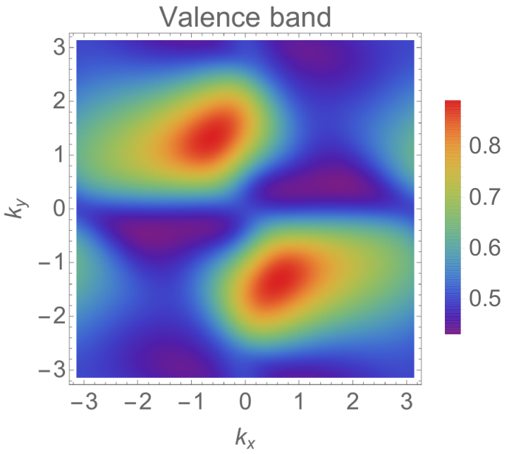
Here, we consider two topologically equivalent insulators with different lattice structures. In this example, we compare the quantum spin Hall insulators in the Kane-Mele model [25] and the Bernevig-Hughes-Zhang model [26].

These two models assum very different lattice structures (honeycomb and square) and thus the Brillouin zones of these two models have very different geometry. As shown in Appendix (Sec. C), we can use a continuous one-to-one correspondence to map the Brillouin zone of the Kane-Mele model to that of the Bernevig-Hughes-Zhang model. (There exist infinite many such mappings, and here we just adopt one of them to demonstrate the physics). As shown in Fig. 2, despite differences in lattice structures etc., the quantum-spin-Hall insulators described by these two different models show finite wavefunction overlap, which implies immediately that they are topologically equivalent.

Consider a finite-size two-dimensional many-body systems with size $L_{x}\times L_{y}$. We enforce twisted boundary conditions for many-body wavefunctions

where $\psi$ is a many-body wavefunction, while $x_{i}$ and $y_{i}$ are the $x$ and $y$ cooridnates of the $i$th particle. $\varphi_{x}$ and $\varphi_{y}$ are two phase factors. For $\varphi_{x}=\varphi_{y}=0$ ($\varphi_{x}=\varphi_{y}=\pi$), it recovers the periodic (anti-periodic) boundary conditions. For other values of $\varphi_{x}$ and $\varphi_{y}$, it is known as the twisted boundary conditions.

We can find the ground state of a quantum system under twisted boundary conditions $\ket{\psi(\varphi_{x},\varphi_{y})}$. In general, the ground state wavefunction depends on the values of $\varphi_{x}$ and $\varphi_{y}$. For a gapped system, we can define the following integral

As pointed out in Ref. 28, this integral is a topological invariant, i.e. the first Chern number, regardless of the size of the system. In the thermodynamic limit, this topological index coincides with the Hall conductivity [28]. Because the definition utilizes many-body wavefunctions (without using single-particle Bloch waves), it is applicable for both interacting and non-interacting systems. In the non-interacting limit, it recovers the Chern number computed using single-particle Bloch waves [29].

It is also worthwhile to mention that it is straightforward to generalize this definition to fractional quantum Hall systems and fractional Chern insulators. Once topological degeneracy is taken into account, the integral shown above produces fractional values, i.e. the fractional Hall conductivity [30].

Consider a 2D finite-size system with Hamiltonian $H_{1}$ and another 2D system with the same size but a different Hamiltonian $H_{2}$. Here, we allow the Hamiltonians to contain interactions, and we assume that the ground states are gapped for both Hamiltonians (for any twisted boundary conditions). We can find the many-body ground states for the two Hamiltonians under twisted boundary condition $\ket{\psi_{1}(\varphi_{x},\varphi_{y})}$ and $\ket{\psi_{2}(\varphi_{x},\varphi_{y})}$ respectively. Using Eq. (50), one can compute the Chern number for the ground states of both Hamiltonians.

Here, we ask the following question: if the ground states of the two Hamiltonians have different Chern numbers, what is the wavefunction overlap between the two insulators, $\braket{\psi_{1}(\varphi_{x},\varphi_{y})|\psi_{2}(\varphi_{x},\varphi_{y})}$. Because we have set the system-size to finite, the wavefunction overlap does not suffer from the orthogonality catastrophe, and thus we can directly apply the theorem proved above.

Because the two ground states have different Chern numbers, it is impossible to adiabatically deform one state into the other without closing the excitation gap (between the ground state and the first excited state). This implies that no matter how we try to deform $H_{1}$ into $H_{2}$, adiabatically, the excitation gap must close for at least one set of $\varphi_{x}$ and $\varphi_{y}$. Utilizing the theorem proved above, this implies that we can find at least one set of $\varphi_{x}$ and $\varphi_{y}$, the wavefunction overlap vanishes $\braket{\psi_{1}(\varphi_{x},\varphi_{y})|\psi_{2}(\varphi_{x},\varphi_{y})}=0$. Otherwise, an adiabatic path will exist, which is in contradiction to the assumption that the two states have different Chern numbers.

Now we consider the opposite situation, where $\braket{\psi_{1}(\varphi_{x},\varphi_{y})|\psi_{2}(\varphi_{x},\varphi_{y})}\neq 0$ for all possible values of $\varphi_{x}$ and $\varphi_{y}$. Utilizing the theorem shown above, for any twisted boundary condition, we can construct an adiabatic path between these two quantum states without closing the gap. As a result, the two states must have the same Chern number.

Now we study a topological phase transitions in a 2D interacting system. Consider a Hamiltonian $H(\alpha)$, where $\alpha$ is a control parameter. We assume that by tuning the control parameter $\alpha$, the system undergoes a topological phase transition, where the Chern number changes its value, i.e., the Hamiltonian has a gapped ground state for both $\alpha>\alpha_{C}$ and $\alpha<\alpha_{C}$, but the ground states have different Chern numbers for $\alpha>\alpha_{C}$ and $\alpha<\alpha_{C}$. Here again, we consider a finite-size system, although one can take the thermodynamic limit later via finite size scaling. As shown above and pointed out in Ref. 31, even for finite size systems, the Chern number and the topological phase transition is well-defined.

The ground-state wavefunction of this Hamiltonian, $\ket{\psi_{\alpha}(\varphi_{x},\varphi_{y})}$ depends on the value of the control parameter $\alpha$, as well as the phases of the twisted boundary conditions $\varphi_{x}$ and $\varphi_{y}$. We can compute the wavefunction overlap for the ground states at different values of $\alpha$,

The conclusions that we proved above indicate immediately that if this overlap never vanishes for any $\varphi_{x}$ and $\varphi_{y}$, $H(\alpha_{1})$ and $H(\alpha_{2})$ describe states in the same quantum phase, i.e. $\alpha_{1}>\alpha_{C}$ and $\alpha_{2}>\alpha_{C}$, or $\alpha_{1}<\alpha_{C}$ and $\alpha_{2}<\alpha_{C}$.

Similarly. if we compute the overlap for two wavefunctions from two different topological phases, (e.g., $\alpha_{1}>\alpha_{C}$ and $\alpha_{2}<\alpha_{C}$), then this overlap must vanish for some values of $\varphi_{x}$ and $\varphi_{y}$. A special case of this type has been shown in Ref. 31, where $\alpha_{1}$ and $\alpha_{2}$ are very close to the transition point, i.e. $\alpha_{1}=\alpha_{C}+\epsilon$ and $\alpha_{2}=\alpha_{C}-\epsilon$ where $\epsilon$ is a very small positive number. There, the vanishing wavefunction overlap results in a singularity (i.e. a Dirac $\delta$-function) in the fidelity matrix [32, 33, 34], which can be used to pin-point the topological phase transition in a finite-size interacting system. The results shown above generalize the same conclusion for any values of $\alpha_{1}>\alpha_{C}$ and $\alpha_{2}<\alpha_{C}$, close or far away from the topological transition point.

References

- [1] S. Sachdev, Quantum Phase Transitions (Cambridge University Press, Cambridge, UK, 1999).
- [2] F. D. M. Haldane, Phys. Rev. Lett. 61, 2015 (1988).
- [3] M. Z. Hasan and C. L. Kane, Rev. Mod. Phys. 82, 3045 (2010).
- [4] X.-L. Qi and S.-C. Zhang, Rev. Mod. Phys. 83, 1057 (2011).
- [5] B. A. Bernevig and T. L. Hughes, Topological Insulators and Topological Superconductors (Princeton University Press, 2013).
- [6] A. Kitaev, AIP Conf. Proc. 1134, 22 (2009).
- [7] A. P. Schnyder, S. Ryu, A. Furusaki, and A. W. W. Ludwig, Phys. Rev. B 78, 195125 (2008).
- [8] J. E. Moore, Y. Ran, and X.-G. Wen, Phys. Rev. Lett. 101, 186805 (2008).
- [9] L. Fu, Phys. Rev. Lett. 106, 106802 (2011).
- [10] P. W. Anderson, Phys. Rev. Lett. 18, 1049 (1967).
- [11] K. von Klitzing, G. Dorda, and M. Pepper, Phys. Rev. Lett. 45, 494 (1980).
- [12] D. C. Tsui, H. L. Stormer, and A. C. Gossard, Phys. Rev. Lett. 48, 1559 (1982).
- [13] A. Kol and N. Read, Phys. Rev. B 48, 8890 (1993).
- [14] A. S. Sørensen, E. Demler, and M. D. Lukin, Phys. Rev. Lett. 94, 086803 (2005).
- [15] G. Möller and N. R. Cooper, Phys. Rev. Lett. 103, 105303 (2009).
- [16] E. Tang, J.-W. Mei, and X.-G. Wen, Phys. Rev. Lett. 106, 236802 (2011).
- [17] K. Sun, Z. Gu, H. Katsura, and S. Das Sarma, Phys. Rev. Lett. 106, 236803 (2011).
- [18] T. Neupert, L. Santos, C. Chamon, and C. Mudry, Phys. Rev. Lett. 106, 236804 (2011).
- [19] D. N. Sheng, Z.-C. Gu, K. Sun, and L. Sheng, Nat. Commun. 2, 389 (2011).
- [20] N. Regnault and B. A. Bernevig, Phys. Rev. X 1, 021014 (2011).
- [21] S. A. Parameswaran, R. Roy, and S. L. Sondhi, Comptes Rendus Physique 14, 816 (2013).
- [22] E. I. Blount, in Solid State Physics, Vol. 13, edited by F. Seitz and D. Turnbull (Academic, New York, 1962).
- [23] B.-J. Yang, M. S. Bahramy, and N. Nagaosa, Nat. Commun. 4, 1524 (2013).
- [24] Z. Huang and A. V. Balatsky, arXiv:1604.04698 (2016).
- [25] C. L. Kane and E. J. Mele, Phys. Rev. Lett. 95, 146802 (2005).
- [26] B. A. Bernevig, T. L. Hughes, and S.-C. Zhang, Science 314, 1757 (2006).
- [27] Y.-Z. You, Z. Bi, A. Rasmussen, K. Slagle, and C. Xu, Phys. Rev. Lett. 112, 247202 (2014).
- [28] Q. Niu, D. J. Thouless, and Y.-S. Wu, Phys. Rev. B 31, 3372 (1985).
- [29] D. J. Thouless, M. Kohmoto, M. P. Nightingale, and M. den Nijs, Phys. Rev. Lett. 49, 405 (1982).
- [30] D. N. Sheng, X. Wan, E. H. Rezayi, K. Yang, R. N. Bhatt, and F. D. M. Haldane, Phys. Rev. Lett. 90, 256802 (2003).
- [31] C. N. Varney, K. Sun, M. Rigol, and V. Galitski, Phys. Rev. B 84, 241105 (2011).
- [32] P. Zanardi and N. Paunković, Phys. Rev. E 74, 031123 (2006).
- [33] L. Campos Venuti and P. Zanardi, Phys. Rev. Lett. 99, 095701 (2007).
- [34] M. Rigol, B. S. Shastry, and S. Haas, Phys. Rev. B 80, 094529 (2009).
- [35] Y.-Y. He, H.-Q. Wu, Y.-Z. You, C. Xu, Z. Y. Meng, and Z.-Y. Lu, Phys. Rev. B 93, 115150 (2016).