跳到论文正文
W Papers独立论文阅读器 arXiv:1605.07583 论文正文 计算阅读时间 · 0%
引用这篇论文根据当前论文元数据生成,正式投稿前建议核对。


License: arXiv.org perpetual non-exclusive license
arXiv:1605.07583v5 [cs.LG] 03 Nov 2017

Recursive Sampling for the Nyström Method

Cameron Musco Affiliation: MIT Email: cnmusco@mit.edu    Christopher Musco Affiliation: MIT Email: cpmusco@mit.edu
Abstract

We give the first algorithm for kernel Nyström approximation that runs in linear time in the number of training points and is provably accurate for all kernel matrices, without dependence on regularity or incoherence conditions. The algorithm projects the kernel onto a set of ss landmark points sampled by their ridge leverage scores, requiring just O⁡(n​s)O(ns) kernel evaluations and O⁡(n​s2)O(ns^{2}) additional runtime. While leverage score sampling has long been known to give strong theoretical guarantees for Nyström approximation, by employing a fast recursive sampling scheme, our algorithm is the first to make the approach scalable. Empirically we show that it finds more accurate, lower rank kernel approximations in less time than popular techniques such as uniformly sampled Nyström approximation and the random Fourier features method.

1 Introduction

The kernel method is a powerful tool for applying linear learning algorithms (SVMs, linear regression, etc.) to nonlinear problems. The key idea is to map data to a higher dimensional kernel feature space, where linear relationships correspond to nonlinear relationships in the original data.

Typically this mapping is implicit. A kernel function is used to compute inner products in the high-dimensional kernel space, without ever actually mapping original data points to the space. Given nn data points 𝐱1,…,𝐱n\mathbf{x}_{1},\ldots,\mathbf{x}_{n}, the n×nn\times n kernel matrix 𝐊\mathbf{K} is formed where 𝐊i,j\mathbf{K}_{i,j} contains the high-dimensional inner product between 𝐱i\mathbf{x}_{i} and 𝐱j\mathbf{x}_{j}, as computed by the kernel function. All computations required by a linear learning method are performed using the inner product information in 𝐊\mathbf{K}.

Unfortunately, the transition from linear to nonlinear comes at a high cost. Just generating the entries of 𝐊\mathbf{K} requires Θ⁡(n2)\Theta(n^{2}) time, which is prohibitive for large datasets.

1.1 Kernel approximation

A large body of work seeks to accelerate kernel methods by finding a compressed, often low-rank, approximation 𝐊~\mathbf{\tilde{K}} to the true kernel matrix 𝐊\mathbf{K}. Techniques include random sampling and embedding [AMS01, BBV06, ANW14], random Fourier feature methods for shift invariant kernels [RR07, RR09, LSS13], and incomplete Cholesky factorization [FS02, BJ02].

One of the most popular techniques is the Nyström method, which constructs 𝐊~\mathbf{\tilde{K}} using a subset of “landmark” data points [WS01]. Once ss data points are selected, 𝐊~\mathbf{\tilde{K}} (in factored form) takes just O⁡(n​s)O(ns) kernel evaluations and O⁡(s3)O(s^{3}) additional time to compute, requires O⁡(n​s)O(ns) space to store, and can be manipulated quickly in downstream applications. E.g., inverting 𝐊~\mathbf{\tilde{K}} takes O⁡(n​s2)O(ns^{2}) time.

The Nyström method performs well in practice [YLM+12, GM13, TRVR16], is widely implemented [HFH+09, PVG+11, IBM14], and is used in many applications under different names such as “landmark isomap” [DST03] and “landmark MDS” [Pla05]. In the classic variant, landmark points are selected uniformly at random. However, significant research seeks to improve performance via data-dependent sampling that selects landmarks which more closely approximate the full kernel matrix than uniformly sampled ones [SS00, DM05, ZTK08, BW09, KMT12, WZ13, GM13, LJS16].

Theoretical work has converged on leverage score based approaches, as they give the strongest provable guarantees for both kernel approximation [DMM08, GM13] and statistical performance in downstream applications [AM15, RCR15, Wan16]. Leverage scores capture how important an individual data point is in composing the span of the kernel matrix.

Unfortunately, these scores are prohibitively expensive to compute. All known approximation schemes require Ω⁡(n2)\Omega(n^{2}) time or assume strong conditions on 𝐊\mathbf{K} – e.g. good conditioning or data “incoherence” [DMIMW12, GM13, AM15, CLV16]. Hence, leverage score-based approaches remain largely in the domain of theory, with limited practical impact [KMT12, LBKL15, YPW15].

1.2 Our contributions

In this work, we close the gap between strong approximation bounds and efficiency: we present a new Nyström algorithm based on recursive leverage score sampling which achieves the “best of both worlds”: it produces kernel approximations provably matching the accuracy of leverage score methods while only requiring O⁡(n​s)O(ns) kernel evaluations and O⁡(n​s2)O(ns^{2}) runtime for ss landmark points.

Theoretically, this runtime is surprising. In the typical case when s≪ns\ll n, the algorithm evaluates just a small subset of 𝐊\mathbf{K}, ignoring most of the kernel space inner products. Yet its performance guarantees hold for general kernels, requiring no assumptions on coherence or regularity.

Empirically, the runtime’s linear dependence on nn means that our method is the first leverage score algorithm that can compete with the most commonly implemented techniques, including the classic uniform sampling Nyström method and random Fourier features sampling [RR07]. Since our algorithm obtains higher quality samples, we show experimentally that it outperforms these methods on benchmark datasets – it can obtain as accurate a kernel approximation in significantly less time. As a bonus, our approximations have lower rank, so they can be stored in less space and processed more quickly in downstream learning tasks.

1.3 Paper outline

Our recursive sampling algorithm is built on top of a Nyström scheme of Alaoui and Mahoney that samples landmark points based on their ridge leverage scores [AM15]. After reviewing preliminaries in Section 2, in Section 3 we analyze this scheme, which we refer to as RLS-Nyström. To simplify prior work, which studies the statistical performance of RLS-Nyström for specific kernel learning tasks [AM15, RCR15, Wan16], we prove a strong, application independent approximation guarantee: for any λ\lambda, if 𝐊~\mathbf{\tilde{K}} is constructed with s=Θ⁡(deffλ​log⁡deffλ)s=\Theta(d_{\text{eff}}^{\lambda}\log d_{\text{eff}}^{\lambda}) samples11 1 O⁡(deffλ​log⁡deffλ)O(d_{\text{eff}}^{\lambda}\log d_{\text{eff}}^{\lambda}) samples is within a log factor of the best possible for any low-rank approximation with error λ\lambda., where deffλ=tr⁡(𝐊​(𝐊+λ​𝐈)−1)d_{\text{eff}}^{\lambda}=\tr(\mathbf{K}(\mathbf{K}+\lambda\mathbf{I})^{-1}) is the so-called “λ\lambda-effective dimensionality” of 𝐊\mathbf{K}, then with high probability, ‖𝐊−𝐊~‖2≤λ.\|\mathbf{K}-\mathbf{\tilde{K}}\|_{2}\leq\lambda.

In Appendix C, we show that this guarantee implies prior results on the statistical performance of RLS-Nyström for kernel ridge regression and canonical correlation analysis. We also use it to prove new results on the performance of RLS-Nyström for kernel rank-kk PCA and kk-means clustering – in both cases just O⁡(k​log⁡k)O(k\log k) samples are required to give a solution with good accuracy.

After affirming the favorable theoretical properties of RLS-Nyström, in Section 4 we show that its runtime can be significantly improved using a recursive sampling approach. Intuitively our algorithm is simple. We show how to approximate the kernel ridge leverage scores using a uniform sample of 12\frac{1}{2} of our input points. While the subsampled kernel matrix still has a prohibitive n2/4n^{2}/4 entries, we can recursively approximate it, using our same sampling algorithm. If our final Nyström approximation will use ss landmarks, the recursive approximation only needs rank O⁡(s)O(s), which lets us estimate the ridge leverage scores of the original kernel matrix in just O⁡(n​s2)O(ns^{2}) time. Since nn is cut in half at each level of recursion, our total runtime is O⁡(n​s2+n​s22+n​s24+…)=O⁡(n​s2)O\left(ns^{2}+\frac{ns^{2}}{2}+\frac{ns^{2}}{4}+...\right)=O(ns^{2}), significantly improving upon the method of [AM15], which takes Θ⁡(n3)\Theta(n^{3}) time in the worst case.

Our approach builds on recent work on iterative sampling methods for approximate linear algebra [CLM+15, CMM17]. While the analysis in the kernel setting is technical, our final algorithm is simple and easy to implement. We present and test a parameter-free variation of Recursive RLS-Nyström in Section 5, confirming superior performance compared to existing methods.

2 Preliminaries

Consider an input space 𝒳\mathcal{X} and a positive semidefinite kernel function K:𝒳×𝒳→ℝK:\mathcal{X}\times\mathcal{X}\rightarrow\mathbb{R}. Let ℱ\mathcal{F} be an associated reproducing kernel Hilbert space and ϕ:𝒳→ℱ\phi:\mathcal{X}\rightarrow\mathcal{F} be a (typically nonlinear) feature map such that for any 𝐱,𝐲∈𝒳\mathbf{x},\mathbf{y}\in\mathcal{X}, K⁡(𝐱,𝐲)=⟨ϕ⁡(𝐱),ϕ⁡(𝐲)⟩ℱK(\mathbf{x},\mathbf{y})=\langle\phi(\mathbf{x}),\phi(\mathbf{y})\rangle_{\mathcal{F}}. Given a set of nn input points 𝐱1,…,𝐱n∈𝒳\mathbf{x}_{1},\ldots,\mathbf{x}_{n}\in\mathcal{X}, define the kernel matrix 𝐊∈ℝn×n\mathbf{K}\in\mathbb{R}^{n\times n} by 𝐊i,j=K⁡(𝐱i,𝐱j).\mathbf{K}_{i,j}=K(\mathbf{x}_{i},\mathbf{x}_{j}).

It will often be natural to consider the kernelized data matrix that generates 𝐊\mathbf{K}. Informally, let 𝚽∈ℝn×d′\mathbf{\Phi}\in\mathbb{R}^{n\times d^{\prime}} be the matrix containing ϕ⁡(𝐱1),…,ϕ⁡(𝐱n)\phi(\mathbf{x}_{1}),...,\phi(\mathbf{x}_{n}) as its rows (note that d′d^{\prime} may be infinite). 𝐊=𝚽​𝚽T\mathbf{K}=\mathbf{\Phi}\mathbf{\Phi}^{T}. While we use 𝚽\mathbf{\Phi} for intuition, in our formal proofs we replace it with any matrix 𝐁∈ℝn×n\mathbf{B}\in\mathbb{R}^{n\times n} satisfying 𝐁𝐁T=𝐊\mathbf{B}\mathbf{B}^{T}=\mathbf{K} (e.g. a Cholesky factor).

We repeatedly use the singular value decomposition, which allows us to write any rank rr matrix 𝐌∈ℝn×d\mathbf{M}\in\mathbb{R}^{n\times d} as 𝐌=𝐔​𝚺​𝐕𝐓\mathbf{M}=\mathbf{U}\mathbf{\Sigma}\mathbf{V^{T}}, where 𝐔∈ℝn×r\mathbf{U}\in\mathbb{R}^{n\times r} and 𝐕∈ℝd×r\mathbf{V}\in\mathbb{R}^{d\times r} have orthogonal columns (the left and right singular vectors of 𝐌\mathbf{M}), and 𝚺∈ℝr×r\mathbf{\Sigma}\in\mathbb{R}^{r\times r} is a positive diagonal matrix containing the singular values: σ1​(𝐌)≥σ2​(𝐌)≥…≥σr​(𝐌)>0\sigma_{1}(\mathbf{M})\geq\sigma_{2}(\mathbf{M})\geq\ldots\geq\sigma_{r}(\mathbf{M})>0. 𝐌\mathbf{M}’s pseudoinverse is given by 𝐌+=𝐕​𝚺−1​𝐔T\mathbf{M}^{+}=\mathbf{V}\mathbf{\Sigma}^{-1}\mathbf{U}^{T}.

2.1 Nyström approximation

The Nyström method selects a subset of “landmark” points and uses them to construct a low-rank approximation to 𝐊\mathbf{K}. Given a matrix 𝐒∈ℝn×s\mathbf{S}\in\mathbb{R}^{n\times s} that has a single entry in each column equal to 11 so that 𝐊𝐒\mathbf{K}\mathbf{S} is a subset of ss columns from 𝐊\mathbf{K}, the associated Nyström approximation is:

𝐊~=𝐊𝐒​(𝐒T​𝐊𝐒)+​𝐒T​𝐊.\displaystyle\mathbf{\tilde{K}}=\mathbf{KS}(\mathbf{S}^{T}\mathbf{KS})^{+}\mathbf{S}^{T}\mathbf{K}. (1)

𝐊~\mathbf{\tilde{K}} can be stored in O⁡(n​s)O(ns) space by separately storing 𝐊𝐒∈ℝn×s\mathbf{KS}\in\mathbb{R}^{n\times s} and (𝐒T​𝐊𝐒)+∈ℝs×s(\mathbf{S}^{T}\mathbf{KS})^{+}\in\mathbb{R}^{s\times s}. Furthermore, the factors can be computed using just O⁡(n​s)O(ns) evaluations of the kernel inner product to form 𝐊𝐒\mathbf{K}\mathbf{S} and O⁡(s3)O(s^{3}) time to compute (𝐒T​𝐊𝐒)+(\mathbf{S}^{T}\mathbf{KS})^{+}. Typically s≪ns\ll n so these costs are significantly lower than the cost to form and store the full kernel matrix 𝐊\mathbf{K}.

We view Nyström approximation as a low-rank approximation to the dataset in feature space. Recalling that 𝐊=𝚽​𝚽T\mathbf{K}=\mathbf{\Phi}\mathbf{\Phi}^{T}, 𝐒\mathbf{S} selects ss kernelized data points 𝐒T​𝚽\mathbf{S}^{T}\mathbf{\Phi} and we approximate 𝚽\mathbf{\Phi} using its projection onto these points. Informally, let 𝐏𝐒∈ℝd′×d′\mathbf{P}_{\mathbf{S}}\in\mathbb{R}^{d^{\prime}\times d^{\prime}} be the orthogonal projection onto the row span of 𝐒T​𝚽\mathbf{S}^{T}\mathbf{\Phi}. We approximate 𝚽\mathbf{\Phi} by 𝚽~=def𝚽​𝐏𝐒\mathbf{\tilde{\Phi}}\mathbin{\stackrel{{\scriptstyle\rm def}}{{=}}}\mathbf{\Phi}\mathbf{P}_{\mathbf{S}}. We can write 𝐏𝐒=𝚽T​𝐒​(𝐒T​𝚽​𝚽T​𝐒)+​𝐒T​𝚽\mathbf{P}_{\mathbf{S}}=\mathbf{\Phi}^{T}\mathbf{S}(\mathbf{S}^{T}\mathbf{\Phi}\mathbf{\Phi}^{T}\mathbf{S})^{+}\mathbf{S}^{T}\mathbf{\Phi}. Since it is an orthogonal projection, 𝐏𝐒​𝐏𝐒T=𝐏𝐒2=𝐏𝐒\mathbf{P}_{\mathbf{S}}\mathbf{P}_{\mathbf{S}}^{T}=\mathbf{P}_{\mathbf{S}}^{2}=\mathbf{P}_{\mathbf{S}}, and so we can write:

𝐊~=𝚽~​𝚽~T=𝚽​𝐏𝐒2​𝚽T\displaystyle\mathbf{\tilde{K}}=\mathbf{\tilde{\Phi}}\mathbf{\tilde{\Phi}}^{T}=\mathbf{\Phi}\mathbf{P}_{\mathbf{S}}^{2}\mathbf{\Phi}^{T} =𝚽⁡(𝚽T​𝐒​(𝐒T​𝚽​𝚽T​𝐒)+​𝐒T​𝚽)​𝚽T=𝐊𝐒​(𝐒T​𝐊𝐒)+​𝐒T​𝐊.\displaystyle=\mathbf{\Phi}\left(\mathbf{\Phi}^{T}\mathbf{S}(\mathbf{S}^{T}\mathbf{\Phi}\mathbf{\Phi}^{T}\mathbf{S})^{+}\mathbf{S}^{T}\mathbf{\Phi}\right)\mathbf{\Phi}^{T}=\mathbf{K}\mathbf{S}(\mathbf{S}^{T}\mathbf{K}\mathbf{S})^{+}\mathbf{S}^{T}\mathbf{K}.

This recovers the standard Nyström approximation (1). Note that we present the above for intuition and do not rigorously handle possibly infinite dimensional feature spaces. To formalize the argument, replace 𝚽\mathbf{\Phi} with any 𝐁∈ℝn×n\mathbf{B}\in\mathbb{R}^{n\times n} satisfying 𝐁𝐁T=𝐊\mathbf{B}\mathbf{B}^{T}=\mathbf{K}.

3 The RLS-Nyström method

We now introduce the RLS-Nyström method, which uses ridge leverage score sampling to select landmark data points, and discuss its strong approximation guarantees for any kernel matrix 𝐊\mathbf{K}.

3.1 Ridge leverage scores

In classical Nyström approximation (1), 𝐒\mathbf{S} is formed by sampling data points uniformly at random. Uniform sampling can work in practice, but it only gives theoretical guarantees under strong regularity or incoherence assumptions on 𝐊\mathbf{K} [Git11]. It will fail for many natural kernel matrices where the relative “importance” of points is not uniform across the dataset

For example, imagine a dataset where points fall into several clusters, but one of the clusters is much larger than the rest. Uniform sampling will tend to oversample landmarks from the large cluster while undersampling or possibly missing smaller but still important clusters. Approximation of 𝐊\mathbf{K} and learning performance (e.g. classification accuracy) will decline as a result.

Refer to caption
(a) Uniform landmark sampling.
Refer to caption
(b) Improved landmark sampling.
Figure 1: Uniform sampling for Nyström approximation can oversample from denser parts of the dataset. A better Nyström scheme will select points that more equally cover the relevant data.

To combat this issue, alternative methods compute a measure of point importance that is used to select landmarks. For example, one heuristic applies kk-means clustering to the input and takes the cluster centers as landmarks [ZTK08]. A large body of theoretical work measures importance using variations on the statistical leverage scores. One natural variation is the ridge leverage score:

Definition 1 (Ridge leverage scores [AM15]).

For any λ>0\lambda>0, the λ\lambda-ridge leverage score of data point 𝐱i\mathbf{x}_{i} with respect to the kernel matrix 𝐊\mathbf{K} is defined as

liλ​(𝐊)=def(𝐊​(𝐊+λ​𝐈)−1)i,i,\displaystyle l_{i}^{\lambda}(\mathbf{K})\mathbin{\stackrel{{\scriptstyle\rm def}}{{=}}}\left(\mathbf{K}(\mathbf{K}+\lambda\mathbf{I})^{-1}\right)_{i,i}, (2)

where 𝐈\mathbf{I} is the n×nn\times n identity matrix. For any 𝐁∈ℝn×n\mathbf{B}\in\mathbb{R}^{n\times n} satisfying 𝐁𝐁T=𝐊\mathbf{B}\mathbf{B}^{T}=\mathbf{K}, we can also write

liλ​(𝐊)=𝐛iT​(𝐁T​𝐁+λ​𝐈)−1​𝐛i,\displaystyle l_{i}^{\lambda}(\mathbf{K})=\mathbf{b}_{i}^{T}(\mathbf{B}^{T}\mathbf{B}+\lambda\mathbf{I})^{-1}\mathbf{b}_{i}, (3)

where 𝐛iT∈ℝ1×n\mathbf{b}_{i}^{T}\in\mathbb{R}^{1\times n} is the it​hi^{th} row of 𝐁\mathbf{B}.

For conciseness we write liλ​(𝐊)l_{i}^{\lambda}(\mathbf{K}) as liλl_{i}^{\lambda} and include the argument only when referring to the ridge leverage scores of a kernel matrix other than 𝐊\mathbf{K}. To check that (2) and (3) are equivalent note that 𝐛iT​(𝐁T​𝐁+λ​𝐈)−1​𝐛i=(𝐁​(𝐁T​𝐁+λ​𝐈)−1​𝐁T)i,i\mathbf{b}_{i}^{T}(\mathbf{B}^{T}\mathbf{B}+\lambda\mathbf{I})^{-1}\mathbf{b}_{i}=\left(\mathbf{B}(\mathbf{B}^{T}\mathbf{B}+\lambda\mathbf{I})^{-1}\mathbf{B}^{T}\right)_{i,i}. Using the SVD to write 𝐁=𝐔​𝚺​𝐕T\mathbf{B}=\mathbf{U}\boldsymbol{\Sigma}\mathbf{V}^{T} and accordingly 𝐊=𝐔​𝚺2​𝐔T\mathbf{K}=\mathbf{U}\boldsymbol{\Sigma}^{2}\mathbf{U}^{T} confirms that 𝐊​(𝐊+λ​𝐈)−1=𝐁​(𝐁T​𝐁+λ​𝐈)−1​𝐁T=𝐔​𝚺2​(𝚺2+λ​𝐈)−1​𝐔T\mathbf{K}(\mathbf{K}+\lambda\mathbf{I})^{-1}=\mathbf{B}(\mathbf{B}^{T}\mathbf{B}+\lambda\mathbf{I})^{-1}\mathbf{B}^{T}=\mathbf{U}\boldsymbol{\Sigma}^{2}\left(\boldsymbol{\Sigma}^{2}+\lambda\mathbf{I}\right)^{-1}\mathbf{U}^{T}.

It’s not hard to check (see [CLM+15]) that the ridge scores can be defined alternatively as:

liλ\displaystyle l_{i}^{\lambda} =min𝐲∈ℝn⁡1λ​‖𝐛iT−𝐲T​𝐁‖22+‖𝐲‖22.\displaystyle=\min_{\mathbf{y}\in\mathbb{R}^{n}}\frac{1}{\lambda}\|\mathbf{b}_{i}^{T}-\mathbf{y}^{T}\mathbf{B}\|_{2}^{2}+\|\mathbf{y}\|_{2}^{2}. (4)

This formulation provides better insight into the meaning of these scores. Since 𝐁𝐁T=𝐊\mathbf{B}\mathbf{B}^{T}=\mathbf{K}, any kernel learning algorithm effectively performs linear learning with 𝐁\mathbf{B}’s rows as data points. So the ridge scores should reflect the relative importance or uniqueness of these rows. From (4) it’s clear that liλ≤1l_{i}^{\lambda}\leq 1 since we can set 𝐲\mathbf{y} to the ithi^{\text{th}} standard basis vector. A row 𝐛iT\mathbf{b}_{i}^{T} will have ridge score ≪1\ll 1 (i.e. is less important) when it’s possible to find a more “spread out” 𝐲\mathbf{y} that uses other rows in 𝐁\mathbf{B} to approximately reconstruct 𝐛iT\mathbf{b}_{i}^{T} – in other words when the row is less unique.

3.2 Sum of ridge leverage scores

As is standard in leverage score methods, we don’t directly select landmarks to be the points with the highest scores. Instead, we sample each point with probability proportional to liλl_{i}^{\lambda}. I.e. if a point has the highest possible ridge leverage score of 1, we will select it with probability 1 to be a landmark. If a point has leverage score 1/1001/100, we select it with probability 1/1001/100.22 2 To ensure concentration in our sampling algorithm, we will actually take points with probability q​liλql_{i}^{\lambda} where qq is a small oversampling parameter.

Accordingly, the number of landmarks selected, which controls 𝐊~\mathbf{\tilde{K}}’s rank, is a random variable with expectation equal to the sum of the λ\lambda-ridge leverage scores. To ensure compact kernel approximations, we want this sum to be small. Immediately from Definition 1, we have:

Fact 2 (Ridge leverage scores sum to the effective dimension).
∑i=1nliλ​(𝐊)=tr⁡(𝐊​(𝐊+λ​𝐈)−1).\displaystyle\sum_{i=1}^{n}l_{i}^{\lambda}(\mathbf{K})=\tr(\mathbf{K}(\mathbf{K}+\lambda\mathbf{I})^{-1}). (5)

tr⁡(𝐊​(𝐊+λ​𝐈)−1)\tr(\mathbf{K}(\mathbf{K}+\lambda\mathbf{I})^{-1}) is a natural quantity, called the “effective dimension” or “degrees of freedom” for a ridge regression problem on 𝐊\mathbf{K} with regularization λ\lambda [HTF02, Zha06]. We use the notation:

deffλ=deftr⁡(𝐊​(𝐊+λ​𝐈)−1).\displaystyle d_{\text{eff}}^{\lambda}\mathbin{\stackrel{{\scriptstyle\rm def}}{{=}}}\tr(\mathbf{K}(\mathbf{K}+\lambda\mathbf{I})^{-1}). (6)

deffλd_{\text{eff}}^{\lambda} increases monotonically as λ\lambda decreases. For any fixed λ\lambda it is essentially the smallest possible rank achievable for 𝐊~\mathbf{\tilde{K}} satisfying the approximation guarantee given by RLS-Nyström: ‖𝐊−𝐊~‖2<λ\|\mathbf{K}-\mathbf{\tilde{K}}\|_{2}<\lambda.

3.3 The basic sampling algorithm

We can now introduce the RLS-Nyström method of Alaoui and Mahoney as Algorithm 1. Our pseudocode allows sampling each point by any probability greater than liλl_{i}^{\lambda}. This is useful later when we compute ridge leverage scores approximately. Naturally, oversampling landmarks can only improve 𝐊~\mathbf{\tilde{K}}’s accuracy. It could cause us to take more samples, but we will always ensure that the sum of our approximate ridge leverage scores is not much higher than that of the exact scores.

Algorithm 1 RLS-Nyström Sampling

input: 𝐱1,…,𝐱n∈𝒳\mathbf{x}_{1},\ldots,\mathbf{x}_{n}\in\mathcal{X}, kernel matrix 𝐊\mathbf{K}, ridge parameter λ>0\lambda>0, failure probability δ∈(0,1/8)\delta\in(0,1/8)
output: kernel approximation 𝐊~\mathbf{\tilde{K}}


1: Compute an over-approximation, l~iλ>liλ\tilde{l}_{i}^{\lambda}>l_{i}^{\lambda} for the λ\lambda-ridge leverage score of each 𝐱1,…,𝐱n\mathbf{x}_{1},\ldots,\mathbf{x}_{n}
2: Set pi:=min⁡{1,l~iλ⋅16​log⁡(∑l~iλ/δ)}p_{i}:=\min\left\{1,\tilde{l}_{i}^{\lambda}\cdot 16\log(\sum\tilde{l}_{i}^{\lambda}/\delta)\right\}.
3: Construct 𝐒∈ℝn×s\mathbf{S}\in\mathbb{R}^{n\times s} by sampling 𝐱1,…,𝐱n\mathbf{x}_{1},\ldots,\mathbf{x}_{n} each independently with probability pip_{i}. In other words, for each ii add a column to 𝐒\mathbf{S} with a 1 in position ii with probability pip_{i}.
4: return the Nyström factors 𝐊𝐒∈ℝn×s\mathbf{K}\mathbf{S}\in\mathbb{R}^{n\times s} and (𝐒T​𝐊𝐒)+∈ℝs×s(\mathbf{S}^{T}\mathbf{K}\mathbf{S})^{+}\in\mathbb{R}^{s\times s}.

Note that this implementation of RLS-Nyström Sampling does not form 𝐊~\mathbf{\tilde{K}} explicitly in Step 4, as this would take space and time quadratic in nn. It simply returns the factors 𝐊𝐒∈ℝn×s\mathbf{K}\mathbf{S}\in\mathbb{R}^{n\times s} and (𝐒T​𝐊𝐒)+∈ℝs×s(\mathbf{S}^{T}\mathbf{K}\mathbf{S})^{+}\in\mathbb{R}^{s\times s}. Any kernel learning method can then access 𝐊~\mathbf{\tilde{K}} implicitly. For example, the kernel method can be implemented as a linear method run on the n×sn\times s matrix 𝐊𝐒(𝐒T𝐊𝐒)+/2\mathbf{K}\mathbf{S}(\mathbf{S}^{T}\mathbf{K}\mathbf{S})^{+/2} whose rows serves as a compression of the data points in kernel space

3.4 Accuracy bounds

Like other leverage scores methods, RLS-Nyström sampling is appealing because it provably approximates any kernel matrix. In particular, we show that the algorithm produces a 𝐊~\mathbf{\tilde{K}} which spectrally approximates 𝐊\mathbf{K} up to a small additive error. This is the strongest type of approximation offered by any known Nyström method [GM13] and, importantly, it guarantees that 𝐊~\mathbf{\tilde{K}} will provide provable accuracy when used in place of 𝐊\mathbf{K} in many downstream machine learning applications.

Theorem 3 (Spectral error approximation).

For any λ>0\lambda>0 and δ∈(0,1/8)\delta\in(0,1/8), Algorithm 1 returns an 𝐒∈ℝn×s\mathbf{S}\in\mathbb{R}^{n\times s} such that with probability 1−δ1-\delta, s≤2​∑ipis\leq 2\sum_{i}p_{i} and 𝐊~=𝐊𝐒​(𝐒T​𝐊𝐒)+​𝐒T​𝐊\mathbf{\tilde{K}}=\mathbf{KS}(\mathbf{S}^{T}\mathbf{K}\mathbf{S})^{+}\mathbf{S}^{T}\mathbf{K} satisfies:

𝐊~⪯𝐊⪯𝐊~+λ​𝐈.\displaystyle\mathbf{\tilde{K}}\preceq\mathbf{K}\preceq\mathbf{\tilde{K}}+\lambda\mathbf{I}. (7)

When ridge scores are computed exactly, ∑ipi=O⁡(deffλ​log⁡(deffλ/δ))\sum_{i}p_{i}=O\left(d_{\text{eff}}^{\lambda}\log(d_{\text{eff}}^{\lambda}/\delta)\right).

⪯\preceq denotes the standard Loewner matrix ordering on positive semi-definite matrices33 3 𝐌⪯𝐍\mathbf{M}\preceq\mathbf{N} means that 𝐍−𝐌\mathbf{N}-\mathbf{M} is positive semidefinite.. Note that (7) immediately implies the well studied (see e.g [GM13]) spectral norm guarantee, ‖𝐊−𝐊~‖2≤λ\|\mathbf{K}-\mathbf{\tilde{K}}\|_{2}\leq\lambda.

Intuitively, Theorem 3 guarantees that the 𝐊~\mathbf{\tilde{K}} produced by RLS-Nyström well approximates the top of 𝐊\mathbf{K}’s spectrum (i.e. any eigenvalues >λ>\lambda) while allowing it to lose information about smaller eigenvalues, which are less important for many learning tasks.

Proof.

It is clear from the view of Nyström approximation as a low-rank projection of the kernelized data (see Section 2.1) that 𝐊~⪯𝐊.\mathbf{\tilde{K}}\preceq\mathbf{K}. Formally, for any 𝐁∈ℝn×n\mathbf{B}\in\mathbb{R}^{n\times n} with 𝐁𝐁T=𝐊\mathbf{BB}^{T}=\mathbf{K}:

𝐊~=𝐊𝐒​(𝐒T​𝐊𝐒)+​𝐒T​𝐊=𝐁𝐏𝐒​𝐁T,\displaystyle\mathbf{\tilde{K}}=\mathbf{KS}(\mathbf{S}^{T}\mathbf{K}\mathbf{S})^{+}\mathbf{S}^{T}\mathbf{K}=\mathbf{B}\mathbf{P}_{\mathbf{S}}\mathbf{B}^{T},

where 𝐏𝐒=𝐁T​𝐒​(𝐒T​𝐁𝐁T​𝐒)+​𝐒T​𝐁\mathbf{P}_{\mathbf{S}}=\mathbf{B}^{T}\mathbf{S}(\mathbf{S}^{T}\mathbf{B}\mathbf{B}^{T}\mathbf{S})^{+}\mathbf{S}^{T}\mathbf{B} is the orthogonal projection onto the row span of 𝐒T​𝐁\mathbf{S}^{T}\mathbf{B}. Since 𝐏𝐒\mathbf{P}_{\mathbf{S}} is a projection ‖𝐏𝐒‖2≤1\|\mathbf{P}_{\mathbf{S}}\|_{2}\leq 1. So, for any 𝐱∈ℝn\mathbf{x}\in\mathbb{R}^{n}:

𝐱T​𝐊~​𝐱=𝐱T​𝐁𝐏𝐒​𝐁𝐱=‖𝐏𝐒​𝐁𝐱‖22≤‖𝐁𝐱‖22=𝐱T​𝐊𝐱,\displaystyle\mathbf{x}^{T}\mathbf{\tilde{K}}\mathbf{x}=\mathbf{x}^{T}\mathbf{B}\mathbf{P}_{\mathbf{S}}\mathbf{B}\mathbf{x}=\|\mathbf{P}_{\mathbf{S}}\mathbf{B}\mathbf{x}\|_{2}^{2}\leq\|\mathbf{B}\mathbf{x}\|_{2}^{2}=\mathbf{x}^{T}\mathbf{K}\mathbf{x},

which is equivalent to 𝐊~⪯𝐊\mathbf{\tilde{K}}\preceq\mathbf{K}. It remains to show that 𝐊⪯𝐊~+λ​𝐈\mathbf{K}\preceq\mathbf{\tilde{K}}+\lambda\mathbf{I}.

In Lemma 11, Appendix A, we apply a matrix Bernstein bound [Tro15] to prove that, when 𝐒\mathbf{S}’s columns are reweighted by the inverse of their sampling probabilities, with probability 1−δ/21-\delta/2:

12​(𝐁T​𝐁+λ​𝐈)⪯𝐁T​𝐒𝐒T​𝐁+λ​𝐈⪯32​(𝐁T​𝐁+λ​𝐈).\displaystyle\frac{1}{2}\left(\mathbf{B}^{T}\mathbf{B}+\lambda\mathbf{I}\right)\preceq\mathbf{B}^{T}\mathbf{SS}^{T}\mathbf{B}+\lambda\mathbf{I}\preceq\frac{3}{2}\left(\mathbf{B}^{T}\mathbf{B}+\lambda\mathbf{I}\right).

It is not hard to show (Corollary 13, Appendix A) that even if 𝐒\mathbf{S} is unweighted, as in Algorithm 1, this bound implies the existence of some finite scaling factor C>0C>0 such that:

𝐁T​𝐁⪯C⋅𝐁T​𝐒𝐒T​𝐁+λ​𝐈.\displaystyle\mathbf{B}^{T}\mathbf{B}\preceq C\cdot\mathbf{B}^{T}\mathbf{S}\mathbf{S}^{T}\mathbf{B}+\lambda\mathbf{I}. (8)

Let 𝐏¯𝐒=𝐈−𝐏𝐒\mathbf{\bar{P}}_{\mathbf{S}}=\mathbf{I}-\mathbf{P}_{\mathbf{S}} be the projection onto the complement of the row span of 𝐒T​𝐁\mathbf{S}^{T}\mathbf{B}. By (8):

𝐏¯𝐒​𝐁T​𝐁​𝐏¯𝐒⪯C⋅𝐏¯𝐒​𝐁T​𝐒𝐒T​𝐁​𝐏¯𝐒+λ​𝐏¯𝐒​𝐈​𝐏¯𝐒.\displaystyle\mathbf{\bar{P}}_{\mathbf{S}}\mathbf{B}^{T}\mathbf{B}\mathbf{\bar{P}}_{\mathbf{S}}\preceq C\cdot\mathbf{\bar{P}}_{\mathbf{S}}\mathbf{B}^{T}\mathbf{S}\mathbf{S}^{T}\mathbf{B}\mathbf{\bar{P}}_{\mathbf{S}}+\lambda\mathbf{\bar{P}}_{\mathbf{S}}\mathbf{I}\mathbf{\bar{P}}_{\mathbf{S}}. (9)

Since 𝐏¯𝐒\mathbf{\bar{P}}_{\mathbf{S}} projects to the complement of the row span of 𝐒T​𝐁\mathbf{S}^{T}\mathbf{B}, 𝐒T​𝐁​𝐏¯𝐒=𝟎\mathbf{S}^{T}\mathbf{B}\mathbf{\bar{P}}_{\mathbf{S}}=\mathbf{0}. So (9) gives:

𝐏¯𝐒​𝐁T​𝐁​𝐏¯𝐒\displaystyle\mathbf{\bar{P}}_{\mathbf{S}}\mathbf{B}^{T}\mathbf{B}\mathbf{\bar{P}}_{\mathbf{S}} ⪯𝟎+λ​𝐏¯𝐒​𝐈​𝐏¯𝐒⪯λ​𝐈.\displaystyle\preceq\mathbf{0}+\lambda\mathbf{\bar{P}}_{\mathbf{S}}\mathbf{I}\mathbf{\bar{P}}_{\mathbf{S}}\preceq\lambda\mathbf{I}.

In other notation, ‖𝐏¯𝐒​𝐁T​𝐁​𝐏¯𝐒‖2≤λ\|\mathbf{\bar{P}}_{\mathbf{S}}\mathbf{B}^{T}\mathbf{B}\mathbf{\bar{P}}_{\mathbf{S}}\|_{2}\leq\lambda. This in turn implies ‖𝐁​𝐏¯𝐒​𝐁T‖2≤λ\|\mathbf{B}\mathbf{\bar{P}}_{\mathbf{S}}\mathbf{B}^{T}\|_{2}\leq\lambda and hence:

𝐁​𝐏¯𝐒​𝐁T=𝐁⁡(𝐈−𝐏𝐒)​𝐁T⪯λ​𝐈.\displaystyle\mathbf{B}\mathbf{\bar{P}}_{\mathbf{S}}\mathbf{B}^{T}=\mathbf{B}(\mathbf{I}-\mathbf{P}_{\mathbf{S}})\mathbf{B}^{T}\preceq\lambda\mathbf{I}.

Rearranging and using 𝐊=𝐁𝐁T\mathbf{K}=\mathbf{B}\mathbf{B}^{T} and 𝐊~=𝐁𝐏𝐒​𝐁T\mathbf{\tilde{K}}=\mathbf{B}\mathbf{P}_{\mathbf{S}}\mathbf{B}^{T} gives the result. A Chernoff bound (see Lemma 11, Appendix A), gives that with probability 1−δ/21-\delta/2, s≤2​∑ipis\leq 2\sum_{i}p_{i}, completing the theorem. ∎

Often a regularization parameter λ\lambda is specified for a learning task, and for near optimal performance on this task, we set the approximation factor in Theorem 3 to ϵ​λ\epsilon\lambda. In this case we have:

Corollary 4 (Tighter spectral error approximation).

For any λ>0\lambda>0 and δ∈(0,1/8)\delta\in(0,1/8), Algorithm 1 run with ridge parameter ϵ​λ\epsilon\lambda returns 𝐒∈ℝn×s\mathbf{S}\in\mathbb{R}^{n\times s} such that with probability 1−δ1-\delta, s=O⁡(deffλϵ​log⁡deffλδ​ϵ)s=O\left(\frac{d^{\lambda}_{\text{eff}}}{\epsilon}\log\frac{d^{\lambda}_{\text{eff}}}{\delta\epsilon}\right) and 𝐊~=𝐊𝐒​(𝐒T​𝐊𝐒)+​𝐒T​𝐊\mathbf{\tilde{K}}=\mathbf{KS}(\mathbf{S}^{T}\mathbf{K}\mathbf{S})^{+}\mathbf{S}^{T}\mathbf{K} satisfies 𝐊~⪯𝐊⪯𝐊~+ϵ​λ​𝐈.\mathbf{\tilde{K}}\preceq\mathbf{K}\preceq\mathbf{\tilde{K}}+\epsilon\lambda\mathbf{I}.

Proof.

This follows from Theorem 3 by noting deffϵ​λ≤deffλ/ϵd_{\text{eff}}^{\epsilon\lambda}\leq d_{\text{eff}}^{\lambda}/\epsilon since (𝐊+ϵ​λ​I)−1⪯1ϵ​(𝐊+λ​I)−1(\mathbf{K}+\epsilon\lambda I)^{-1}\preceq\frac{1}{\epsilon}(\mathbf{K}+\lambda I)^{-1}. ∎

Corollary 4 is sufficient to prove that 𝐊~\mathbf{\tilde{K}} can be used in place of 𝐊\mathbf{K} without sacrificing performance on kernel ridge regression and canonical correlation tasks (see [AM15] and [Wan16]). We also use it to prove a projection-cost preservation guarantee (Theorem 14, Appendix B). Specifically, we show that if O⁡((k​log⁡k)/ϵ)O((k\log k)/\epsilon) landmarks are sampled with an appropriately chosen ridge parameter λ\lambda, then for any rank-kk projection matrix 𝐗\mathbf{X}, 𝐊~\mathbf{\tilde{K}} will satisfy, for some fixed c>0c>0:

tr⁡(𝐊−𝐗𝐊𝐗)≤tr⁡(𝐊~−𝐗​𝐊~​𝐗)+c≤(1+ϵ)​tr⁡(𝐊−𝐗𝐊𝐗).\displaystyle\tr(\mathbf{K}-\mathbf{X}\mathbf{K}\mathbf{X})\leq\tr(\mathbf{\tilde{K}}-\mathbf{X}\mathbf{\tilde{K}}\mathbf{X})+c\leq(1+\epsilon)\tr(\mathbf{K}-\mathbf{X}\mathbf{K}\mathbf{X}). (10)

(10) allows us to prove approximation guarantees for kernel PCA and kk-means clustering. Projection-cost preservation has proven a powerful concept in the matrix sketching literature [FSS13, CEM+15, CMM17, BWZ16, CW17]. We hope that an explicit guarantee for kernels will lead to applications of RLS-Nyström beyond those considered in this work.

Our results on downstream learning bounds that can be derived from Theorem 3 are summarized in Table 1. Details can be found in Appendices B and C.

[b] Application Downstream Guarantee Relevant Theorem Space to store 𝐊~\mathbf{\tilde{K}} Time to compute 𝐊~\mathbf{\tilde{K}} Kernel Ridge Regression w/ Parameter λ\lambda (1+ϵ)(1+\epsilon) relative error risk bound Thm 15 O~​(n​deffλϵ)\tilde{O}(\frac{nd_{\text{eff}}^{\lambda}}{\epsilon}) O~​(n​(deffλ)2ϵ2)+\tilde{O}(\frac{n(d_{\text{eff}}^{\lambda})^{2}}{\epsilon^{2}})+ O~​(n​deffλϵ)\tilde{O}(\frac{nd_{\text{eff}}^{\lambda}}{\epsilon}) kernel evals. Kernel kk-means Clustering (1+ϵ)(1+\epsilon) relative error Thm 16 O~​(n​kϵ)\tilde{O}(\frac{nk}{\epsilon}) O~​(n​k2ϵ2)+O~​(n​kϵ)\tilde{O}(\frac{nk^{2}}{\epsilon^{2}})+\tilde{O}(\frac{nk}{\epsilon}) kernel evals. Rank kk Kernel PCA (1+ϵ)(1+\epsilon) relative Frobenius norm error Thm 17 O~​(n​kϵ)\tilde{O}(\frac{nk}{\epsilon}) O~​(n​k2ϵ2)+O~​(n​kϵ)\tilde{O}(\frac{nk^{2}}{\epsilon^{2}})+\tilde{O}(\frac{nk}{\epsilon}) kernel evals. Kernel CCA w/ Regularization Params λx\lambda_{x}, λy\lambda_{y} ϵ\epsilon additive error to canonical correlation Thm 18 O~​(n​deffλx+n​deffλyϵ)\tilde{O}(\frac{nd_{\text{eff}}^{\lambda_{x}}+nd_{\text{eff}}^{\lambda_{y}}}{\epsilon}) O~​(n​(deffλx)2+n​(deffλy)2ϵ2)+\tilde{O}(\frac{n(d_{\text{eff}}^{\lambda_{x}})^{2}+n(d_{\text{eff}}^{\lambda_{y}})^{2}}{\epsilon^{2}})+ O~​(n​deffλx+n​deffλyϵ)\tilde{O}(\frac{nd_{\text{eff}}^{\lambda_{x}}+nd_{\text{eff}}^{\lambda_{y}}}{\epsilon}) kernel evals.

  • ∗*

    For conciseness, O~​(⋅)\tilde{O}(\cdot) hides log factors in the failure probability, deffd_{\text{eff}}, and kk.

Table 1: Downstream guarantees for 𝐊~\mathbf{\tilde{K}} obtained from RLS-Nyström (Algorithm 1). For all problems, the runtime and space cost depends linearly on the number of training data points nn.

4 Recursive sampling for efficient RLS-Nyström

Having established strong approximation guarantees for RLS-Nyström, it remains to provide an efficient implementation. Specifically, Step 1 of Algorithm 1 naively requires Θ⁡(n3)\Theta(n^{3}) time. We show that significant acceleration is possible using a recursive sampling approach, which is adapted from techniques developed in [CLM+15] and [CMM17].

4.1 Ridge leverage score approximation via uniform sampling

The key idea is to approximate the ridge leverage scores of 𝐊\mathbf{K} using a uniform sample of the data points. To ensure accuracy, the sample must be large – a constant fraction of the points. We later show how to recursively approximate this large sample to achieve our final runtimes. We first prove:

Lemma 5.

For any 𝐁∈ℝn×n\mathbf{B}\in\mathbb{R}^{n\times n} with 𝐁𝐁T=𝐊\mathbf{B}\mathbf{B}^{T}=\mathbf{K} and 𝐒∈ℝn×s\mathbf{S}\in\mathbb{R}^{n\times s} chosen by sampling each data point independently with probability 1/21/2, let

l~iλ=𝐛iT​(𝐁T​𝐒𝐒T​𝐁+λ​𝐈)−1​𝐛i\displaystyle\tilde{l}_{i}^{\lambda}=\mathbf{b}_{i}^{T}(\mathbf{B}^{T}\mathbf{S}\mathbf{S}^{T}\mathbf{B}+\lambda\mathbf{I})^{-1}\mathbf{b}_{i} (11)

and pi=min⁡{1,16​l~iλ​log⁡(∑il~iλ/δ)}p_{i}=\min\{1,16\tilde{l}_{i}^{\lambda}\log(\sum_{i}\tilde{l}_{i}^{\lambda}/\delta)\} for any δ∈(0,1/8)\delta\in(0,1/8). Then with probability at least 1−δ1-\delta:

  1. 1.

    l~iλ≥liλ\tilde{l}_{i}^{\lambda}\geq l_{i}^{\lambda} for all ii.

  2. 2.

    ∑ipi≤64​∑iliλ​log⁡(∑iliλ/δ)\sum_{i}p_{i}\leq 64\sum_{i}l_{i}^{\lambda}\log(\sum_{i}l_{i}^{\lambda}/\delta).

The first condition ensures that the approximate scores l~iλ\tilde{l}_{i}^{\lambda} suffice for use in Algorithm 1. The second ensures that the Nyström approximation obtained will have, up to constant factors, the same size as if we used the true ridge leverage scores. Note that it is not obvious how to compute l~iλ\tilde{l}_{i}^{\lambda} using the formula in (11) without explicitly forming 𝐁\mathbf{B}. We discuss how to do this in Section 4.2.

Proof.

The first bound follows trivially since 𝐁T​𝐒𝐒T​𝐁⪯𝐁T​𝐁\mathbf{B}^{T}\mathbf{S}\mathbf{S}^{T}\mathbf{B}\preceq\mathbf{B}^{T}\mathbf{B} so:

l~iλ=𝐛iT​(𝐁T​𝐒𝐒T​𝐁+λ​𝐈)−1​𝐛i≥𝐛iT​(𝐁T​𝐁+λ​𝐈)−1​𝐛i=liλ.\displaystyle\tilde{l}_{i}^{\lambda}=\mathbf{b}_{i}^{T}(\mathbf{B}^{T}\mathbf{S}\mathbf{S}^{T}\mathbf{B}+\lambda\mathbf{I})^{-1}\mathbf{b}_{i}\geq\mathbf{b}_{i}^{T}(\mathbf{B}^{T}\mathbf{B}+\lambda\mathbf{I})^{-1}\mathbf{b}_{i}=l_{i}^{\lambda}.

The challenge is the second bound. The key observation is that there exists a diagonal reweighting matrix 𝐖∈ℝn×n\mathbf{W}\in\mathbb{R}^{n\times n}, 𝟎⪯𝐖⪯𝐈\mathbf{0}\preceq\mathbf{W}\preceq\mathbf{I} such that for all ii, liλ​(𝐖𝐊𝐖)≤αl_{i}^{\lambda}(\mathbf{W}\mathbf{K}\mathbf{W})\leq\alpha where α=def12⋅116​log⁡(∑liλ/δ)\alpha\mathbin{\stackrel{{\scriptstyle\rm def}}{{=}}}\frac{1}{2}\cdot\frac{1}{16\log(\sum l_{i}^{\lambda}/\delta)}. This ensures that uniformly sampling rows with probability 1/21/2 from the reweighted kernel 𝐖𝐊𝐖\mathbf{W}\mathbf{K}\mathbf{W} is a valid ridge leverage score sampling. Additionally, |{i:𝐖i,i<1}|≤32​log⁡(∑liλ/δ)⋅∑liλ|\{i:\mathbf{W}_{i,i}<1\}|\leq 32\log(\sum l_{i}^{\lambda}/\delta)\cdot\sum l_{i}^{\lambda}. That is, we do not need to reweight too many columns to achieve the ridge leverage score bound.

Although 𝐖\mathbf{W} is never actually computed, its existence can be proved algorithmically: we can construct a valid 𝐖\mathbf{W} by iteratively considering any ii with liλ​(𝐖𝐊𝐖)≥αl_{i}^{\lambda}(\mathbf{W}\mathbf{K}\mathbf{W})\geq\alpha. Since λ>0\lambda>0, it is always possible to decrease the ridge leverage score to exactly α\alpha by decreasing 𝐖i,i\mathbf{W}_{i,i} sufficiently.

It is clear from the interpretation of Definition 1 given in (4) that decreasing 𝐖i,i\mathbf{W}_{i,i}, which corresponds to decreasing the weight of row ii of 𝐁\mathbf{B}, only increases the ridge leverage scores of other rows. So, any reweighted row will always maintain leverage score ≥α\geq\alpha as other rows are reweighted. Theorem 2 of [CLM+15] demonstrates rigorously that the reweighted rows’ leverage scores in fact converge to α\alpha. Further, since 𝐖⪯𝐈\mathbf{W}\preceq\mathbf{I}, it is simple to show (see Lemma 19, Appendix D.1):

∑iliλ(𝐖𝐊𝐖)≤∑iliλ(𝐊)=def∑iliλ.\displaystyle\sum_{i}l_{i}^{\lambda}(\mathbf{W}\mathbf{K}\mathbf{W})\leq\sum_{i}l_{i}^{\lambda}(\mathbf{K})\mathbin{\stackrel{{\scriptstyle\rm def}}{{=}}}\sum_{i}l_{i}^{\lambda}.

Thus, since each reweighted row has liλ​(𝐖𝐊𝐖)≥αl_{i}^{\lambda}(\mathbf{W}\mathbf{K}\mathbf{W})\geq\alpha, α⋅|{i:𝐖i,i<1}|≤∑iliλ\alpha\cdot|\{i:\mathbf{W}_{i,i}<1\}|\leq\sum_{i}l_{i}^{\lambda} and so:

|{i:𝐖i,i<1}|≤1α​∑iliλ=32​log⁡(∑liλ/δ)⋅∑liλ.|\{i:\mathbf{W}_{i,i}<1\}|\leq\frac{1}{\alpha}\sum_{i}l_{i}^{\lambda}=32\log\left(\sum l_{i}^{\lambda}/\delta\right)\cdot\sum l_{i}^{\lambda}.

We can now bound ∑ipi\sum_{i}p_{i}. For any ii that is reweighted by 𝐖\mathbf{W} we just trivially bound pi≤1p_{i}\leq 1. Since liλ​(𝐖𝐊𝐖)≤12⋅116​log⁡(∑liλ/δ)l_{i}^{\lambda}(\mathbf{W}\mathbf{K}\mathbf{W})\leq\frac{1}{2}\cdot\frac{1}{16\log(\sum l_{i}^{\lambda}/\delta)} for all ii, and since 𝐒\mathbf{S} samples each ii with probability 1/21/2, by the matrix Bernstein bound of Lemma 11, with probability 1−δ/21-\delta/2:

12​(𝐁T​𝐖2​𝐁+λ​𝐈)⪯(𝐁T​𝐖𝐒𝐒T​𝐖𝐁+λ​𝐈)⪯32​(𝐁T​𝐖2​𝐁+λ​𝐈).\displaystyle\frac{1}{2}(\mathbf{B}^{T}\mathbf{W}^{2}\mathbf{B}+\lambda\mathbf{I})\preceq(\mathbf{B}^{T}\mathbf{W}\mathbf{S}\mathbf{S}^{T}\mathbf{W}\mathbf{B}+\lambda\mathbf{I})\preceq\frac{3}{2}(\mathbf{B}^{T}\mathbf{W}^{2}\mathbf{B}+\lambda\mathbf{I}).

Hence:

l~iλ=𝐛iT​(𝐁T​𝐒𝐒T​𝐁+λ​𝐈)−1​𝐛i\displaystyle\tilde{l}_{i}^{\lambda}=\mathbf{b}_{i}^{T}(\mathbf{B}^{T}\mathbf{S}\mathbf{S}^{T}\mathbf{B}+\lambda\mathbf{I})^{-1}\mathbf{b}_{i} ≤𝐛iT​(𝐁T​𝐖𝐒𝐒T​𝐖𝐁+λ​𝐈)−1​𝐛i\displaystyle\leq\mathbf{b}_{i}^{T}(\mathbf{B}^{T}\mathbf{W}\mathbf{S}\mathbf{S}^{T}\mathbf{W}\mathbf{B}+\lambda\mathbf{I})^{-1}\mathbf{b}_{i}
≤2​𝐛iT​(𝐁T​𝐖2​𝐁+λ​𝐈)−1​𝐛i\displaystyle\leq 2\mathbf{b}_{i}^{T}(\mathbf{B}^{T}\mathbf{W}^{2}\mathbf{B}+\lambda\mathbf{I})^{-1}\mathbf{b}_{i}
=2​liλ​(𝐖𝐁𝐁T​𝐖)=2​liλ​(𝐖𝐊𝐖).\displaystyle=2l_{i}^{\lambda}(\mathbf{W}\mathbf{B}\mathbf{B}^{T}\mathbf{W})=2l_{i}^{\lambda}(\mathbf{W}\mathbf{K}\mathbf{W}).

Again using that 𝐖⪯𝐈\mathbf{W}\preceq\mathbf{I} and Lemma 19, ∑{i:𝐖i,i=1}l~iλ≤2∑iliλ.\sum_{\{i:\mathbf{W}_{i,i}=1\}}\tilde{l}_{i}^{\lambda}\leq 2\sum_{i}l_{i}^{\lambda}. Overall:

∑ipi\displaystyle\sum_{i}p_{i} =∑{i:𝐖i,i<1}pi+∑{i:𝐖i,i=1}pi\displaystyle=\sum_{\{i:\mathbf{W}_{i,i}<1\}}p_{i}+\sum_{\{i:\mathbf{W}_{i,i}=1\}}p_{i}
≤|{i:𝐖i,i<1}|+32​log⁡(∑liλ/δ)⋅∑iliλ\displaystyle\leq|\{i:\mathbf{W}_{i,i}<1\}|+32\log\left(\sum l_{i}^{\lambda}/\delta\right)\cdot\sum_{i}l_{i}^{\lambda}
=64​log⁡(∑liλ/δ)⋅∑iliλ.\displaystyle=64\log\left(\sum l_{i}^{\lambda}/\delta\right)\cdot\sum_{i}l_{i}^{\lambda}.

∎

4.2 Computing ridge leverage scores from a sample

In order to utilize Lemma 5 we must show how to efficiently compute l~iλ\tilde{l}_{i}^{\lambda} via formula (11) without explicitly forming either 𝐊\mathbf{K} or 𝐁\mathbf{B}. We prove the following:

Lemma 6.

For any sampling matrix 𝐒∈ℝn×s\mathbf{S}\in\mathbb{R}^{n\times s}, and any λ>0\lambda>0:

l~iλ=def𝐛iT​(𝐁T​𝐒𝐒T​𝐁+λ​𝐈)−1​𝐛i=1λ​(𝐊−𝐊𝐒​(𝐒T​𝐊𝐒+λ​𝐈)−1​𝐒T​𝐊)i,i.\displaystyle\tilde{l}_{i}^{\lambda}\mathbin{\stackrel{{\scriptstyle\rm def}}{{=}}}\mathbf{b}_{i}^{T}(\mathbf{B}^{T}\mathbf{S}\mathbf{S}^{T}\mathbf{B}+\lambda\mathbf{I})^{-1}\mathbf{b}_{i}=\frac{1}{\lambda}\left(\mathbf{K}-\mathbf{K}\mathbf{S}\left(\mathbf{S}^{T}\mathbf{K}\mathbf{S}+\lambda\mathbf{I}\right)^{-1}\mathbf{S}^{T}\mathbf{K}\right)_{i,i}.

It follows that we can compute l~iλ\tilde{l}_{i}^{\lambda} for all ii in O⁡(n​s2)O(ns^{2}) time using just O⁡(n​s)O(ns) kernel evaluations, to compute 𝐊𝐒\mathbf{KS} and the diagonal of 𝐊\mathbf{K}.

Proof.

Using the SVD write 𝐒T​𝐁=𝐔¯​𝚺¯​𝐕¯T\mathbf{S}^{T}\mathbf{B}=\mathbf{\bar{U}}\mathbf{\bar{\Sigma}}\mathbf{\bar{V}}^{T}. 𝐕¯∈ℝn×s\mathbf{\bar{V}}\in\mathbb{R}^{n\times s} forms an orthonormal basis for the row span of 𝐒T​𝐁\mathbf{S}^{T}\mathbf{B}. Let 𝐕¯⟂\mathbf{\bar{V}}_{\perp} be span for the nullspace of 𝐒T​𝐁\mathbf{S}^{T}\mathbf{B}. Then we can rewrite l~iλ\tilde{l}_{i}^{\lambda} as:

l~iλ=𝐛iT​(𝐁T​𝐒𝐒T​𝐁+λ​𝐈)−1​𝐛i\displaystyle\tilde{l}_{i}^{\lambda}=\mathbf{b}_{i}^{T}\left(\mathbf{B}^{T}\mathbf{S}\mathbf{S}^{T}\mathbf{B}+\lambda\mathbf{I}\right)^{-1}\mathbf{b}_{i} =𝐛iT​[𝐕¯,𝐕¯⟂]​(𝚺¯2+λ​𝐈)−1​[𝐕¯,𝐕¯⟂]T​𝐛i.\displaystyle=\mathbf{b}_{i}^{T}\left[\mathbf{\bar{V}},\mathbf{\bar{V}}_{\perp}\right](\mathbf{\bar{\Sigma}}^{2}+\lambda\mathbf{I})^{-1}\left[\mathbf{\bar{V}},\mathbf{\bar{V}}_{\perp}\right]^{T}\mathbf{b}_{i}.

Here we abuse notation a by letting 𝚺¯\mathbf{\bar{\Sigma}} represent an n×nn\times n diagonal matrix whose first ss entries are the singular values of 𝐒T​𝐁\mathbf{S}^{T}\mathbf{B} and whose remaining entries are all equal to 0. Now:

l~iλ=𝐛iT​[𝐕¯,𝐕¯⟂]​(𝚺¯2+λ​𝐈)−1​[𝐕¯,𝐕¯⟂]T​𝐛i\displaystyle\tilde{l}_{i}^{\lambda}=\mathbf{b}_{i}^{T}\left[\mathbf{\bar{V}},\mathbf{\bar{V}}_{\perp}\right](\mathbf{\bar{\Sigma}}^{2}+\lambda\mathbf{I})^{-1}\left[\mathbf{\bar{V}},\mathbf{\bar{V}}_{\perp}\right]^{T}\mathbf{b}_{i} =1λ​𝐛iT​𝐕¯⟂T​𝐕¯⟂​𝐛i+𝐛iT​𝐕¯​(𝚺¯2+λ​𝐈)−1​𝐕¯T​𝐛iT.\displaystyle=\frac{1}{\lambda}\mathbf{b}_{i}^{T}\mathbf{\bar{V}}_{\perp}^{T}\mathbf{\bar{V}}_{\perp}\mathbf{b}_{i}+\mathbf{b}_{i}^{T}\mathbf{\bar{V}}(\mathbf{\bar{\Sigma}}^{2}+\lambda\mathbf{I})^{-1}\mathbf{\bar{V}}^{T}\mathbf{b}_{i}^{T}. (12)

Focusing on the second term of (12),

𝐛iT​𝐕¯​(𝚺¯2+λ​𝐈)−1​𝐕¯T​𝐛i\displaystyle\mathbf{b}_{i}^{T}\mathbf{\bar{V}}(\mathbf{\bar{\Sigma}}^{2}+\lambda\mathbf{I})^{-1}\mathbf{\bar{V}}^{T}\mathbf{b}_{i} =𝐛iT​𝐕¯​1λ​(𝐈−𝚺¯2​(𝚺¯2+λ​𝐈)−1)​𝐕¯T​𝐛i\displaystyle=\mathbf{b}_{i}^{T}\mathbf{\bar{V}}\frac{1}{\lambda}\left(\mathbf{I}-\mathbf{\bar{\Sigma}}^{2}(\mathbf{\bar{\Sigma}}^{2}+\lambda\mathbf{I})^{-1}\right)\mathbf{\bar{V}}^{T}\mathbf{b}_{i}
=1λ​𝐛iT​𝐕¯​𝐕¯T​𝐛i−1λ​𝐛iT​𝐕¯​(𝚺¯2​(𝚺¯2+λ​𝐈)−1)​𝐕¯T​𝐛i.\displaystyle=\frac{1}{\lambda}\mathbf{b}_{i}^{T}\mathbf{\bar{V}}\mathbf{\bar{V}}^{T}\mathbf{b}_{i}-\frac{1}{\lambda}\mathbf{b}_{i}^{T}\mathbf{\bar{V}}\left(\mathbf{\bar{\Sigma}}^{2}(\mathbf{\bar{\Sigma}}^{2}+\lambda\mathbf{I})^{-1}\right)\mathbf{\bar{V}}^{T}\mathbf{b}_{i}. (13)

Focusing on the second term of (13),

𝐛iT​𝐕¯​(𝚺¯2​(𝚺¯2+λ​𝐈)−1)​𝐕¯T​𝐛i\displaystyle\mathbf{b}_{i}^{T}\mathbf{\bar{V}}\left(\mathbf{\bar{\Sigma}}^{2}(\mathbf{\bar{\Sigma}}^{2}+\lambda\mathbf{I})^{-1}\right)\mathbf{\bar{V}}^{T}\mathbf{b}_{i} =𝐛iT​𝐕¯​𝚺¯​𝐔¯T​𝐔¯​(𝚺¯2+λ​𝐈)−1​𝐔¯T​𝐔¯​𝚺¯​𝐕¯T​𝐛iT\displaystyle=\mathbf{b}_{i}^{T}\mathbf{\bar{V}}\mathbf{\bar{\Sigma}}\mathbf{\bar{U}}^{T}\mathbf{\bar{U}}(\mathbf{\bar{\Sigma}}^{2}+\lambda\mathbf{I})^{-1}\mathbf{\bar{U}}^{T}\mathbf{\bar{U}}\mathbf{\bar{\Sigma}}\mathbf{\bar{V}}^{T}\mathbf{b}_{i}^{T}
=𝐛iT​𝐁T​𝐒​(𝐒T​𝐊𝐒+λ​𝐈)−1​𝐒T​𝐁𝐛i.\displaystyle=\mathbf{b}_{i}^{T}\mathbf{B}^{T}\mathbf{S}(\mathbf{S}^{T}\mathbf{K}\mathbf{S}+\lambda\mathbf{I})^{-1}\mathbf{S}^{T}\mathbf{B}\mathbf{b}_{i}.

Substituting back into (13) and then (12), we conclude that:

l~iλ\displaystyle\tilde{l}_{i}^{\lambda} =1λ​𝐛iT​𝐕¯⟂T​𝐕¯⟂​𝐛i+1λ​𝐛iT​𝐕¯​𝐕¯T​𝐛i−1λ​𝐛iT​𝐁T​𝐒​(𝐒T​𝐊𝐒+λ​𝐈)−1​𝐒T​𝐁𝐛i\displaystyle=\frac{1}{\lambda}\mathbf{b}_{i}^{T}\mathbf{\bar{V}}_{\perp}^{T}\mathbf{\bar{V}}_{\perp}\mathbf{b}_{i}+\frac{1}{\lambda}\mathbf{b}_{i}^{T}\mathbf{\bar{V}}\mathbf{\bar{V}}^{T}\mathbf{b}_{i}-\frac{1}{\lambda}\mathbf{b}_{i}^{T}\mathbf{B}^{T}\mathbf{S}(\mathbf{S}^{T}\mathbf{K}\mathbf{S}+\lambda\mathbf{I})^{-1}\mathbf{S}^{T}\mathbf{B}\mathbf{b}_{i}
=1λ​𝐛iT​𝐛i−1λ​𝐛iT​𝐁T​𝐒​(𝐒T​𝐊𝐒+λ​𝐈)−1​𝐒T​𝐁𝐛i\displaystyle=\frac{1}{\lambda}\mathbf{b}_{i}^{T}\mathbf{b}_{i}-\frac{1}{\lambda}\mathbf{b}_{i}^{T}\mathbf{B}^{T}\mathbf{S}(\mathbf{S}^{T}\mathbf{K}\mathbf{S}+\lambda\mathbf{I})^{-1}\mathbf{S}^{T}\mathbf{B}\mathbf{b}_{i}
=1λ​𝐊i,i−1λ​(𝐊𝐒​(𝐒T​𝐊𝐒+λ​𝐈)−1​𝐒T​𝐊)i,i.\displaystyle=\frac{1}{\lambda}\mathbf{K}_{i,i}-\frac{1}{\lambda}\left(\mathbf{K}\mathbf{S}\left(\mathbf{S}^{T}\mathbf{K}\mathbf{S}+\lambda\mathbf{I}\right)^{-1}\mathbf{S}^{T}\mathbf{K}\right)_{i,i}.

We can compute (𝐒T​𝐊𝐒+λ​𝐈)−1(\mathbf{S}^{T}\mathbf{K}\mathbf{S}+\lambda\mathbf{I})^{-1} in O⁡(s3)≤O⁡(n​s2)O(s^{3})\leq O(ns^{2}) time and O⁡(s2)≤O⁡(n​s)O(s^{2})\leq O(ns) kernel evaluations. Given this inverse, computing the diagonal entries of 𝐊𝐒​(𝐒T​𝐊𝐒+λ​𝐈)−1​𝐒T​𝐊\mathbf{K}\mathbf{S}\left(\mathbf{S}^{T}\mathbf{K}\mathbf{S}+\lambda\mathbf{I}\right)^{-1}\mathbf{S}^{T}\mathbf{K} requires just O⁡(n​s)O(ns) kernel evaluations to form 𝐊𝐒\mathbf{KS} and O⁡(n​s2)O(ns^{2}) time to perform the necessary multiplications. Finally, computing the diagonal entries of 𝐊\mathbf{K} requires nn additional kernel evaluations. ∎

4.3 Recursive RLS-Nyström

We are finally ready to use Lemmas 5 and 6 to give an efficient recursive method for ridge leverage score Nyström approximation. We show that the output of Algorithm 2, 𝐒\mathbf{S}, is sampled according to approximate ridge leverage scores for 𝐊\mathbf{K} and so satisfies the approximation bound of Theorem 3.

Theorem 7 (Main Result).

Let 𝐒∈ℝn×s\mathbf{S}\in\mathbb{R}^{n\times s} be computed by Algorithm 2. With probability 1−3​δ1-3\delta, s≤384⋅deffλ​log⁡(deffλ/δ)s\leq 384\cdot d_{\text{eff}}^{\lambda}\log(d_{\text{eff}}^{\lambda}/\delta), 𝐒\mathbf{S} is sampled by overestimates of the λ\lambda-ridge leverage scores of 𝐊\mathbf{K}, and thus by Theorem 3, the Nyström approximation 𝐊~=𝐊𝐒​(𝐒T​𝐊𝐒)+​𝐒T​𝐊\mathbf{\tilde{K}}=\mathbf{KS}(\mathbf{S}^{T}\mathbf{K}\mathbf{S})^{+}\mathbf{S}^{T}\mathbf{K} satisfies:

𝐊~⪯𝐊⪯𝐊~+λ​𝐈.\displaystyle\mathbf{\tilde{K}}\preceq\mathbf{K}\preceq\mathbf{\tilde{K}}+\lambda\mathbf{I}.

Algorithm 2 uses O⁡(n​s)O(ns) kernel evaluations and O⁡(n​s2)O(ns^{2}) computation time.

Algorithm 2 RecursiveRLS-Nyström.

input: 𝐱1,…,𝐱m∈𝒳\mathbf{x}_{1},\ldots,\mathbf{x}_{m}\in\mathcal{X}, kernel function K:𝒳×𝒳→ℝK:\mathcal{X}\times\mathcal{X}\rightarrow\mathbb{R}, ridge λ>0\lambda>0, failure prob. δ∈(0,1/32)\delta\in(0,1/32)
output: weighted sampling matrix 𝐒∈ℝm×s\mathbf{S}\in\mathbb{R}^{m\times s}


1: if m≤192​log⁡(1/δ)m\leq 192\log(1/\delta) then
2:   return 𝐒:=𝐈m×m\mathbf{S}:=\mathbf{I}_{m\times m}.
3: end if
4: Let 𝒮¯\mathcal{\bar{S}} be a random subset of {1,…,m}\left\{1,...,m\right\}, with each ii included independently with prob. 12\frac{1}{2}. .  ⊳\triangleright Let 𝐗¯={𝐱i1,𝐱i2,…,𝐱i|𝒮¯|}\mathbf{\bar{X}}=\{\mathbf{x}_{i_{1}},\mathbf{x}_{i_{2}},...,\mathbf{x}_{i_{|\mathcal{\bar{S}}|}}\} for ij∈𝒮¯i_{j}\in\mathcal{\bar{S}} be the data sample corresponding to 𝒮¯\mathcal{\bar{S}}.     .    ⊳\triangleright Let 𝐒¯=[𝐞i1,𝐞i2,…,𝐞i|𝒮¯|]\mathbf{\bar{S}}=[\mathbf{e}_{i_{1}},\mathbf{e}_{i_{2}},...,\mathbf{e}_{i_{|\mathcal{\bar{S}}|}}] be the sampling matrix corresponding to 𝒮¯\mathcal{\bar{S}}.
5: 𝐒~:=RecursiveRLS-Nyström​(𝐗¯,K,λ,δ/3)\mathbf{\tilde{S}}:=\textnormal{{RecursiveRLS-Nystr{\"{o}}m}}(\mathbf{\bar{X}},K,\lambda,\delta/3).
6: 𝐒^:=𝐒¯⋅𝐒~\mathbf{\hat{S}}:=\mathbf{\bar{S}}\cdot\mathbf{\tilde{S}}.
7: Set l~iλ:=32​λ​(𝐊−𝐊​𝐒^​(𝐒^T​𝐊​𝐒^+λ​𝐈)−1​𝐒^T​𝐊)i,i\tilde{l}_{i}^{\lambda}:=\frac{3}{2\lambda}\left(\mathbf{K}-\mathbf{K}\mathbf{\hat{S}}\left(\mathbf{\hat{S}}^{T}\mathbf{K}\mathbf{\hat{S}}+\lambda\mathbf{I}\right)^{-1}\mathbf{\hat{S}}^{T}\mathbf{K}\right)_{i,i} for each i∈{1,…,m}.i\in\left\{1,\ldots,m\right\}.        .   ⊳\triangleright By Lemma 6, equals 32​(𝐁​(𝐁T​𝐒^​𝐒^T​𝐁+λ​𝐈)−1​𝐁T)i,i\frac{3}{2}(\mathbf{B}(\mathbf{B}^{T}\mathbf{\hat{S}}\mathbf{\hat{S}}^{T}\mathbf{B}+\lambda\mathbf{I})^{-1}\mathbf{B}^{T})_{i,i}. 𝐊\mathbf{K} denotes the kernel matrix for datapoints {𝐱1,…,𝐱m}\{\mathbf{x}_{1},\ldots,\mathbf{x}_{m}\} and kernel function KK.
8: Set pi:=min⁡{1,l~iλ⋅16​log⁡(∑l~iλ/δ)}p_{i}:=\min\{1,\tilde{l}_{i}^{\lambda}\cdot 16\log(\sum\tilde{l}_{i}^{\lambda}/\delta)\} for each i∈{1,…,m}.i\in\left\{1,\ldots,m\right\}.
9: Initially set weighted sampling matrix 𝐒\mathbf{S} to be empty. For each i∈{1,…,m}i\in\left\{1,\ldots,m\right\}, with probability pip_{i}, append the column 1pi​𝐞i\frac{1}{\sqrt{p_{i}}}\mathbf{e}_{i} onto 𝐒\mathbf{S}.
10: return 𝐒\mathbf{S}.

Note that in Algorithm 2 the columns of 𝐒\mathbf{S} are weighted by 1/pi1/\sqrt{p_{i}}. The Nyström approximation 𝐊~=𝐊𝐒​(𝐒T​𝐊𝐒)+​𝐒T​𝐊\mathbf{\tilde{K}}=\mathbf{KS}(\mathbf{S}^{T}\mathbf{K}\mathbf{S})^{+}\mathbf{S}^{T}\mathbf{K} is not effected by column weights (see derivation in Section 2.1). However, weighting is necessary when the output is used in recursive calls (i.e., when 𝐒~\mathbf{\tilde{S}} is used in Step 6).

We prove Theorem 7 via the following intermediate result:

Theorem 8.

For any inputs 𝐱1,…,𝐱m\mathbf{x}_{1},\ldots,\mathbf{x}_{m}, KK, λ>0\lambda>0 and δ∈(0,1/32)\delta\in(0,1/32), let 𝐊\mathbf{K} be the kernel matrix for 𝐱1,…,𝐱m\mathbf{x}_{1},\ldots,\mathbf{x}_{m} and kernel function KK and let deffλ​(𝐊)d_{\text{eff}}^{\lambda}(\mathbf{K}) be the effective dimension of 𝐊\mathbf{K} with parameter λ\lambda. With probability (1−3​δ)(1-3\delta), RecursiveRLS-Nyström outputs 𝐒\mathbf{S} with ss columns that satisfies:

12​(𝐁T​𝐁+λ​𝐈)⪯(𝐁T​𝐒𝐒T​𝐁+λ​𝐈)⪯32​(𝐁T​𝐁+λ​𝐈) for any ​𝐁​ with ​𝐁𝐁T=𝐊.\displaystyle\frac{1}{2}(\mathbf{B}^{T}\mathbf{B}+\lambda\mathbf{I})\preceq(\mathbf{B}^{T}\mathbf{S}\mathbf{S}^{T}\mathbf{B}+\lambda\mathbf{I})\preceq\frac{3}{2}(\mathbf{B}^{T}\mathbf{B}+\lambda\mathbf{I})\hskip 20.00003pt\text{ for any }\mathbf{B}\text{ with }\mathbf{B}\mathbf{B}^{T}=\mathbf{K}. (14)

Additionally, s≤smax​(deffλ​(𝐊),δ)s\leq s_{\max}(d_{\text{eff}}^{\lambda}(\mathbf{K}),\delta) where smax​(w,z)=def384⋅(w+1)​log⁡((w+1)/z)s_{\max}(w,z)\mathbin{\stackrel{{\scriptstyle\rm def}}{{=}}}384\cdot\left(w+1\right)\log\left((w+1)/z\right). The algorithm uses ≤c1​m​smax​(deffλ​(𝐊),δ)\leq c_{1}ms_{\max}(d_{\text{eff}}^{\lambda}(\mathbf{K}),\delta) kernel evaluations and ≤c2​m​smax​(deffλ​(𝐊),δ)2\leq c_{2}ms_{\max}(d_{\text{eff}}^{\lambda}(\mathbf{K}),\delta)^{2} additional computation time where c1c_{1} and c2c_{2} are fixed universal constants.

Proof.

RecursiveRLS-Nyström is a recursive algorithm and we prove Theorem 8 via induction on the size of the input, mm. In particular, we will show that, if Theorem 8 holds for any all m<nm<n, then it also holds for m=nm=n. Our base case is m=1m=1.

Base case: Theorem 8 holds for any inputs as long as m=1m=1.

Suppose m=1m=1, so the input data set just consists of a single point 𝐱1\mathbf{x}_{1}. Then the if statement on Line 1 evaluates to true since 192​log⁡(1/δ)>1192\log(1/\delta)>1. So, 𝐒\mathbf{S} is set to a 1×11\times 1 identity matrix and (14) of Theorem 8 holds trivially since (𝐁T​𝐁+λ​𝐈)=(𝐁T​𝐒𝐒T​𝐁+λ​𝐈)(\mathbf{B}^{T}\mathbf{B}+\lambda\mathbf{I})=(\mathbf{B}^{T}\mathbf{S}\mathbf{S}^{T}\mathbf{B}+\lambda\mathbf{I}). Furthermore, s=1≤smax​(deffλ​(𝐊),δ)s=1\leq s_{\max}(d_{\text{eff}}^{\lambda}(\mathbf{K}),\delta) for any deffλ​(𝐊)d_{\text{eff}}^{\lambda}(\mathbf{K}) and δ\delta, as required. The algorithm runs in O⁡(1)O(1) time and performs no kernel evaluations, so the runtime requirements of Theorem 8 also hold as long as c2c_{2} set to a large enough constant. This all holds with probability 11, and so for any input failure probability δ\delta.

Inductive Step: Theorem 8 holds for m=nm=n as long as it holds for all m<nm<n.

Depending on the setting of δ\delta, we split our analysis into 22 cases:

Case 1: The number of input data points nn is <192​log⁡(1/δ)<192\log(1/\delta).

In this case, as for the base case, the if statement on Line 1 evaluates to true. 𝐒\mathbf{S} is set to an n×nn\times n identity matrix so (14) holds trivially. Furthermore, the number of samples ss is equal to nn, and n<192​log⁡(1/δ)≤smax​(deffλ​(𝐊),δ)n<192\log(1/\delta)\leq s_{\max}(d_{\text{eff}}^{\lambda}(\mathbf{K}),\delta) as required. Again the algorithm doesn’t compute any kernel dot products, the runtime bound required by Theorem 8 holds, and all statements hold with probability 11, which is >1−3​δ>1-3\delta for any input failure probability δ\delta.

Case 2: The number of input data points nn is ≥192​log⁡(1/δ)\geq 192\log(1/\delta).

For this case we will use our inductive assumption since RecursiveRLS-Nyström will call itself recursively at Step 5, for a smaller input size m<nm<n.

We first note that the expected number of samples taken in Step 4 is n/2n/2. I.e. 𝔼|𝒮¯|=n/2\E|\mathcal{\bar{S}}|=n/2. By a standard multiplicative error Chernoff bound, with high probability the number of samples taken is not much larger than this expectation. This is important because it tells us that our problem size decreases substantially before we make the recursive call in Step 5. Following the simplified Chernoff bounds in e.g. [MU17], when n≥192​log⁡(1/δ)n\geq 192\log(1/\delta), and thus 𝔼|𝒮¯|≥96​log⁡(1/δ)\E|\mathcal{\bar{S}}|\geq 96\log(1/\delta), we have :

ℙ[1≤|𝒮¯|≤.56n]≥(1−δ)\displaystyle\Pr\left[1\leq|\mathcal{\bar{S}}|\leq.56n\right]\geq(1-\delta) (15)

as long as δ<1/32\delta<1/32, as required by Theorem 8.

So, with probability (1−δ)(1-\delta), on Step (5), RecursiveRLS-Nyström is called recursively on a data set 𝐗¯\mathbf{\bar{X}} of size ≥1\geq 1 and ≤.56​n\leq.56n. Accordingly, we can apply our inductive assumption that Theorem 8 holds for all mm between 11 and n−1n-1 to conclude that, with probability (1−3⋅δ/3)(1-3\cdot\delta/3)44 4 Note that in Step 5 we run RecursiveRLS-Nyström with failure probability δ/3\delta/3:

  1. 1.

    Let 𝐊𝒮¯\mathbf{K}_{\mathcal{\bar{S}}} denote the kernel matrix for the data points in 𝐗¯\mathbf{\bar{X}} (corresponding to the sample 𝒮¯\mathcal{\bar{S}} with kernel function KK. Then 𝐁𝒮¯=𝐒¯T​𝐁\mathbf{B}_{\mathcal{\bar{S}}}=\mathbf{\bar{S}}^{T}\mathbf{B} satisfies 𝐁𝒮¯​𝐁𝒮¯T=𝐊𝒮¯\mathbf{B}_{\mathcal{\bar{S}}}\mathbf{B}_{\mathcal{\bar{S}}}^{T}=\mathbf{K}_{\mathcal{\bar{S}}}. Thus:

    12​(𝐁𝒮¯T​𝐁𝒮¯+λ​𝐈)⪯(𝐁𝒮¯T​𝐒~​𝐒~T​𝐁𝒮¯+λ​𝐈)⪯32​(𝐁𝒮¯T​𝐁𝒮¯+λ​𝐈).\displaystyle\frac{1}{2}(\mathbf{B}_{\mathcal{\bar{S}}}^{T}\mathbf{B}_{\mathcal{\bar{S}}}+\lambda\mathbf{I})\preceq(\mathbf{B}_{\mathcal{\bar{S}}}^{T}\mathbf{\tilde{S}}\mathbf{\tilde{S}}^{T}\mathbf{B}_{\mathcal{\bar{S}}}+\lambda\mathbf{I})\preceq\frac{3}{2}(\mathbf{B}_{\mathcal{\bar{S}}}^{T}\mathbf{B}_{\mathcal{\bar{S}}}+\lambda\mathbf{I}). (16)
  2. 2.

    𝐒~\mathbf{\tilde{S}} has ≤smax​(deffλ​(𝐊𝒮¯),δ/3)\leq s_{\max}(d_{\text{eff}}^{\lambda}(\mathbf{K}_{\mathcal{\bar{S}}}),\delta/3) columns.

  3. 3.

    The recursive call at Step 5 evaluates KK, the kernel function, ≤c1⋅|𝒮¯|⋅smax​(deffλ​(𝐊𝒮¯),δ/3)\leq c_{1}\cdot|\mathcal{\bar{S}}|\cdot s_{\max}(d_{\text{eff}}^{\lambda}(\mathbf{K}_{\mathcal{\bar{S}}}),\delta/3) times and uses ≤c2⋅|𝒮¯|⋅smax​(deffλ​(𝐊𝒮¯),δ/3)2\leq c_{2}\cdot|\mathcal{\bar{S}}|\cdot s_{\max}(d_{\text{eff}}^{\lambda}(\mathbf{K}_{\mathcal{\bar{S}}}),\delta/3)^{2} additional runtime steps.

We first use (16) to prove (14). We can write 𝐊𝒮¯=𝐒¯T​𝐊​𝐒¯\mathbf{K}_{\mathcal{\bar{S}}}=\mathbf{\bar{S}}^{T}\mathbf{K}\mathbf{\bar{S}}. For all i∈{1,…​n}i\in\{1,\ldots n\} let

ℓ¯iλ\displaystyle\bar{\ell}_{i}^{\lambda} =(𝐁​(𝐁T​𝐒¯​𝐒¯T​𝐁+λ​𝐈)−1​𝐁T)i,i\displaystyle=\left(\mathbf{B}\left(\mathbf{B}^{T}\mathbf{\bar{S}}\mathbf{\bar{S}}^{T}\mathbf{B}+\lambda\mathbf{I}\right)^{-1}\mathbf{B}^{T}\right)_{i,i} and p¯i\displaystyle\bar{p}_{i} =min⁡{1,16​l¯iλ​log⁡(∑il¯iλ/δ)}.\displaystyle=\min\{1,16\bar{l}_{i}^{\lambda}\log(\sum_{i}\bar{l}_{i}^{\lambda}/\delta)\}.

By Lemma 5, since 𝐒¯\mathbf{\bar{S}} is constructed by sampling with probability 12\frac{1}{2}, with probability 1−δ1-\delta, ∀i\forall\ i:

ℓ¯iλ\displaystyle\bar{\ell}_{i}^{\lambda} ≥ℓiλ​(𝐊)\displaystyle\geq\ell_{i}^{\lambda}(\mathbf{K}) and ∑i=1np¯i\displaystyle\sum_{i=1}^{n}\bar{p}_{i} ≤64​deffλ​(𝐊)​log⁡(deffλ​(𝐊)/δ).\displaystyle\leq 64d_{\text{eff}}^{\lambda}(\mathbf{K})\log\left(d_{\text{eff}}^{\lambda}(\mathbf{K})/\delta\right). (17)

Here ℓiλ​(𝐊)\ell_{i}^{\lambda}(\mathbf{K}) is the exact ithi^{\text{th}} λ\lambda-ridge leverage score of 𝐊\mathbf{K}.

Now, since 𝐁𝒮¯=𝐒¯T​𝐁\mathbf{B}_{\mathcal{\bar{S}}}=\mathbf{\bar{S}}^{T}\mathbf{B}, it follows from (16) and from the well known fact that 𝐌⪯𝐍⟹𝐍−1⪯𝐌−1\mathbf{M}\preceq\mathbf{N}\implies\mathbf{N}^{-1}\preceq\mathbf{M}^{-1}, that for any vector 𝐳\mathbf{z},

23​𝐳T​(𝐁T​𝐒¯​𝐒¯T​𝐁+λ​𝐈)−1​𝐳≤𝐳T​(𝐁T​𝐒¯​𝐒~​𝐒~T​𝐒¯T​𝐁+λ​𝐈)−1​𝐳≤2​𝐳T​(𝐁T​𝐒¯​𝐒¯T​𝐁+λ​𝐈)−1​𝐳.\displaystyle\frac{2}{3}\mathbf{z}^{T}\left(\mathbf{B}^{T}\mathbf{\bar{S}}\mathbf{\bar{S}}^{T}\mathbf{B}+\lambda\mathbf{I}\right)^{-1}\mathbf{z}\leq\mathbf{z}^{T}\left(\mathbf{B}^{T}\mathbf{\bar{S}}\mathbf{\tilde{S}}\mathbf{\tilde{S}}^{T}\mathbf{\bar{S}}^{T}\mathbf{B}+\lambda\mathbf{I}\right)^{-1}\mathbf{z}\leq 2\mathbf{z}^{T}\left(\mathbf{B}^{T}\mathbf{\bar{S}}\mathbf{\bar{S}}^{T}\mathbf{B}+\lambda\mathbf{I}\right)^{-1}\mathbf{z}.

Accordingly, since we set 𝐒^:=𝐒¯⋅𝐒~\mathbf{\hat{S}}:=\mathbf{\bar{S}}\cdot\mathbf{\tilde{S}}, for all i∈{1,…,n}i\in\{1,\ldots,n\}

ℓ¯iλ≤32​(𝐁​(𝐁T​𝐒^​𝐒^T​𝐖𝐁+λ​𝐈)−1​𝐁T)i,i≤3​ℓ¯iλ.\displaystyle\bar{\ell}_{i}^{\lambda}\leq\frac{3}{2}\left(\mathbf{B}\left(\mathbf{B}^{T}\mathbf{\hat{S}}\mathbf{\hat{S}}^{T}\mathbf{W}\mathbf{B}+\lambda\mathbf{I}\right)^{-1}\mathbf{B}^{T}\right)_{i,i}\leq 3\bar{\ell}_{i}^{\lambda}. (18)

By Lemma 6, the middle term is exactly equal to l~iλ\tilde{l}_{i}^{\lambda} as computed in Step 7 of RecursiveRLS-Nyström. So combining (18) and (17) we have that:

ℓ~iλ\displaystyle\tilde{\ell}_{i}^{\lambda} ≥ℓiλ​(𝐊)\displaystyle\geq\ell_{i}^{\lambda}(\mathbf{K}) and ∑i=1npi\displaystyle\sum_{i=1}^{n}p_{i} ≤192​deffλ​(𝐊)​log⁡(deffλ​(𝐊)/δ).\displaystyle\leq 192d_{\text{eff}}^{\lambda}(\mathbf{K})\log\left(d_{\text{eff}}^{\lambda}(\mathbf{K})/\delta\right). (19)

The second bound holds because, as computed on Step 8 of RecursiveRLS-Nyström,

pi=min⁡{1,l~iλ⋅16​log⁡(∑l~iλ/δ)}≤3​min​{1,l¯iλ⋅16​log⁡(∑l¯iλ/δ)}=3​p¯i≤192​deffλ​(𝐊)​log⁡(deffλ​(𝐊)/δ)\displaystyle p_{i}=\min\{1,\tilde{l}_{i}^{\lambda}\cdot 16\log(\sum\tilde{l}_{i}^{\lambda}/\delta)\}\leq 3\min\{1,\bar{l}_{i}^{\lambda}\cdot 16\log(\sum\bar{l}_{i}^{\lambda}/\delta)\}=3\bar{p}_{i}\leq 192d_{\text{eff}}^{\lambda}(\mathbf{K})\log\left(d_{\text{eff}}^{\lambda}(\mathbf{K})/\delta\right)

by (18). Equation (19) guarantees that 𝐒\mathbf{S} is sampled by over-estimates of the ridge leverage scores and we have a bound on the sum of the sampling probabilities. So, to establish (14), we just apply the matrix Bernstein results of Lemma 11. We conclude that, with probability (1−δ)(1-\delta),

12​(𝐁T​𝐁+λ​𝐈)⪯(𝐁T​𝐒𝐒T​𝐁+λ​𝐈)⪯32​(𝐁T​𝐁+λ​𝐈) for any ​𝐁​ with ​𝐁𝐁T=𝐊.\displaystyle\frac{1}{2}(\mathbf{B}^{T}\mathbf{B}+\lambda\mathbf{I})\preceq(\mathbf{B}^{T}\mathbf{S}\mathbf{S}^{T}\mathbf{B}+\lambda\mathbf{I})\preceq\frac{3}{2}(\mathbf{B}^{T}\mathbf{B}+\lambda\mathbf{I})\hskip 20.00003pt\text{ for any }\mathbf{B}\text{ with }\mathbf{B}\mathbf{B}^{T}=\mathbf{K}.

The same lemma guarantees that 𝐒\mathbf{S} will have ss columns where

12​∑pi≤s≤2​∑pi.\displaystyle\frac{1}{2}\sum p_{i}\leq s\leq 2\sum p_{i}. (20)

2​∑pi≤384​deffλ​(𝐊)​log⁡(deffλ​(𝐊)/δ)≤smax​(deffλ​(𝐊),δ)2\sum p_{i}\leq 384d_{\text{eff}}^{\lambda}(\mathbf{K})\log\left(d_{\text{eff}}^{\lambda}(\mathbf{K})/\delta\right)\leq s_{\max}(d_{\text{eff}}^{\lambda}(\mathbf{K}),\delta) columns.

To finish our proof of Theorem 8, we still need a bound on the number of kernel function evaluations used by the algorithm and on its overall runtime.

Kernel evaluations are performed both during the recursive call at Step 5 and when computing approximate leverage scores at Step 7. Let s~\tilde{s} be the number of columns in 𝐒~\mathbf{\tilde{S}}, and hence in 𝐒^\mathbf{\hat{S}}. At Step 7, KK needs to be evaluated n⋅(s~+1)n\cdot(\tilde{s}+1) times: n​s~n\tilde{s} times to compute 𝐊​𝐒^\mathbf{K}\mathbf{\hat{S}} and nn times to compute the diagonal of 𝐊\mathbf{K}. Additionally, by the 3rd guarantee that comes from our inductive assumption, we need at most c1⋅|𝒮¯|⋅smax​(deffλ​(𝐊𝒮¯),δ/3)c_{1}\cdot|\mathcal{\bar{S}}|\cdot s_{\max}(d_{\text{eff}}^{\lambda}(\mathbf{K}_{\mathcal{\bar{S}}}),\delta/3) kernel evaluations for the recursive call. We claim that:

smax​(deffλ​(𝐊𝒮¯),δ/3)≤1.317​smax​(deffλ​(𝐊),δ).\displaystyle s_{\max}(d_{\text{eff}}^{\lambda}(\mathbf{K}_{\mathcal{\bar{S}}}),\delta/3)\leq 1.317s_{\max}(d_{\text{eff}}^{\lambda}(\mathbf{K}),\delta). (21)

This follows from Lemma 19: since 𝐊𝒮¯=𝐒¯T​𝐊​𝐒¯\mathbf{K}_{\mathcal{\bar{S}}}=\mathbf{\bar{S}}^{T}\mathbf{K}\mathbf{\bar{S}} and 𝐒¯​𝐒¯T⪯𝐈\mathbf{\bar{S}}\mathbf{\bar{S}}^{T}\preceq\mathbf{I} for any sampling matrix, deffλ​(𝐊𝒮¯)≤deffλ​(𝐊)d_{\text{eff}}^{\lambda}(\mathbf{K}_{\mathcal{\bar{S}}})\leq d_{\text{eff}}^{\lambda}(\mathbf{K}). Additionally, we use that log⁡(3/δ)≤1.317​log⁡(1/δ)\log(3/\delta)\leq 1.317\log(1/\delta) when δ≤1/32\delta\leq 1/32.

Using this bound and (15) we see that our total number of kernel evaluations is bounded by:

n⋅(s~+1)+c1⋅|𝒮¯|⋅smax​(deffλ​(𝐊𝒮¯),δ/3)\displaystyle n\cdot(\tilde{s}+1)+c_{1}\cdot|\mathcal{\bar{S}}|\cdot s_{\max}(d_{\text{eff}}^{\lambda}(\mathbf{K}_{\mathcal{\bar{S}}}),\delta/3) ≤n⋅(smax​(deffλ​(𝐊𝒮¯),δ/3)+1)+c1⋅.56​n⋅smax​(deffλ​(𝐊𝒮¯),δ/3)\displaystyle\leq n\cdot(s_{\max}(d_{\text{eff}}^{\lambda}(\mathbf{K}_{\mathcal{\bar{S}}}),\delta/3)+1)+c_{1}\cdot.56n\cdot s_{\max}(d_{\text{eff}}^{\lambda}(\mathbf{K}_{\mathcal{\bar{S}}}),\delta/3)
≤(2.317+.74​c1)​n⋅smax​(deffλ​(𝐊),δ).\displaystyle\leq\left(2.317+.74c_{1}\right)n\cdot s_{\max}(d_{\text{eff}}^{\lambda}(\mathbf{K}),\delta).

As long as c1>9c_{1}>9, the above is <c1​n​smax​(deffλ​(𝐊),δ)<c_{1}ns_{\max}(d_{\text{eff}}^{\lambda}(\mathbf{K}),\delta), so we see that RecursiveRLS-Nyström run on a data set of size nn performs no more kernel evaluations than that allowed by Theorem 8.

We finally bound runtime, accounting for the recursive call to RecursiveRLS-Nyström and all other steps. Again, using the 3rd guarantee from our inductive assumption, (21), and (15) to bound |𝒮¯||\mathcal{\bar{S}}|, the recursive call that computes 𝐒~\mathbf{\tilde{S}} has runtime at most:

c2⋅|𝒮¯|⋅smax​(deffλ​(𝐊𝒮¯),δ/3)2≤.972​c2​n⋅smax​(deffλ​(𝐊),δ)2.\displaystyle c_{2}\cdot|\mathcal{\bar{S}}|\cdot s_{\max}(d_{\text{eff}}^{\lambda}(\mathbf{K}_{\mathcal{\bar{S}}}),\delta/3)^{2}\leq.972c_{2}n\cdot s_{\max}(d_{\text{eff}}^{\lambda}(\mathbf{K}),\delta)^{2}.

In addition to the recursive call, the remaining runtime of the algorithm is dominated by the time to compute (𝐒^T​𝐊​𝐒^+λ​𝐈)−1\left(\mathbf{\hat{S}}^{T}\mathbf{K}\mathbf{\hat{S}}+\lambda\mathbf{I}\right)^{-1} and then to multiply this matrix by the n×s~n\times\tilde{s} matrix 𝐊​𝐒^\mathbf{K}\mathbf{\hat{S}} at Step 7. Both of these operations and all other steps can be performed in O⁡(s~3+n​s~2)O(\tilde{s}^{3}+n\tilde{s}^{2}) time. Since s~≤n\tilde{s}\leq n, there is a constant cc such that the number of steps required for the algorithm besides the recursive call is c​n​s~2≤c​n​smax​(deffλ​(𝐊𝒮¯),δ/3)2cn\tilde{s}^{2}\leq cns_{\max}(d_{\text{eff}}^{\lambda}(\mathbf{K}_{\mathcal{\bar{S}}}),\delta/3)^{2}. Again applying (21), our runtime is bounded by:

.972​c2​n⋅smax​(deffλ​(𝐊),δ)2+c​n​smax​(deffλ​(𝐊𝒮¯),δ/3)2\displaystyle.972c_{2}n\cdot s_{\max}(d_{\text{eff}}^{\lambda}(\mathbf{K}),\delta)^{2}+cns_{\max}(d_{\text{eff}}^{\lambda}(\mathbf{K}_{\mathcal{\bar{S}}}),\delta/3)^{2}

which is ≤c2​n⋅smax​(deffλ​(𝐊),δ)2\leq c_{2}n\cdot s_{\max}(d_{\text{eff}}^{\lambda}(\mathbf{K}),\delta)^{2} as long as c2≥40​cc_{2}\geq 40c.

The proof of our statements above relied on three events succeeding: (15), (17), that the recursive call satisfies (16) and the two following guarantees. Each of these events fails with probability at most δ\delta, so we conclude via a union bound that they all succeed with probability 1−3​δ1-3\delta.

Accordingly, we have proven that Theorem (8) holds for fixed universal constants c1c_{1} and c2c_{2} for any input data set of size nn as long as it holds for any input data set of size mm with 1≤m<n1\leq m<n. Along with our base case, this establishes the theorem for all input sizes. ∎

Proof of Theorem 7.

Theorem 7 is nearly a direct corollary of Theorem 8. In our proof of Theorem 3 we show that if

12​(𝐁T​𝐁+λ​𝐈)⪯(𝐁T​𝐒𝐒T​𝐁+λ​𝐈)⪯32​(𝐁T​𝐁+λ​𝐈)\displaystyle\frac{1}{2}(\mathbf{B}^{T}\mathbf{B}+\lambda\mathbf{I})\preceq(\mathbf{B}^{T}\mathbf{S}\mathbf{S}^{T}\mathbf{B}+\lambda\mathbf{I})\preceq\frac{3}{2}(\mathbf{B}^{T}\mathbf{B}+\lambda\mathbf{I})

for a weighted sampling matrix 𝐒\mathbf{S}, then even if we remove the weights from 𝐒\mathbf{S} so that it has all unit entries (they don’t effect the Nyström approximation), 𝐊~=𝐊𝐒​(𝐒T​𝐊𝐒)+​𝐒T​𝐊\mathbf{\tilde{K}}=\mathbf{KS}(\mathbf{S}^{T}\mathbf{K}\mathbf{S})^{+}\mathbf{S}^{T}\mathbf{K} satisfies:

𝐊~⪯𝐊⪯𝐊~+λ​𝐈.\displaystyle\mathbf{\tilde{K}}\preceq\mathbf{K}\preceq\mathbf{\tilde{K}}+\lambda\mathbf{I}.

The runtime bounds also follow nearly directly from Theorem 8. In particular, we have established that O⁡(n​smax​(deffλ​(𝐊),δ))O\left(ns_{\max}(d_{\text{eff}}^{\lambda}(\mathbf{K}),\delta)\right) kernel evaluations and O⁡(n​smax​(deffλ​(𝐊),δ)2)O\left(ns_{\max}(d_{\text{eff}}^{\lambda}(\mathbf{K}),\delta)^{2}\right) additional runtime are required by RecursiveRLS-Nyström. We only needed the upper bound to prove Theorem 8, but along the way (20) actually showed that in a successful run of RecursiveRLS-Nyström, 𝐒\mathbf{S} has Θ⁡(deffλ​(𝐊)​log⁡(deffλ​(𝐊)/δ))\Theta\left(d_{\text{eff}}^{\lambda}(\mathbf{K})\log\left(d_{\text{eff}}^{\lambda}(\mathbf{K})/\delta\right)\right) columns. Additionally, we may assume that deff​(𝐊)≥1/2d_{\text{eff}}(\mathbf{K})\geq 1/2. If it is not, then it’s not hard to check (see proof of Lemma 19) that λ\lambda must be ≥‖𝐊‖\geq\|\mathbf{K}\|. If this is the case, the guarantee of Theorem 7 is vacuous: any Nyström approximation 𝐊~\mathbf{\tilde{K}} satisfies 𝐊~⪯𝐊⪯𝐊~+λ​𝐈\mathbf{\tilde{K}}\preceq\mathbf{K}\preceq\mathbf{\tilde{K}}+\lambda\mathbf{I}. With deff​(𝐊)≥1/2d_{\text{eff}}(\mathbf{K})\geq 1/2, deffλ​(𝐊)​log⁡(deffλ​(𝐊)/δ)d_{\text{eff}}^{\lambda}(\mathbf{K})\log\left(d_{\text{eff}}^{\lambda}(\mathbf{K})/\delta\right) and thus ss are Θ⁡(smax​(deffλ​(𝐊),δ)CLOSE\Theta(s_{\max}(d_{\text{eff}}^{\lambda}(\mathbf{K}),\delta) so we conclude that Theorem 7 uses O⁡(n​s)O(ns) kernel evaluations and O⁡(n​s2)O(ns^{2}) additional runtime. ∎

5 Empirical Evaluation

We conclude with an empirical evaluation of our recursive Nyström method. We first introduce a variant of Algorithm 2 where, instead of choosing a regularization parameter λ\lambda, the user sets a sample size ss and λ\lambda is automatically determined such that s=Θ⁡(deffλ⋅log⁡(deffλ/δ))s=\Theta(d_{\text{eff}}^{\lambda}\cdot\log(d_{\text{eff}}^{\lambda}/\delta)). This variant is practically appealing as it essentially yields the best possible approximation to 𝐊\mathbf{K} for a fixed sample budget. Additionally, it is necessary in applications to kernel rank-kk PCA and kk-means clustering, when λ\lambda is unknown, but where we set s≈k​log⁡ks\approx k\log k (see Appendices B and C).

5.1 Recursive RLS-Nyström algorithm for fixed sample size

Given a fixed sample size ss, we will control λ\lambda using the following fact:

Fact 9 (Proven in (31), Appendix B).

For any 𝐊\mathbf{K} and integer kk, for λ=1k​∑i=k+1nσi​(𝐊)\lambda=\frac{1}{k}\sum_{i=k+1}^{n}\sigma_{i}(\mathbf{K}), deffλ≤2​k.d_{\text{eff}}^{\lambda}\leq 2k.

If we choose kk such that s≈k​log⁡ks\approx k\log k then setting λ\lambda as above will yield an RLS-Nyström approximation with approximately ss sampled columns. The details are given in Algorithm 3.

Algorithm 3 Recursive RLS-Nyström sampling, fixed sample size.

input: 𝐱1,…,𝐱m∈𝒳\mathbf{x}_{1},\ldots,\mathbf{x}_{m}\in\mathcal{X}, kernel function K:𝒳×𝒳→ℝK:\mathcal{X}\times\mathcal{X}\rightarrow\mathbb{R}, sample size ss, failure prob. δ∈(0,1/32)\delta\in(0,1/32)
output: sampling matrix 𝐒∈ℝm×s′\mathbf{S}\in\mathbb{R}^{m\times s^{\prime}}.


1: if m≤s​thenm\leq s\ \textbf{then}
2:   return 𝐒:=𝐈m×m\mathbf{S}:=\mathbf{I}_{m\times m}.
3: end if
4: Let 𝒮¯\mathcal{\bar{S}} be a random subset of {1,…,m}\left\{1,...,m\right\}, with each ii included independently with probability 12\frac{1}{2}. ⊳\triangleright Let 𝐗¯={𝐱i1,𝐱i2,…,𝐱i|𝒮¯|}\mathbf{\bar{X}}=\{\mathbf{x}_{i_{1}},\mathbf{x}_{i_{2}},...,\mathbf{x}_{i_{|\mathcal{\bar{S}}|}}\} for ij∈𝒮¯i_{j}\in\mathcal{\bar{S}} be the data sample corresponding to 𝒮¯\mathcal{\bar{S}}.     .    ⊳\triangleright Let 𝐒¯=[𝐞i1,𝐞i2,…,𝐞i|𝒮¯|]\mathbf{\bar{S}}=[\mathbf{e}_{i_{1}},\mathbf{e}_{i_{2}},...,\mathbf{e}_{i_{|\mathcal{\bar{S}}|}}] be the sampling matrix corresponding to 𝒮¯\mathcal{\bar{S}}.
5: 𝐒~:=RecursiveRLS-Nyström​(𝐗¯,K,s,δ/3)\mathbf{\tilde{S}}:=\textnormal{{RecursiveRLS-Nystr{\"{o}}m}}(\mathbf{\bar{X}},K,s,\delta/3).
6: 𝐒^:=𝐒¯⋅𝐒~\mathbf{\hat{S}}:=\mathbf{\bar{S}}\cdot\mathbf{\tilde{S}}.
7: Set kk to the maximum integer with c​k​log⁡(2​k/δ)≤sck\log(2k/\delta)\leq s, where cc is some fixed constant.
8: λ~:=1k​∑i=k+1nσi​(𝐒^T​𝐊​𝐒^)\tilde{\lambda}:=\frac{1}{k}\sum_{i=k+1}^{n}\sigma_{i}(\mathbf{\hat{S}}^{T}\mathbf{K}\mathbf{\hat{S}})⊳\triangleright Approximate λ\lambda
9: Set l~iλ:=5λ~​(𝐊−𝐊​𝐒^​(𝐒^T​𝐊​𝐒^+λ~​𝐈)−1​𝐒^T​𝐊)i,i\tilde{l}_{i}^{\lambda}:=\frac{5}{\tilde{\lambda}}\left(\mathbf{K}-\mathbf{K}\mathbf{\hat{S}}\left(\mathbf{\hat{S}}^{T}\mathbf{K}\mathbf{\hat{S}}+\tilde{\lambda}\mathbf{I}\right)^{-1}\mathbf{\hat{S}}^{T}\mathbf{K}\right)_{i,i} for each i∈{1,…,m}i\in\{1,...,m\}.         .   ⊳\triangleright By Lemma 6, equals 32​(𝐁​(𝐁T​𝐒^​𝐒^T​𝐁+λ~​𝐈)−1​𝐁T)i,i\frac{3}{2}(\mathbf{B}(\mathbf{B}^{T}\mathbf{\hat{S}}\mathbf{\hat{S}}^{T}\mathbf{B}+\tilde{\lambda}\mathbf{I})^{-1}\mathbf{B}^{T})_{i,i}. 𝐊\mathbf{K} denotes the kernel matrix for datapoints {𝐱1,…,𝐱m}\{\mathbf{x}_{1},\ldots,\mathbf{x}_{m}\} and kernel function KK.
10: Set pi:=min⁡{1,l~iλ⋅16​log⁡(2​k/δ)}p_{i}:=\min\{1,\tilde{l}_{i}^{\lambda}\cdot 16\log(2k/\delta)\} for each i∈{1,…,,}i\in\{1,...,,\}.
11: Initially set weighted sampling matrix 𝐒\mathbf{S} to be empty. For each i∈{1,…,m}i\in\left\{1,\ldots,m\right\}, with probability pip_{i}, append the column 1pi​𝐞i\frac{1}{\sqrt{p_{i}}}\mathbf{e}_{i} onto 𝐒\mathbf{S}.
12: return 𝐒\mathbf{S}
Theorem 10.

For sufficiently large universal constant cc, let kk be any positive integer with s≥c​k​log⁡(2​k/δ)s\geq ck\log(2k/\delta) and λ=1k​∑i=k+1nσi​(𝐊)\lambda=\frac{1}{k}\sum_{i=k+1}^{n}\sigma_{i}(\mathbf{K}). Let 𝐒∈ℝn×s′\mathbf{S}\in\mathbb{R}^{n\times s^{\prime}} be computed by Algorithm 3. With probability 1−3​δ1-3\delta, s′≤2​ss^{\prime}\leq 2s, 𝐒\mathbf{S} is sampled by overestimates of the λ\lambda-ridge leverage scores of 𝐊\mathbf{K}, and the Nyström approximation 𝐊~=𝐊𝐒​(𝐒T​𝐊𝐒)+​𝐒T​𝐊\mathbf{\tilde{K}}=\mathbf{KS}(\mathbf{S}^{T}\mathbf{K}\mathbf{S})^{+}\mathbf{S}^{T}\mathbf{K} satisfies the guarantee of Theorem 3. Algorithm 3 uses O⁡(n​s)O(ns) kernel evaluations and O⁡(n​s2)O(ns^{2}) runtime.

For the λ\lambda given in Theorem 10, we have deffλ=Θ⁡(k)d_{\text{eff}}^{\lambda}=\Theta(k). Hence, since we set s=Θ⁡(k​log⁡k/δ)s=\Theta(k\log k/\delta), additive error λ\lambda is essentially the smallest we can obtain using an ss sample Nyström approximation. The proof of Theorem 10 is similar to that of Theorem 7. We defer it to Appendix D.

5.2 Performance of Recursive RLS-Nyström for kernel approximation

We evaluate Algorithm 3 on the datasets listed in Table 2, comparing against the classic Nyström method with uniform sampling [WS01] and the random Fourier features method [RR07]. Implementations were in MATLAB and run on a 2.6 GHz Intel Core i7 with 1616GB of memory.

[b] Dataset # of Data Points nn # of Features dd Link YearPredictionMSD 515345 90 https://archive.ics.uci.edu/ml/datasets/YearPredictionMSD Covertype 581012 54 https://archive.ics.uci.edu/ml/datasets/Covertype Cod-RNA 331152 8 https://www.csie.ntu.edu.tw/~cjlin/libsvmtools/datasets/ Adult 48842 110 https://archive.ics.uci.edu/ml/datasets/Adult

Table 2: Datasets downloaded from UCI ML Repository [Lic13], except Cod-RNA [UKM06].

For each dataset, we split categorical features into binary indicatory features and mean center and normalize all features to have variance 1. We use a Gaussian kernel for all tests, with the width parameter σ\sigma selected via cross validation on regression and classification tasks. To compute ‖𝐊−𝐊~‖2\|\mathbf{K}-\mathbf{\tilde{K}}\|_{2}, we only process a random subset of 20k data points since otherwise multiplying by the full kernel matrix 𝐊\mathbf{K} to compute ‖𝐊−𝐊~‖2\|\mathbf{K}-\mathbf{\tilde{K}}\|_{2} is prohibitively expensive. Experiments on the full kernel matrices are discussed in Section 5.3.

Refer to caption
(a) Adult
Refer to caption
(b) Covertype
Refer to caption
(c) Cod-RNA
Refer to caption
(d) YearPredictionMSD
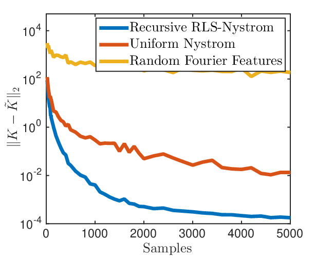
Figure 2: For a given number of samples, Recursive RLS-Nyström yields approximations with lower error, measured by ‖𝐊−𝐊~‖2\|\mathbf{K}-\mathbf{\tilde{K}}\|_{2}. Error is plotted on a logarithmic scale, averaged over 10 trials.

Figure 2 confirms that Recursive RLS-Nyström consistently obtains better kernel approximation error than the other methods. The advantage of Nyström over random Fourier features is substantial – this is unsurprising as the Nyström methods are data dependent and based on data projection, as opposed to pointwise approximation of 𝐊\mathbf{K}. Even between the Nyström methods there is a substantial difference in kernel approximation, especially for large sample sizes.

As we can see in Figure 3, with the exception of YearPredictionMSD, the better quality of the landmarks obtained with Recursive RLS-Nyström translates into runtime improvements. While the cost per sample is higher for our method at O⁡(n​d+n​s)O(nd+ns) time versus O⁡(n​d+s2)O(nd+s^{2}) for uniform Nyström and O⁡(n​d)O(nd) for random Fourier features, since RLS-Nyström requires fewer samples it more quickly obtains 𝐊~\mathbf{\tilde{K}} with a given accuracy. 𝐊~\mathbf{\tilde{K}} will also have lower rank, which can accelerate processing in downstream applications. For example, to achieve ‖𝐊−𝐊~‖2≤1\|\mathbf{K}-\mathbf{\tilde{K}}\|_{2}\leq 1 for the Covertype dataset, Recursive RLS-Nyström requires 650 samples in comparison to 3800 for uniform Nyström.

Refer to caption
(a) Adult
Refer to caption
(b) Covertype
Refer to caption
(c) Cod-RNA
Refer to caption
(d) YearPredictionMSD
Figure 3: Especially for small error, Recursive RLS-Nyström typically obtains a fixed level of approximation faster than uniform sampling. It only underperformed uniform sampling for the YearPredictionMSD dataset. Results for random Fourier features are excluded from this plot: while the method is faster than Nyström, it never obtained high enough accuracy to be directly comparable. Error is plotted on a log scale, with results averaged over 10 trials.

5.2.1 Accelerated recursive method

While Recursive RLS-Nyström typically outperforms classic Nyström, on datasets with relatively uniform ridge leverage scores, such as YearPredictionMSD, it only narrowly beats uniform sampling in terms accuracy. As a result it incurs a higher runtime cost since it is slower per sample.

To combat this issue we implement a simple heuristic modification of our algorithm. We note that the final cost of computing the Nyström factors 𝐊𝐒\mathbf{KS} and (𝐒T​𝐊𝐒)+(\mathbf{S}^{T}\mathbf{K}\mathbf{S})^{+} is O⁡(n​s+s3)O(ns+s^{3}) for both methods. Recursive RLS-Nyström is only slower because computing leverage scores at intermediate levels of recursion takes O⁡(n​s2)O(ns^{2}) time (Step 9, Algorithm 3) . This cost can be improved by simply adjusting the regularization λ\lambda to restrict the sample size on each recursive call to be <s<s. Specifically, we can balance runtimes by taking ≈(n​s+s3)/n\approx\sqrt{(ns+s^{3})/n} samples on lower levels.

Doing so improves our runtime, bringing the per sample cost down to approximately that of random Fourier features and uniform Nyström (Figure 4(a)) while nearly maintaining the same approximation quality. For datasets such as Covertype in which Recursive RLS-Nyström performs significantly better than uniform sampling, so does the accelerated method (see Figure 4(b)). However, the performance of the accelerated method does not degrade when leverage scores are relatively uniform – it still offers the best runtime to approximation quality tradeoff (Figure 4(c)).

We note that further runtime improvements may be possible. Subsequent work extends fast ridge leverage score methods to distributed and streaming environments [CLV17]. Empirical evaluation of these techniques could lead to even more scalable, high accuracy Nyström methods.

Refer to caption
(a) Runtimes for Covertype.
Refer to caption
(b) Errors for Covertype.
Refer to caption
(c) Runtime/error tradeoff for YearPredictionMSD.
Figure 4: Our accelerated Recursive RLS-Nyström, which undersamples at intermediate recursive calls, nearly matches the per sample runtime of random Fourier features and uniform Nyström while still providing approximation nearly as good as the standard Recursive RLS-Nyström. For datasets like YearPredictionMSD with relatively uniform kernel leverage scores, the accelerated version offers the best runtime vs. approximation tradeoff. All results are averaged over 10 trials.

5.3 Performance of Recursive RLS-Nyström for learning tasks

Refer to caption
(a) Covertype
Refer to caption
(b) YearPredictionMSD
Figure 5: Performance of kernel approximation methods for classification and clustering. For Covertype, classification error is measured in separating Class 2 from the remaining classes. For YearPredictionMSD, RMSE is for the unnormalized output. Regularization and kernel parameters are obtained via cross validation on training data. Test results are averaged over 10 trials with a fixed test set, as all three algorithms are randomized.

We conclude by verifying the usefulness of our kernel approximations in downstream learning tasks. We focus on Covertype and YearPredictionMSD, which each have approximately n=500,000n=500,000 data points. While full kernel methods do not scale in this regime, Recursive RLS-Nyström does since its runtime depends linearly on nn. For example, on YearPredictionMSD the method requires 307307 sec. (averaged over 55 trials) to build a 2,0002,000 landmark Nyström approximation for 463,716463,716 training points. Ridge regression using the approximate kernel then requires 208208 sec. for a total of 515515 sec. In comparison, the fastest method, random Fourier features, required 4343 sec. to build a rank 2,0002,000 kernel approximation and 222222 sec. for regression, for a total time of 265265 sec.

For Covertype we performed classification using the LIBLINEAR support vector machine library. For all sample sizes the SVM dominated runtime cost, so Recursive RLS-Nyström was only marginally slower than uniform Nyström and random Fourier features for a fixed sample size.

In terms of classification rate for Covertype and RMSE error for YearPredictionMSD, as can be seen in Figure 5, both Nyström methods outperform random features. However, we do not see much difference between the two Nyström methods. We leave open understanding why the significantly better kernel approximations discussed in Section 5.2 do not necessarily translate to much better learning performance, or whether they would make a larger difference for other problems.

Acknowledgements

We would like to thank Michael Mahoney for bringing the potential of ridge leverage scores to our attention and suggesting their possible approximation via iterative sampling schemes. We would also like to thank Michael Cohen for pointing out (and fixing) an error in our original manuscript and generally for his close collaboration in our work on leverage score sampling algorithms. Finally, thanks to Haim Avron for pointing our an error in our original analysis.

References

  • [AM15] Ahmed Alaoui and Michael W Mahoney. Fast randomized kernel ridge regression with statistical guarantees. In Advances in Neural Information Processing Systems 28 (NIPS), pages 775–783, 2015.
  • [AMS01] Dimitris Achlioptas, Frank Mcsherry, and Bernhard Schölkopf. Sampling techniques for kernel methods. In Advances in Neural Information Processing Systems 14 (NIPS), 2001.
  • [ANW14] Haim Avron, Huy Nguyen, and David Woodruff. Subspace embeddings for the polynomial kernel. In Advances in Neural Information Processing Systems 27 (NIPS), pages 2258–2266, 2014.
  • [Bac13] Francis Bach. Sharp analysis of low-rank kernel matrix approximations. In Proceedings of the 26th Annual Conference on Computational Learning Theory (COLT), 2013.
  • [BBV06] Maria-Florina Balcan, Avrim Blum, and Santosh Vempala. Kernels as features: On kernels, margins, and low-dimensional mappings. Machine Learning, 65(1):79–94, 2006.
  • [BJ02] Francis Bach and Michael I. Jordan. Kernel independent component analysis. Journal of Machine Learning Research, 3(Jul):1–48, 2002.
  • [BMD09] Christos Boutsidis, Michael W. Mahoney, and Petros Drineas. Unsupervised feature selection for the kk-means clustering problem. In Advances in Neural Information Processing Systems 22 (NIPS), pages 153–161, 2009.
  • [BW09] Mohamed-Ali Belabbas and Patrick J. Wolfe. Spectral methods in machine learning: New strategies for very large datasets. Proceedings of the National Academy of Sciences of the USA, 106:369–374, 2009.
  • [BWZ16] Christos Boutsidis, David P. Woodruff, and Peilin Zhong. Optimal principal component analysis in distributed and streaming models. In Proceedings of the 48th Annual ACM Symposium on Theory of Computing (STOC), 2016.
  • [CEM+15] Michael B. Cohen, Sam Elder, Cameron Musco, Christopher Musco, and Madalina Persu. Dimensionality reduction for k-means clustering and low rank approximation. In Proceedings of the 47th Annual ACM Symposium on Theory of Computing (STOC), pages 163–172, 2015.
  • [CLL+15] Shouyuan Chen, Yang Liu, Michael Lyu, Irwin King, and Shengyu Zhang. Fast relative-error approximation algorithm for ridge regression. In Proceedings of the 31st Annual Conference on Uncertainty in Artificial Intelligence (UAI), pages 201–210, 2015.
  • [CLM+15] Michael B. Cohen, Yin Tat Lee, Cameron Musco, Christopher Musco, Richard Peng, and Aaron Sidford. Uniform sampling for matrix approximation. In Proceedings of the 6th Conference on Innovations in Theoretical Computer Science (ITCS), pages 181–190, 2015.
  • [CLV16] Daniele Calandriello, Alessandro Lazaric, and Michal Valko. Analysis of Nyström method with sequential ridge leverage score sampling. In Proceedings of the 32nd Annual Conference on Uncertainty in Artificial Intelligence (UAI), pages 62–71, 2016.
  • [CLV17] Daniele Calandriello, Alessandro Lazaric, and Michal Valko. Distributed adaptive sampling for kernel matrix approximation. In Proceedings of the 20th International Conference on Artificial Intelligence and Statistics (AISTATS), 2017.
  • [CMM17] Michael B. Cohen, Cameron Musco, and Christopher Musco. Input sparsity time low-rank approximation via ridge leverage score sampling. In Proceedings of the 28th Annual ACM-SIAM Symposium on Discrete Algorithms (SODA), pages 1758–1777, 2017.
  • [CW17] Kenneth L. Clarkson and David P. Woodruff. Low-rank PSD approximation in input-sparsity time. In Proceedings of the 28th Annual ACM-SIAM Symposium on Discrete Algorithms (SODA), pages 2061–2072, 2017.
  • [DM05] Petros Drineas and Michael W Mahoney. On the Nyström method for approximating a Gram matrix for improved kernel-based learning. Journal of Machine Learning Research, 6:2153–2175, 2005.
  • [DMIMW12] Petros Drineas, Malik Magdon-Ismail, Michael W. Mahoney, and David P. Woodruff. Fast approximation of matrix coherence and statistical leverage. Journal of Machine Learning Research, 13:3475–3506, 2012.
  • [DMM08] Petros Drineas, Michael W Mahoney, and S Muthukrishnan. Relative-error CUR matrix decompositions. SIAM Journal on Matrix Analysis and Applications, 30(2):844–881, 2008.
  • [DST03] Vin De Silva and Joshua B Tenenbaum. Global versus local methods in nonlinear dimensionality reduction. In Advances in Neural Information Processing Systems 16 (NIPS), pages 721–728, 2003.
  • [FS02] Shai Fine and Katya Scheinberg. Efficient SVM training using low-rank kernel representations. Journal of Machine Learning Research, 2:243–264, 2002.
  • [FSS13] Dan Feldman, Melanie Schmidt, and Christian Sohler. Turning big data into tiny data: Constant-size coresets for kk-means, PCA, and projective clustering. In Proceedings of the 24th Annual ACM-SIAM Symposium on Discrete Algorithms (SODA), pages 1434–1453, 2013.
  • [Git11] Alex Gittens. The spectral norm error of the naive Nyström extension. arXiv:1110.5305, 2011.
  • [GM13] Alex Gittens and Michael Mahoney. Revisiting the Nyström method for improved large-scale machine learning. In Proceedings of the 30th International Conference on Machine Learning (ICML), pages 567–575, 2013. Full version at arXiv:1303.1849.
  • [HFH+09] Mark Hall, Eibe Frank, Geoffrey Holmes, Bernhard Pfahringer, Peter Reutemann, and Ian H Witten. The WEKA data mining software: an update. ACM SIGKDD Explorations Newsletter, 11(1):10–18, 2009.
  • [HKZ14] Daniel Hsu, Sham M. Kakade, and Tong Zhang. Random design analysis of ridge regression. Foundations of Computational Mathematics, 14(3):569–600, 2014.
  • [HTF02] Trevor Hastie, Robert Tibshirani, and Jerome Friedman. The elements of statistical learning: data mining, inference and prediction. Springer, 2nd edition, 2002.
  • [IBM14] IBM Reseach Division, Skylark Team. Libskylark: Sketching-based Distributed Matrix Computations for Machine Learning. IBM Corporation, Armonk, NY, 2014.
  • [KMT12] Sanjiv Kumar, Mehryar Mohri, and Ameet Talwalkar. Sampling methods for the Nyström method. Journal of Machine Learning Research, 13:981–1006, 2012.
  • [LBKL15] Mu Li, Wei Bi, James T Kwok, and Bao-Liang Lu. Large-scale Nyström kernel matrix approximation using randomized SVD. IEEE Transactions on Neural Networks and Learning Systems, 26(1):152–164, 2015.
  • [Lic13] M. Lichman. UCI machine learning repository, 2013.
  • [LJS16] Chengtao Li, Stefanie Jegelka, and Suvrit Sra. Fast DPP sampling for Nyström with application to kernel methods. In Proceedings of the 33rd International Conference on Machine Learning (ICML), 2016.
  • [LSS13] Quoc Le, Tamás Sarlós, and Alexander Smola. Fastfood - Computing Hilbert space expansions in loglinear time. In Proceedings of the 30th International Conference on Machine Learning (ICML), pages 244–252, 2013.
  • [MU17] Michael Mitzenmacher and Eli Upfal. Probability and Computing: Randomization and Probabilistic Techniques in Algorithms and Data Analysis. Cambridge university press, 2017.
  • [PD16] Saurabh Paul and Petros Drineas. Feature selection for ridge regression with provable guarantees. Neural Computation, 28(4):716–742, 2016.
  • [Pla05] John Platt. FastMap, MetricMap, and Landmark MDS are all Nyström algorithms. In Proceedings of the 8th International Conference on Artificial Intelligence and Statistics (AISTATS), 2005.
  • [PVG+11] F. Pedregosa, G. Varoquaux, A. Gramfort, V. Michel, B. Thirion, O. Grisel, M. Blondel, P. Prettenhofer, R. Weiss, V. Dubourg, J. Vanderplas, A. Passos, D. Cournapeau, M. Brucher, M. Perrot, and E. Duchesnay. Scikit-learn: Machine learning in Python. Journal of Machine Learning Research, 12:2825–2830, 2011.
  • [RCR15] Alessandro Rudi, Raffaello Camoriano, and Lorenzo Rosasco. Less is more: Nyström computational regularization. In Advances in Neural Information Processing Systems 28 (NIPS), pages 1648–1656, 2015.
  • [RR07] Ali Rahimi and Benjamin Recht. Random features for large-scale kernel machines. In Advances in Neural Information Processing Systems 20 (NIPS), pages 1177–1184, 2007.
  • [RR09] Ali Rahimi and Benjamin Recht. Weighted sums of random kitchen sinks: Replacing minimization with randomization in learning. In Advances in Neural Information Processing Systems 22 (NIPS), pages 1313–1320, 2009.
  • [SS00] Alex J Smola and Bernhard Schökopf. Sparse greedy matrix approximation for machine learning. In Proceedings of the 17th International Conference on Machine Learning (ICML), pages 911–918, 2000.
  • [SS02] Bernhard Schölkopf and Alexander J Smola. Learning with kernels: support vector machines, regularization, optimization, and beyond. MIT press, 2002.
  • [SSM99] Bernhard Schölkopf, Alexander J. Smola, and Klaus-Robert Müller. Advances in kernel methods. chapter Kernel principal component analysis, pages 327–352. MIT Press, 1999.
  • [Tro15] Joel A. Tropp. An introduction to matrix concentration inequalities. Foundations and Trends in Machine Learning, 8(1-2):1–230, 2015.
  • [TRVR16] Stephen Tu, Rebecca Roelofs, Shivaram Venkataraman, and Benjamin Recht. Large scale kernel learning using block coordinate descent. arXiv:1602.05310, 2016.
  • [UKM06] Andrew V Uzilov, Joshua M Keegan, and David H Mathews. Detection of non-coding RNAs on the basis of predicted secondary structure formation free energy change. BMC bioinformatics, 7(1):173, 2006.
  • [Wan16] Weiran Wang. On column selection in approximate kernel canonical correlation analysis. arXiv:1602.02172, 2016.
  • [Woo14] David P. Woodruff. Sketching as a tool for numerical linear algebra. Foundations and Trends in Theoretical Computer Science, 10(1-2):1–157, 2014.
  • [WS01] Christopher Williams and Matthias Seeger. Using the Nyström method to speed up kernel machines. In Advances in Neural Information Processing Systems 14 (NIPS), pages 682–688, 2001.
  • [WZ13] Shusen Wang and Zhihua Zhang. Improving CUR matrix decomposition and the Nyström approximation via adaptive sampling. Journal of Machine Learning Research, 14:2729–2769, 2013.
  • [YLM+12] Tianbao Yang, Yu-feng Li, Mehrdad Mahdavi, Rong Jin, and Zhi-Hua Zhou. Nyström method vs random Fourier features: A theoretical and empirical comparison. In Advances in Neural Information Processing Systems 25 (NIPS), pages 476–484, 2012.
  • [YPW15] Yun Yang, Mert Pilanci, and Martin J Wainwright. Randomized sketches for kernels: Fast and optimal non-parametric regression. Annals of Statistics, 2015.
  • [YZ13] Martin Wainwright Yuchen Zhang, John Duchi. Divide and conquer kernel ridge regression. Proceedings of the 26th Annual Conference on Computational Learning Theory (COLT), 2013.
  • [Zha06] Tong Zhang. Learning bounds for kernel regression using effective data dimensionality. Learning, 17(9), 2006.
  • [ZTK08] Kai Zhang, Ivor W. Tsang, and James T. Kwok. Improved Nyström low-rank approximation and error analysis. In Proceedings of the 25th International Conference on Machine Learning (ICML), pages 1232–1239, 2008.

Appendix A Ridge leverage score sampling bounds

Here we give the primary matrix concentration results used to bound the performance of ridge leverage score sampling in Theorems 3, 7, and 10.

Lemma 11.

For any λ>0\lambda>0 and δ∈(0,1/8)\delta\in(0,1/8), given ridge leverage score approximations l~iλ≥łiλ\tilde{l}_{i}^{\lambda}\geq\l_{i}^{\lambda} for all ii, let pi=min⁡{1,16​l~iλ​log⁡(∑l~iλ/δ)}p_{i}=\min\left\{1,16\tilde{l}_{i}^{\lambda}\log(\sum\tilde{l}_{i}^{\lambda}/\delta)\right\}. Let 𝐒∈ℝn×s\mathbf{S}\in\mathbb{R}^{n\times s} be selected by sampling the standard basis vectors 𝐞1,…,𝐞n\mathbf{e}_{1},\ldots,\mathbf{e}_{n} each independently with probability pip_{i} and rescaling selected columns by 1/pi1/\sqrt{p_{i}}. With probability 1−δ1-\delta, 1/2⋅∑ipi≤s≤2​∑ipi1/2\cdot\sum_{i}p_{i}\leq s\leq 2\sum_{i}p_{i} and:

12​𝐁T​𝐁−12​λ​𝐈⪯𝐁T​𝐒𝐒T​𝐁⪯32​𝐁T​𝐁+12​λ​𝐈,\displaystyle\frac{1}{2}\mathbf{B}^{T}\mathbf{B}-\frac{1}{2}\lambda\mathbf{I}\preceq\mathbf{B}^{T}\mathbf{SS}^{T}\mathbf{B}\preceq\frac{3}{2}\mathbf{B}^{T}\mathbf{B}+\frac{1}{2}\lambda\mathbf{I}, (22)
Proof.

Let 𝐁=𝐔​𝚺​𝐕T\mathbf{B}=\mathbf{U}\mathbf{\Sigma}\mathbf{V}^{T} be the singular value decomposition of 𝐁\mathbf{B}. By Definition 1:

liλ=𝐛iT​(𝐁T​𝐁+λ​𝐈)−1​𝐛i\displaystyle l_{i}^{\lambda}=\mathbf{b}_{i}^{T}\left(\mathbf{B}^{T}\mathbf{B}+\lambda\mathbf{I}\right)^{-1}\mathbf{b}_{i} =𝐛iT​(𝐕​𝚺2​𝐕T+λ​𝐕𝐕T)−1​𝐛i\displaystyle=\mathbf{b}_{i}^{T}\left(\mathbf{V}\mathbf{\Sigma}^{2}\mathbf{V}^{T}+\lambda\mathbf{V}\mathbf{V}^{T}\right)^{-1}\mathbf{b}_{i}
=𝐛iT​(𝐕​𝚺¯2​𝐕T)−1​𝐛i\displaystyle=\mathbf{b}_{i}^{T}\left(\mathbf{V}\mathbf{\bar{\Sigma}}^{2}\mathbf{V}^{T}\right)^{-1}\mathbf{b}_{i}
=𝐛iT​(𝐕​𝚺¯−2​𝐕T)​𝐛i,\displaystyle=\mathbf{b}_{i}^{T}\left(\mathbf{V}\mathbf{\bar{\Sigma}}^{-2}\mathbf{V}^{T}\right)\mathbf{b}_{i},

where 𝚺¯i,i2=σi2​(𝐁)+λ\mathbf{\bar{\Sigma}}^{2}_{i,i}=\sigma^{2}_{i}(\mathbf{B})+\lambda. For each i∈1,…,ni\in 1,\ldots,n define the matrix valued random variable:

𝐗i={(1pi−1)​𝚺¯−1​𝐕T​𝐛i​𝐛iT​𝐕​𝚺¯−1​ with probability ​pi−𝚺¯−1​𝐕T​𝐛i​𝐛iT​𝐕​𝚺¯−1​ with probability ​(1−pi)\displaystyle\mathbf{X}_{i}=\begin{cases}\left(\frac{1}{p_{i}}-1\right)\mathbf{\bar{\Sigma}}^{-1}\mathbf{V}^{T}\mathbf{b}_{i}\mathbf{b}_{i}^{T}\mathbf{V}\mathbf{\bar{\Sigma}}^{-1}\text{ with probability }p_{i}\\ -\mathbf{\bar{\Sigma}}^{-1}\mathbf{V}^{T}\mathbf{b}_{i}\mathbf{b}_{i}^{T}\mathbf{V}\mathbf{\bar{\Sigma}}^{-1}\text{ with probability }(1-p_{i})\end{cases}

Let 𝐘=∑i𝐗i\mathbf{Y}=\sum_{i}\mathbf{X}_{i}. We have 𝔼𝐘=𝟎\E\mathbf{Y}=\mathbf{0}. Furthermore, 𝐁T​𝐒𝐒T​𝐁=𝐕​𝚺¯​𝐘​𝚺¯​𝐕T+𝐁T​𝐁\mathbf{B}^{T}\mathbf{S}\mathbf{S}^{T}\mathbf{B}=\mathbf{V}\mathbf{\bar{\Sigma}}\mathbf{Y}\mathbf{\bar{\Sigma}}\mathbf{V}^{T}+\mathbf{B}^{T}\mathbf{B}. If we can show that ‖𝐘‖2≤12\|\mathbf{Y}\|_{2}\leq\frac{1}{2}, then since 𝐕​𝚺¯2​𝐕T=𝐁T​𝐁+λ​𝐈\mathbf{V}\mathbf{\bar{\Sigma}}^{2}\mathbf{V}^{T}=\mathbf{B}^{T}\mathbf{B}+\lambda\mathbf{I} this would give the desired bound:

12​𝐁T​𝐁−12​λ​𝐈⪯𝐁T​𝐒𝐒T​𝐁⪯32​𝐁T​𝐁+12​λ​𝐈.\displaystyle\frac{1}{2}\mathbf{B}^{T}\mathbf{B}-\frac{1}{2}\lambda\mathbf{I}\preceq\mathbf{B}^{T}\mathbf{SS}^{T}\mathbf{B}\preceq\frac{3}{2}\mathbf{B}^{T}\mathbf{B}+\frac{1}{2}\lambda\mathbf{I}.

To prove that ‖𝐘‖2\|\mathbf{Y}\|_{2} is small we use an intrinsic dimension matrix Bernstein inequality. This inequality will bound the deviation of 𝐘\mathbf{Y} from its expectation as long as we can bound each ‖𝐗i‖2\|\mathbf{X}_{i}\|_{2} and we can bound the matrix variance 𝔼(𝐘2)\E(\mathbf{Y}^{2}).

Theorem 12 (Theorem 7.3.1, [Tro15]).

Let 𝐗1,…,𝐗n\mathbf{X}_{1},\ldots,\mathbf{X}_{n} be random symmetric matrices such that for all ii, 𝔼𝐗=𝟎\E\mathbf{X}=\mathbf{0} and ‖𝐗i‖2≤L\|\mathbf{X}_{i}\|_{2}\leq L. Let 𝐘=∑i=1n𝐗i\mathbf{Y}=\sum_{i=1}^{n}\mathbf{X}_{i}. As long we can bound the matrix variance:

𝔼(𝐘2)⪯𝐙,\displaystyle\E(\mathbf{Y}^{2})\preceq\mathbf{Z},

then for for t≥‖𝐙‖2+L/3t\geq\sqrt{\|\mathbf{Z}\|_{2}}+L/3,

ℙ[∥𝐘∥≥t]\displaystyle\Pr\left[\|\mathbf{Y}\|\geq t\right] ≤4​tr⁡(𝐙)‖𝐙‖2​e−t2/2‖𝐙‖2+L​t/3.\displaystyle\leq 4\frac{\tr(\mathbf{Z})}{\|\mathbf{Z}\|_{2}}e^{\frac{-t^{2}/2}{\|\mathbf{Z}\|_{2}+Lt/3}}.

If pi=1p_{i}=1 (i.e. c​l~iλ​log⁡(∑liλ~/δ)≥1c\tilde{l}_{i}^{\lambda}\log(\sum l_{i}^{\tilde{\lambda}}/\delta)\geq 1) then 𝐗i=𝟎\mathbf{X}_{i}=\mathbf{0} so ‖𝐗i‖2=0\|\mathbf{X}_{i}\|_{2}=0. Otherwise, we use the fact that:

1l~iλ​𝐛i​𝐛iT⪯1liλ​𝐛i​𝐛iT⪯𝐁T​𝐁+λ​𝐈.\displaystyle\frac{1}{\tilde{l}_{i}^{\lambda}}\mathbf{b}_{i}\mathbf{b}_{i}^{T}\preceq\frac{1}{l_{i}^{\lambda}}\mathbf{b}_{i}\mathbf{b}_{i}^{T}\preceq\mathbf{B}^{T}\mathbf{B}+\lambda\mathbf{I}. (23)

This follows because we can write any 𝐱\mathbf{x} as 𝐱=(𝐁T𝐁+λ𝐈)−1/2𝐲\mathbf{x}=(\mathbf{B}^{T}\mathbf{B}+\lambda\mathbf{I})^{-1/2}\mathbf{y} for some 𝐲\mathbf{y}. We can then write:

𝐱T​𝐛i​𝐛iT​𝐱\displaystyle\mathbf{x}^{T}\mathbf{b}_{i}\mathbf{b}_{i}^{T}\mathbf{x} =𝐲T(𝐁T𝐁+λ𝐈)−1/2𝐛i𝐛iT(𝐁T𝐁+λ𝐈)−1/2𝐲\displaystyle=\mathbf{y}^{T}(\mathbf{B}^{T}\mathbf{B}+\lambda\mathbf{I})^{-1/2}\mathbf{b}_{i}\mathbf{b}_{i}^{T}(\mathbf{B}^{T}\mathbf{B}+\lambda\mathbf{I})^{-1/2}\mathbf{y}
≤∥𝐲∥22⋅∥(𝐁T𝐁+λ𝐈)−1/2𝐛i𝐛iT(𝐁T𝐁+λ𝐈)−1/2∥2.\displaystyle\leq\|\mathbf{y}\|_{2}^{2}\cdot\|(\mathbf{B}^{T}\mathbf{B}+\lambda\mathbf{I})^{-1/2}\mathbf{b}_{i}\mathbf{b}_{i}^{T}(\mathbf{B}^{T}\mathbf{B}+\lambda\mathbf{I})^{-1/2}\|_{2}.

Since (𝐁T𝐁+λ𝐈)−1/2𝐛i𝐛iT(𝐁T𝐁+λ𝐈)−1/2(\mathbf{B}^{T}\mathbf{B}+\lambda\mathbf{I})^{-1/2}\mathbf{b}_{i}\mathbf{b}_{i}^{T}(\mathbf{B}^{T}\mathbf{B}+\lambda\mathbf{I})^{-1/2} is rank 11, we have:

∥(𝐁T𝐁+λ𝐈)−1/2𝐛i𝐛iT(𝐁T𝐁+λ𝐈)−1/2∥2\displaystyle\|(\mathbf{B}^{T}\mathbf{B}+\lambda\mathbf{I})^{-1/2}\mathbf{b}_{i}\mathbf{b}_{i}^{T}(\mathbf{B}^{T}\mathbf{B}+\lambda\mathbf{I})^{-1/2}\|_{2} =tr((𝐁T𝐁+λ𝐈)−1/2𝐛i𝐛iT(𝐁T𝐁+λ𝐈)−1/2)\displaystyle=\tr\left((\mathbf{B}^{T}\mathbf{B}+\lambda\mathbf{I})^{-1/2}\mathbf{b}_{i}\mathbf{b}_{i}^{T}(\mathbf{B}^{T}\mathbf{B}+\lambda\mathbf{I})^{-1/2}\right)
=𝐛iT​(𝐁T​𝐁+λ​𝐈)−1​𝐛i=liλ\displaystyle=\mathbf{b}_{i}^{T}(\mathbf{B}^{T}\mathbf{B}+\lambda\mathbf{I})^{-1}\mathbf{b}_{i}=l_{i}^{\lambda} (24)

where in the last step we use the cyclic property of the trace. Writing 𝐲=(𝐁T​𝐁+λ​𝐈)1/2​𝐱\mathbf{y}=(\mathbf{B}^{T}\mathbf{B}+\lambda\mathbf{I})^{1/2}\mathbf{x} and plugging back into (24) gives:

𝐱T​𝐛i​𝐛iT​𝐱≤‖𝐲‖22⋅liλ=𝐱T​(𝐁T​𝐁+λ​𝐈)​𝐱⋅liλ.\displaystyle\mathbf{x}^{T}\mathbf{b}_{i}\mathbf{b}_{i}^{T}\mathbf{x}\leq\|\mathbf{y}\|_{2}^{2}\cdot l_{i}^{\lambda}=\mathbf{x}^{T}(\mathbf{B}^{T}\mathbf{B}+\lambda\mathbf{I})\mathbf{x}\cdot l_{i}^{\lambda}.

Rearranging and using that l~iλ≥liλ\tilde{l}_{i}^{\lambda}\geq l_{i}^{\lambda} gives (23). With this bound in place we get:

1l~iλ⋅𝚺¯−1​𝐕T​𝐛i​𝐛iT​𝐕​𝚺¯−1⪯𝚺¯−1​𝐕T​(𝐁T​𝐁+λ​𝐈)​𝐕​𝚺¯−1=𝐈.\displaystyle\frac{1}{\tilde{l}_{i}^{\lambda}}\cdot\mathbf{\bar{\Sigma}}^{-1}\mathbf{V}^{T}\mathbf{b}_{i}\mathbf{b}_{i}^{T}\mathbf{V}\mathbf{\bar{\Sigma}}^{-1}\preceq\mathbf{\bar{\Sigma}}^{-1}\mathbf{V}^{T}\left(\mathbf{B}^{T}\mathbf{B}+\lambda\mathbf{I}\right)\mathbf{V}\mathbf{\bar{\Sigma}}^{-1}=\mathbf{I}.

So we have:

𝐗i⪯1pi​𝚺¯−1​𝐕T​𝐛i​𝐛iT​𝐕​𝚺¯−1⪯l~iλpi​𝐈=116​log⁡(∑liλ~/δ)​𝐈⪯116​log⁡(∑liλ/δ)​𝐈.\displaystyle\mathbf{X}_{i}\preceq\frac{1}{p_{i}}\mathbf{\bar{\Sigma}}^{-1}\mathbf{V}^{T}\mathbf{b}_{i}\mathbf{b}_{i}^{T}\mathbf{V}\mathbf{\bar{\Sigma}}^{-1}\preceq\frac{\tilde{l}_{i}^{\lambda}}{p_{i}}\mathbf{I}=\frac{1}{16\log\left(\sum l_{i}^{\tilde{\lambda}}/\delta\right)}\mathbf{I}\preceq\frac{1}{16\log\left(\sum l_{i}^{\lambda}/\delta\right)}\mathbf{I}.

Next we bound the variance of 𝐘\mathbf{Y}.

𝔼(𝐘2)=∑𝔼(𝐗i2)\displaystyle\E(\mathbf{Y}^{2})=\sum\E(\mathbf{X}_{i}^{2}) ⪯∑[pi​(1pi−1)2+(1−pi)]⋅𝚺¯−1​𝐕T​𝐛i​𝐛iT​𝐕​𝚺¯−2​𝐕T​𝐛i​𝐛iT​𝐕​𝚺¯−1\displaystyle\preceq\sum\left[p_{i}\left(\frac{1}{p_{i}}-1\right)^{2}+(1-p_{i})\right]\cdot\mathbf{\bar{\Sigma}}^{-1}\mathbf{V}^{T}\mathbf{b}_{i}\mathbf{b}_{i}^{T}\mathbf{V}\mathbf{\bar{\Sigma}}^{-2}\mathbf{V}^{T}\mathbf{b}_{i}\mathbf{b}_{i}^{T}\mathbf{V}\mathbf{\bar{\Sigma}}^{-1}
⪯∑1pi⋅liλ~⋅𝚺¯−1​𝐕T​𝐛i​𝐛iT​𝐕​𝚺¯−1⪯116​log⁡(∑liλ/δ)​𝚺¯−1​𝐕T​𝐁T​𝐁𝐕​𝚺¯−1\displaystyle\preceq\sum\frac{1}{p_{i}}\cdot l_{i}^{\tilde{\lambda}}\cdot\mathbf{\bar{\Sigma}}^{-1}\mathbf{V}^{T}\mathbf{b}_{i}\mathbf{b}_{i}^{T}\mathbf{V}\mathbf{\bar{\Sigma}}^{-1}\preceq\frac{1}{16\log\left(\sum l_{i}^{\lambda}/\delta\right)}\mathbf{\bar{\Sigma}}^{-1}\mathbf{V}^{T}\mathbf{B}^{T}\mathbf{B}\mathbf{V}\mathbf{\bar{\Sigma}}^{-1}
⪯116​log⁡(∑liλ/δ)​𝚺2​𝚺¯−2⪯116​log⁡(∑liλ/δ)​𝐃.\displaystyle\preceq\frac{1}{16\log\left(\sum l_{i}^{\lambda}/\delta\right)}\mathbf{\Sigma}^{2}\mathbf{\bar{\Sigma}}^{-2}\preceq\frac{1}{16\log\left(\sum l_{i}^{\lambda}/\delta\right)}\mathbf{D}. (25)

where 𝐃1,1=1\mathbf{D}_{1,1}=1 and 𝐃i,i=(𝚺2​𝚺¯−2)i,i=σi2​(𝐁)σi2​(𝐁)+λ\mathbf{D}_{i,i}=(\mathbf{\Sigma}^{2}\mathbf{\bar{\Sigma}}^{-2})_{i,i}=\frac{\sigma_{i}^{2}(\mathbf{B})}{\sigma_{i}^{2}(\mathbf{B})+\lambda} for all i≥2i\geq 2. Note that ‖𝐃‖2=1\|\mathbf{D}\|_{2}=1.

Then applying Theorem 12 with 𝐙=𝐃/16​log⁡(∑liλ/δ)\mathbf{Z}=\mathbf{D}/16\log\left(\sum l_{i}^{\lambda}/\delta\right) we see that:

ℙ[∥𝐘∥2≥12]\displaystyle\Pr\left[\|\mathbf{Y}\|_{2}\geq\frac{1}{2}\right] ≤4​tr⁡(𝐃)​e−1/8116​log⁡(∑liλ/δ)+1192​log⁡(∑liλ/δ).\displaystyle\leq 4\tr(\mathbf{D})e^{\frac{-1/8}{\frac{1}{16\log(\sum l_{i}^{\lambda}/\delta)}+\frac{1}{192\log(\sum l_{i}^{\lambda}/\delta)}}}. (26)

Then we observe that:

tr⁡(𝐃)≤1+tr⁡(𝚺2​𝚺¯−2)=1+tr⁡(𝐊​(𝐊+λ​𝐈)−1)=1+∑iliλ.\displaystyle\tr(\mathbf{D})\leq 1+\tr(\mathbf{\Sigma}^{2}\mathbf{\bar{\Sigma}}^{-2})=1+\tr\left(\mathbf{K}(\mathbf{K}+\lambda\mathbf{I})^{-1}\right)=1+\sum_{i}l_{i}^{\lambda}.

Plugging into (26), establishes (27):

ℙ[∥𝐘∥≥12]\displaystyle\Pr\left[\|\mathbf{Y}\|\geq\frac{1}{2}\right] ≤4​(1+∑iliλ)⋅e−2​log⁡(∑liλ/δ)≤δ/2.\displaystyle\leq 4\left(1+\sum_{i}l_{i}^{\lambda}\right)\cdot e^{-2\log(\sum l_{i}^{\lambda}/\delta)}\leq\delta/2.

Note that here we make the extremely mild assumption that ∑iliλ≥1\sum_{i}l_{i}^{\lambda}\geq 1. If not, we can simply use a smaller λ\lambda that makes this condition true, and will have s=O⁡(1)s=O(1).

All that remains to show is that the sample size ss is bounded with high probability. If pi=1p_{i}=1, we always sample ii so there is no variance in ss. Let S⊆[1,…,n]S\subseteq[1,...,n] be the set of indices with pi<1p_{i}<1. The expected number of points sampled from SS is ∑i∈Spi=16​log⁡(∑l~iλ/δ)​∑i∈Sl~iλ\sum_{i\in S}p_{i}=16\log(\sum\tilde{l}_{i}^{\lambda}/\delta)\sum_{i\in S}\tilde{l}_{i}^{\lambda}. Assume without loss of generality that ∑i∈Sl~iλ≥1\sum_{i\in S}\tilde{l}_{i}^{\lambda}\geq 1 – otherwise can just increase our leverage score estimates and increase the expected sample size by at most 11. Then, by a standard Chernoff bound, with probability at least 1−δ/21-\delta/2,

12⋅16log(∑l~iλ/δ)∑i∈Sl~iλ≤s≤2⋅16log(∑l~iλ/δ)∑i∈Sl~iλ.\frac{1}{2}\cdot 16\log(\sum\tilde{l}_{i}^{\lambda}/\delta)\sum_{i\in S}\tilde{l}_{i}^{\lambda}\leq s\leq 2\cdot 16\log(\sum\tilde{l}_{i}^{\lambda}/\delta)\sum_{i\in S}\tilde{l}_{i}^{\lambda}.

Union bounding over failure probabilities gives the lemma. ∎

Lemma 11 yields an easy corollary about sampling without rescaling the columns in 𝐒\mathbf{S}:

Corollary 13.

For any λ>0\lambda>0 and δ∈(0,1/8)\delta\in(0,1/8), given ridge leverage score approximations l~iλ≥łiλ\tilde{l}_{i}^{\lambda}\geq\l_{i}^{\lambda} for all ii, let pi=min⁡{16​l~iλ​log⁡(∑l~iλ/δ),1}p_{i}=\min\left\{16\tilde{l}_{i}^{\lambda}\log(\sum\tilde{l}_{i}^{\lambda}/\delta),1\right\}. Let 𝐒∈ℝn×s\mathbf{S}\in\mathbb{R}^{n\times s} be selected by sampling, but not rescaling, the standard basis vectors 𝐞1,…,𝐞n\mathbf{e}_{1},\ldots,\mathbf{e}_{n} each independently with probability pip_{i}. With probability 1−δ1-\delta, 1/2⋅∑ipi≤s≤2​∑ipi1/2\cdot\sum_{i}p_{i}\leq s\leq 2\sum_{i}p_{i} and there exists some scaling factor C>0C>0 such that

𝐁T​𝐁⪯C⋅𝐁T​𝐒𝐒T​𝐁+λ​𝐈.\displaystyle\mathbf{B}^{T}\mathbf{B}\preceq C\cdot\mathbf{B}^{T}\mathbf{S}\mathbf{S}^{T}\mathbf{B}+\lambda\mathbf{I}. (27)
Proof.

By Lemma 11, if we set C′=1mini⁡piC^{\prime}=\frac{1}{\min_{i}p_{i}} we have:

12​𝐁T​𝐁−12​λ​𝐈\displaystyle\frac{1}{2}\mathbf{B}^{T}\mathbf{B}-\frac{1}{2}\lambda\mathbf{I} ⪯C′⋅𝐁T​𝐒𝐒T​𝐁\displaystyle\preceq C^{\prime}\cdot\mathbf{B}^{T}\mathbf{S}\mathbf{S}^{T}\mathbf{B}
𝐁T​𝐁\displaystyle\mathbf{B}^{T}\mathbf{B} ⪯2​C′⋅𝐁T​𝐒𝐒T​𝐁+λ​𝐈\displaystyle\preceq 2C^{\prime}\cdot\mathbf{B}^{T}\mathbf{S}\mathbf{S}^{T}\mathbf{B}+\lambda\mathbf{I}

which gives the corollary by setting C=2​C′C=2C^{\prime}. ∎

Appendix B Projection-cost preserving kernel approximation

In addition to the basic spectral approximation guarantee of Theorem 3, we prove that, with high probability, the RLS-Nyström method presented in Algorithm 1 outputs an approximation 𝐊~\mathbf{\tilde{K}} satisfying what is known as a projection-cost preservation guarantee. This approximation also immediately holds for the efficient implementation of sampling in Algorithm 3.

Theorem 14 (Projection-cost preserving kernel approximation).

Let λ=ϵk​∑i=k+1nσi​(𝐊)\lambda=\frac{\epsilon}{k}\sum_{i=k+1}^{n}\sigma_{i}(\mathbf{K}). For any ϵ∈(0,1),δ∈(0,1/8)\epsilon\in(0,1),\delta\in(0,1/8), RLS-Nyström returns an 𝐒∈ℝn×s\mathbf{S}\in\mathbb{R}^{n\times s} such that with probability 1−δ1-\delta, 1/2∑ipi≤s≤2∑ipi1/2\sum_{i}p_{i}\leq s\leq 2\sum_{i}p_{i} and the approximation 𝐊~=𝐊𝐒​(𝐒𝐊𝐒)+​𝐒𝐊\mathbf{\tilde{K}}=\mathbf{KS}(\mathbf{S}\mathbf{K}\mathbf{S})^{+}\mathbf{S}\mathbf{K} satisfies, for any rank kk orthogonal projection 𝐗\mathbf{X} and a positive constant cc independent of 𝐗\mathbf{X}:

tr⁡(𝐊−𝐗𝐊𝐗)≤tr⁡(𝐊~−𝐗​𝐊~​𝐗)+c≤(1+ϵ)​tr⁡(𝐊−𝐗𝐊𝐗).\displaystyle\tr(\mathbf{K}-\mathbf{X}\mathbf{K}\mathbf{X})\leq\tr(\mathbf{\tilde{K}}-\mathbf{X}\mathbf{\tilde{K}}\mathbf{X})+c\leq(1+\epsilon)\tr(\mathbf{K}-\mathbf{X}\mathbf{K}\mathbf{X}). (28)

When ridge leverage scores are computed exactly, ∑ipi=O⁡(kϵ​log⁡kδ​ϵ)\sum_{i}p_{i}=O\left(\frac{k}{\epsilon}\log\frac{k}{\delta\epsilon}\right).

Intuitively, Theorem 14 ensures that the distance from 𝐊~\mathbf{\tilde{K}} to any low dimensional subspace closely approximates the distance from 𝐊\mathbf{K} to the subspace. Accordingly, 𝐊~\mathbf{\tilde{K}} can be used in place of 𝐊\mathbf{K} to approximately solve low-rank approximation problems, both constrained (e.g. kk-means clustering) and unconstrained (e.g. principal component analysis). See Theorems 16 and 17.

Proof.

Set c=tr⁡(𝐊)−tr⁡(𝐊~)c=\tr(\mathbf{K})-\tr(\mathbf{\tilde{K}}), which is ≥0\geq 0 since 𝐊~⪯𝐊\mathbf{\tilde{K}}\preceq\mathbf{K} by Theorem 3. By linearity of trace:

tr⁡(𝐊~−𝐗​𝐊~​𝐗)+c=tr⁡(𝐊)−tr⁡(𝐗​𝐊~​𝐗).\displaystyle\tr(\mathbf{\tilde{K}}-\mathbf{X}\mathbf{\tilde{K}}\mathbf{X})+c=\tr(\mathbf{K})-\tr(\mathbf{X}\mathbf{\tilde{K}}\mathbf{X}).

So to obtain (28) it suffices to show:

tr⁡(𝐗𝐊𝐗)−ϵ​tr⁡(𝐊−𝐗𝐊𝐗)≤tr⁡(𝐗​𝐊~​𝐗)≤tr⁡(𝐗𝐊𝐗).\displaystyle\tr(\mathbf{X}\mathbf{K}\mathbf{X})-\epsilon\tr(\mathbf{K}-\mathbf{X}\mathbf{K}\mathbf{X})\leq\tr(\mathbf{X}\mathbf{\tilde{K}}\mathbf{X})\leq\tr(\mathbf{X}\mathbf{K}\mathbf{X}). (29)

Since 𝐗\mathbf{X} is a rank kk orthogonal projection we can write 𝐗=𝐐𝐐T\mathbf{X}=\mathbf{Q}\mathbf{Q}^{T} where 𝐐∈ℝn×k\mathbf{Q}\in\mathbb{R}^{n\times k} has orthonormal columns. Applying the cyclic property of the trace, and the spectral bound of Theorem 3:

tr⁡(𝐗​𝐊~​𝐗)=tr⁡(𝐐T​𝐊~​𝐐)=∑i=1k𝐪iT​𝐊~​𝐪i≤∑i=1k𝐪iT​𝐊𝐪i=tr⁡(𝐐T​𝐊𝐐)=tr⁡(𝐗𝐊𝐗).\displaystyle\tr(\mathbf{X}\mathbf{\tilde{K}}\mathbf{X})=\tr(\mathbf{Q}^{T}\mathbf{\tilde{K}}\mathbf{Q})=\sum_{i=1}^{k}\mathbf{q}_{i}^{T}\mathbf{\tilde{K}}\mathbf{q}_{i}\leq\sum_{i=1}^{k}\mathbf{q}_{i}^{T}\mathbf{K}\mathbf{q}_{i}=\tr(\mathbf{Q}^{T}\mathbf{K}\mathbf{Q})=\tr(\mathbf{X}\mathbf{K}\mathbf{X}).

This gives us the upper bound of (29). For the lower bound we apply Corollary 4:

tr⁡(𝐗​𝐊~​𝐗)=∑i=1k𝐪iT​𝐊~​𝐪i≥∑i=1k𝐪iT​𝐊𝐪i−k​ϵ​λ=tr⁡(𝐗𝐊𝐗)−k​ϵ​λ.\displaystyle\tr(\mathbf{X}\mathbf{\tilde{K}}\mathbf{X})=\sum_{i=1}^{k}\mathbf{q}_{i}^{T}\mathbf{\tilde{K}}\mathbf{q}_{i}\geq\sum_{i=1}^{k}\mathbf{q}_{i}^{T}\mathbf{K}\mathbf{q}_{i}-k\epsilon\lambda=\tr(\mathbf{X}\mathbf{K}\mathbf{X})-k\epsilon\lambda. (30)

Finally, k​ϵ​λ=ϵ​∑i=k+1nσi​(𝐊)≤ϵ​tr⁡(𝐊−𝐗𝐊𝐗)k\epsilon\lambda=\epsilon\sum_{i=k+1}^{n}\sigma_{i}(\mathbf{K})\leq\epsilon\tr(\mathbf{K}-\mathbf{X}\mathbf{K}\mathbf{X}) since tr⁡(𝐊)=∑i=1nσi​(𝐊)\tr(\mathbf{K})=\sum_{i=1}^{n}\sigma_{i}(\mathbf{K}) and tr⁡(𝐗𝐊𝐗)≤∑i=1kσi​(𝐊)\tr(\mathbf{X}\mathbf{K}\mathbf{X})\leq\sum_{i=1}^{k}\sigma_{i}(\mathbf{K}) by the Eckart-Young theorem. Plugging into (30) gives (29), completing the proof.

We conclude by showing that ss is not too large. As in the proof of Theorem 3, s≤2​∑ipis\leq 2\sum_{i}p_{i} with probability 1−δ1-\delta. When ridge leverage scores are computed exactly ∑ipi≤16​∑liλ​log⁡(∑liλ/δ)\sum_{i}p_{i}\leq 16\sum l_{i}^{\lambda}\log(\sum l_{i}^{\lambda}/\delta).

∑iliλ\displaystyle\sum_{i}l_{i}^{\lambda} =tr⁡(𝐊⁡(𝐊+ϵ​(1k​∑i=k+1nσi​(𝐊)​𝐈)−1)CLOSE\displaystyle=\tr(\mathbf{K}(\mathbf{K}+\epsilon\left(\frac{1}{k}\sum_{i=k+1}^{n}\sigma_{i}(\mathbf{K}\right)\mathbf{I})^{-1})
≤1ϵ​tr⁡(𝐊⁡(𝐊+(1k​∑i=k+1nσi​(𝐊)​𝐈)−1)CLOSE\displaystyle\leq\frac{1}{\epsilon}\tr(\mathbf{K}(\mathbf{K}+\left(\frac{1}{k}\sum_{i=k+1}^{n}\sigma_{i}(\mathbf{K}\right)\mathbf{I})^{-1})
=1ϵ​∑i=1nσi​(𝐊)σi​(𝐊)+1k​∑i=k+1nσi​(𝐊)\displaystyle=\frac{1}{\epsilon}\sum_{i=1}^{n}\frac{\sigma_{i}(\mathbf{K})}{\sigma_{i}(\mathbf{K})+\frac{1}{k}\sum_{i=k+1}^{n}\sigma_{i}(\mathbf{K})}
=1ϵ​(∑i=1kσi​(𝐊)σi​(𝐊)+1k​∑i=k+1nσi​(𝐊)+∑i=k+1nσi​(𝐊)σi​(𝐊)+1k​∑i=k+1nσi​(𝐊))\displaystyle=\frac{1}{\epsilon}\left(\sum_{i=1}^{k}\frac{\sigma_{i}(\mathbf{K})}{\sigma_{i}(\mathbf{K})+\frac{1}{k}\sum_{i=k+1}^{n}\sigma_{i}(\mathbf{K})}+\sum_{i=k+1}^{n}\frac{\sigma_{i}(\mathbf{K})}{\sigma_{i}(\mathbf{K})+\frac{1}{k}\sum_{i=k+1}^{n}\sigma_{i}(\mathbf{K})}\right)
≤1ϵ​(k+∑i=k+1nσi​(𝐊)1k​∑i=k+1nσi​(𝐊))=2​kϵ.\displaystyle\leq\frac{1}{\epsilon}\left(k+\sum_{i=k+1}^{n}\frac{\sigma_{i}(\mathbf{K})}{\frac{1}{k}\sum_{i=k+1}^{n}\sigma_{i}(\mathbf{K})}\right)=\frac{2k}{\epsilon}. (31)

Accordingly, ∑ipi=32​kϵ​log⁡kδ​ϵ\sum_{i}p_{i}=32\frac{k}{\epsilon}\log\frac{k}{\delta\epsilon} as desired. ∎

Appendix C Applications to learning tasks

In this section use our general approximation gaurantees from Theorems 3 and 14 to prove that the kernel approximations given by RLS-Nyström sampling are sufficient for many downstream learning tasks. In other words, 𝐊~\mathbf{\tilde{K}} can be used in place of 𝐊\mathbf{K} without sacrificing accuracy or statistical performance in the final computation.

C.1 Kernel ridge regression

We begin with a standard formulation of the ubiquitous kernel ridge regression task [SS02]. Given input data points 𝐱1,…,𝐱n∈ℝd\mathbf{x}_{1},\ldots,\mathbf{x}_{n}\in\mathbb{R}^{d} and labels y1,…,yn∈ℝy_{1},\ldots,y_{n}\in\mathbb{R} this problem asks us to solve:

𝜶=defarg​min𝐜∈ℝn⁡‖𝐊𝐜−𝐲‖22+λ​𝐜T​𝐊𝐜,\displaystyle\boldsymbol{\alpha}\mathbin{\stackrel{{\scriptstyle\rm def}}{{=}}}\argmin_{\mathbf{c}\in\mathbb{R}^{n}}\|\mathbf{K}\mathbf{c}-\mathbf{y}\|_{2}^{2}+\lambda\mathbf{c}^{T}\mathbf{K}\mathbf{c}, (32)

which can be done in closed form by computing:

𝜶=(𝐊+λ​𝐈)−1​𝐲.\displaystyle\boldsymbol{\alpha}=(\mathbf{K}+\lambda\mathbf{I})^{-1}\mathbf{y}.

For prediction, when we’re given a new input 𝐱\mathbf{x}, we evaluate its label to be:

y=∑i=1nαi​K​(𝐱i,𝐱).\displaystyle y=\sum_{i=1}^{n}\mathbf{\alpha}_{i}K(\mathbf{x}_{i},\mathbf{x}). (33)

C.1.1 Approximate kernel ridge regression

Naively, solving for 𝜶\boldsymbol{\alpha} exactly requires at least O⁡(n2)O(n^{2}) time to compute 𝐊\mathbf{K}, plus the cost of a direct or iterative matrix inversion algorithm. Prediction is also costly since it requires a kernel evaluation with all nn training points. These costs can be reduced significantly using Nyström approximation.

In particular, we first select landmark points and compute the kernel approximation 𝐊~=𝐊𝐒​(𝐒T​𝐊𝐒)+​𝐒T​𝐊\mathbf{\tilde{K}}=\mathbf{KS}(\mathbf{S}^{T}\mathbf{KS})^{+}\mathbf{S}^{T}\mathbf{K}. We can then compute an approximate set of coefficients:

𝜶~=def(𝐊~+λ​𝐈)−1​𝐲.\displaystyle\boldsymbol{\tilde{\alpha}}\mathbin{\stackrel{{\scriptstyle\rm def}}{{=}}}(\mathbf{\tilde{K}}+\lambda\mathbf{I})^{-1}\mathbf{y}. (34)

With a direct matrix inversion, doing so only takes O⁡(n​s2)O(ns^{2}) time when our sampling matrix 𝐒∈ℝn×s\mathbf{S}\in\mathbb{R}^{n\times s} selects ss landmark points. This is a significant improvement on the O⁡(n3)O(n^{3}) time required to invert the full kernel. Additionally, the cost of multiplying by 𝐊~+λ​𝐈\mathbf{\tilde{K}}+\lambda\mathbf{I}, which determines the cost of most iterative regression solvers, is reduced, from O⁡(n2)O(n^{2}) to O⁡(n​s)O(ns).

To predict a label for a new 𝐱\mathbf{x}, we first compute its kernel product with all of our landmark points. Specifically, let 𝐱(1),…,𝐱(s)\mathbf{x}^{(1)},\ldots,\mathbf{x}^{(s)} be the landmarks selected by 𝐒\mathbf{S}’s columns. Define 𝐰∈ℝs\mathbf{w}\in\mathbb{R}^{s} as:

𝐰i=defK⁡(𝐱(i),𝐱).\displaystyle\mathbf{w}_{i}\mathbin{\stackrel{{\scriptstyle\rm def}}{{=}}}K(\mathbf{x}^{(i)},\mathbf{x}).

and let

y=𝐰T​(𝐒T​𝐊𝐒)+​𝐒T​𝐊​𝜶~.\displaystyle y=\mathbf{w}^{T}(\mathbf{S}^{T}\mathbf{KS})^{+}\mathbf{S}^{T}\mathbf{K}\boldsymbol{\tilde{\alpha}}. (35)

Computationally, it makes sense to precompute (𝐒T​𝐊𝐒)+​𝐒T​𝐊​𝜶~(\mathbf{S}^{T}\mathbf{KS})^{+}\mathbf{S}^{T}\mathbf{K}\boldsymbol{\tilde{\alpha}}. Then the cost of prediction is just ss kernel evaluations to compute 𝐰\mathbf{w}, plus ss additional operations to multiply 𝐰T\mathbf{w}^{T} by (𝐒T​𝐊𝐒)+​𝐒T​𝐊​𝜶~(\mathbf{S}^{T}\mathbf{KS})^{+}\mathbf{S}^{T}\mathbf{K}\boldsymbol{\tilde{\alpha}}.

This approach is the standard way of applying Nyström approximation to the ridge regression problem and there are a number of ways to evaluate its performance. Beyond directly bounding minimization error for (32) (see e.g. [CLL+15, YPW15, YZ13]), one particularly natural approach is to consider how the statistical risk of the estimator output by our approximate ridge regression routine compares to that of the exactly computed estimator.

C.1.2 Relative error bound on statistical risk

To evaluate statistical risk we consider a fixed design setting which has been especially -popular [Bac13, AM15, LJS16, PD16]. Note that more complex statistical models can be analyzed as well [HKZ14, RCR15]. In this setting, we assume that our observed labels 𝐲=[y1,…,yn]\mathbf{y}=[y_{1},\ldots,y_{n}] represent underlying true labels 𝐳=[z1,…,zn]\mathbf{z}=[z_{1},\ldots,z_{n}] perturbed with noise. For simplicity, we assume uniform Gaussian noise with variance σ2\sigma^{2}, but more general noise models can be handled with essentially the same proof [Bac13]. In particular, our modeling assumption is that:

yi=zi+ηi\displaystyle y_{i}=z_{i}+\eta_{i}

where ηi∼N⁡(0,σ2)\eta_{i}\sim N(0,\sigma^{2}).

Following [Bac13] and [AM15], we want to bound the expected in sample risk of our estimator for 𝐳\mathbf{z}, which is computed using the noisy measurements 𝐲=𝐳+𝜼\mathbf{y}=\mathbf{z}+\boldsymbol{\eta}. For exact kernel ridge regression, we can check from (33) that this estimator is equal to 𝐊​𝜶\mathbf{K}\boldsymbol{\alpha}. The risk ℛ\mathcal{R} is:

ℛ\displaystyle\mathcal{R} =def𝔼𝜼‖𝐊​(𝐊+λ​𝐈)−1​(𝐳+𝜼)−𝐳‖22\displaystyle\mathbin{\stackrel{{\scriptstyle\rm def}}{{=}}}\E_{\boldsymbol{\eta}}\|\mathbf{K}(\mathbf{K}+\lambda\mathbf{I})^{-1}(\mathbf{z}+\boldsymbol{\eta})-\mathbf{z}\|_{2}^{2}
=‖(𝐊​(𝐊+λ​𝐈)−1−𝐈)​𝐳‖22+𝔼𝜼‖𝐊​(𝐊+λ​𝐈)−1​𝜼‖22\displaystyle=\|\left(\mathbf{K}(\mathbf{K}+\lambda\mathbf{I})^{-1}-\mathbf{I}\right)\mathbf{z}\|_{2}^{2}+\E_{\boldsymbol{\eta}}\|\mathbf{K}(\mathbf{K}+\lambda\mathbf{I})^{-1}\boldsymbol{\eta}\|_{2}^{2}
=λ2​𝐳T​(𝐊+λ​𝐈)−2​𝐳+σ2​tr⁡(𝐊2​(𝐊+λ​𝐈)−2).\displaystyle=\lambda^{2}\mathbf{z}^{T}(\mathbf{K}+\lambda\mathbf{I})^{-2}\mathbf{z}+\sigma^{2}\tr(\mathbf{K}^{2}(\mathbf{K}+\lambda\mathbf{I})^{-2}).

The two terms that compose ℛ\mathcal{R} are referred to as the bias and variance terms of the risk:

bias​(𝐊)2\displaystyle\text{bias}(\mathbf{K})^{2} =defλ2​𝐳T​(𝐊+λ​𝐈)−2​𝐳\displaystyle\mathbin{\stackrel{{\scriptstyle\rm def}}{{=}}}\lambda^{2}\mathbf{z}^{T}(\mathbf{K}+\lambda\mathbf{I})^{-2}\mathbf{z}
variance​(𝐊)\displaystyle\text{variance}(\mathbf{K}) =defσ2​tr⁡(𝐊2​(𝐊+λ​𝐈)−2).\displaystyle\mathbin{\stackrel{{\scriptstyle\rm def}}{{=}}}\sigma^{2}\tr(\mathbf{K}^{2}(\mathbf{K}+\lambda\mathbf{I})^{-2}).

For approximate kernel ridge regression, it follows from (35) that our predictor for 𝐳\mathbf{z} is 𝐊~​𝜶~\mathbf{\tilde{K}}\boldsymbol{\tilde{\alpha}}. Accordingly, the risk of the approximate estimator, ℛ~\mathcal{\tilde{R}} is equal to:

ℛ~=bias​(𝐊~)2+variance​(𝐊~)\displaystyle\mathcal{\tilde{R}}=\text{bias}(\mathbf{\tilde{K}})^{2}+\text{variance}(\mathbf{\tilde{K}})

We’re are ready to prove our main theorem on kernel ridge regression.

Theorem 15 (Kernel Ridge Regression Risk Bound).

Suppose 𝐊~\mathbf{\tilde{K}} is computed using RLS-Nyström with approximation parameter ϵ​λ\epsilon\lambda and failure probability δ∈(0,1/8)\delta\in(0,1/8). Let 𝛂~=(𝐊~+λ​𝐈)−1​𝐲\boldsymbol{\tilde{\alpha}}=(\mathbf{\tilde{K}}+\lambda\mathbf{I})^{-1}\mathbf{y} and let 𝐊~​𝛂~\mathbf{\tilde{K}}\boldsymbol{\tilde{\alpha}} be our estimator for 𝐳\mathbf{z} computed with the approximate kernel. With probability 1−δ1-\delta:

ℛ~≤(1+3​ϵ)​ℛ.\displaystyle\mathcal{\tilde{R}}\leq(1+3\epsilon)\mathcal{R}.

By Theorem 7, Algorithm 2 can compute 𝐊~\mathbf{\tilde{K}} with just O⁡(n​s)O(ns) kernel evaluations and O⁡(n​s2)O(ns^{2}) computation time, with s=O⁡(deffλϵ​log⁡deffλδ​ϵ)s=O\left(\frac{d_{\text{eff}}^{\lambda}}{\epsilon}\log\frac{d_{\text{eff}}^{\lambda}}{\delta\epsilon}\right).

In other words, replacing 𝐊\mathbf{K} with the approximation 𝐊~\mathbf{\tilde{K}} is provably sufficient for obtaining a 1+Θ⁡(ϵ)1+\Theta(\epsilon) quality solution to the downstream task of ridge regression.

Proof.

The proof follows that of Theorem 1 in [AM15]. First we show that:

bias​(𝐊~)≤(1+ϵ)​bias​(𝐊).\displaystyle\text{bias}(\mathbf{\tilde{K}})\leq(1+\epsilon)\text{bias}(\mathbf{K}). (36)

At first glance this might appear trivial as Theorem 3 easily implies that

(𝐊~+λ​𝐈)−1⪯(1+ϵ)​(𝐊+λ​𝐈)−1\displaystyle(\mathbf{\tilde{K}}+\lambda\mathbf{I})^{-1}\preceq(1+\epsilon)(\mathbf{K}+\lambda\mathbf{I})^{-1}

However, this statement does not imply that

(𝐊~+λ​𝐈)−2⪯(1+ϵ)2​(𝐊+λ​𝐈)−2\displaystyle(\mathbf{\tilde{K}}+\lambda\mathbf{I})^{-2}\preceq(1+\epsilon)^{2}(\mathbf{K}+\lambda\mathbf{I})^{-2}

since (𝐊~+λ​𝐈)−1(\mathbf{\tilde{K}}+\lambda\mathbf{I})^{-1} and (𝐊+λ​𝐈)−1(\mathbf{K}+\lambda\mathbf{I})^{-1} do not necessarily commute. Instead we proceed:

1λ​bias​(𝐊~)\displaystyle\frac{1}{\lambda}\text{bias}(\mathbf{\tilde{K}}) =‖(𝐊~+λ​𝐈)−1​𝐳‖2\displaystyle=\|(\mathbf{\tilde{K}}+\lambda\mathbf{I})^{-1}\mathbf{z}\|_{2}
≤‖(𝐊+λ​𝐈)−1​𝐳‖2+‖(𝐊~+λ​𝐈)−1​𝐳−(𝐊+λ​𝐈)−1​𝐳‖2\displaystyle\leq\|(\mathbf{K}+\lambda\mathbf{I})^{-1}\mathbf{z}\|_{2}+\|(\mathbf{\tilde{K}}+\lambda\mathbf{I})^{-1}\mathbf{z}-(\mathbf{K}+\lambda\mathbf{I})^{-1}\mathbf{z}\|_{2} (triangle inequality)
=‖(𝐊+λ​𝐈)−1​𝐳‖2+‖(𝐊~+λ​𝐈)−1​[(𝐊+λ​𝐈)−(𝐊~+λ​𝐈)]​(𝐊+λ​𝐈)−1​𝐳‖2\displaystyle=\|(\mathbf{K}+\lambda\mathbf{I})^{-1}\mathbf{z}\|_{2}+\|(\mathbf{\tilde{K}}+\lambda\mathbf{I})^{-1}[(\mathbf{K}+\lambda\mathbf{I})-(\mathbf{\tilde{K}}+\lambda\mathbf{I})](\mathbf{K}+\lambda\mathbf{I})^{-1}\mathbf{z}\|_{2}
=‖(𝐊+λ​𝐈)−1​𝐳‖2+‖(𝐊~+λ​𝐈)−1​(𝐊−𝐊~)​(𝐊+λ​𝐈)−1​𝐳‖2\displaystyle=\|(\mathbf{K}+\lambda\mathbf{I})^{-1}\mathbf{z}\|_{2}+\|(\mathbf{\tilde{K}}+\lambda\mathbf{I})^{-1}(\mathbf{K}-\mathbf{\tilde{K}})(\mathbf{K}+\lambda\mathbf{I})^{-1}\mathbf{z}\|_{2}
≤‖(𝐊+λ​𝐈)−1​𝐳‖2+‖(𝐊~+λ​𝐈)−1​(𝐊−𝐊~)‖2​‖(𝐊+λ​𝐈)−1​𝐳‖2\displaystyle\leq\|(\mathbf{K}+\lambda\mathbf{I})^{-1}\mathbf{z}\|_{2}+\|(\mathbf{\tilde{K}}+\lambda\mathbf{I})^{-1}(\mathbf{K}-\mathbf{\tilde{K}})\|_{2}\|(\mathbf{K}+\lambda\mathbf{I})^{-1}\mathbf{z}\|_{2} (submultiplicativity)
=1λ​bias​(𝐊)​(1+‖(𝐊~+λ​𝐈)−1​(𝐊−𝐊~)‖2).\displaystyle=\frac{1}{\lambda}\text{bias}(\mathbf{K})\left(1+\|(\mathbf{\tilde{K}}+\lambda\mathbf{I})^{-1}(\mathbf{K}-\mathbf{\tilde{K}})\|_{2}\right). (37)

So we just need to bound ‖(𝐊~+λ​𝐈)−1​(𝐊−𝐊~)‖2≤ϵ\|(\mathbf{\tilde{K}}+\lambda\mathbf{I})^{-1}(\mathbf{K}-\mathbf{\tilde{K}})\|_{2}\leq\epsilon. First note that, by Theorem 3, Corollary 4,

𝐊−𝐊~⪯ϵ​λ​𝐈\displaystyle\mathbf{K}-\mathbf{\tilde{K}}\preceq\mathbf{\epsilon}\lambda\mathbf{I}

and since (𝐊−𝐊~)(\mathbf{K}-\mathbf{\tilde{K}}) and 𝐈\mathbf{I} commute, it follows that

(𝐊−𝐊~)2⪯ϵ2​λ2​𝐈.\displaystyle(\mathbf{K}-\mathbf{\tilde{K}})^{2}\preceq\mathbf{\epsilon}^{2}\lambda^{2}\mathbf{I}. (38)

Accordingly,

‖(𝐊~+λ​𝐈)−1​(𝐊−𝐊~)‖22\displaystyle\|(\mathbf{\tilde{K}}+\lambda\mathbf{I})^{-1}(\mathbf{K}-\mathbf{\tilde{K}})\|^{2}_{2} =‖(𝐊~+λ​𝐈)−1​(𝐊−𝐊~)2​(𝐊~+λ​𝐈)−1‖2\displaystyle=\|(\mathbf{\tilde{K}}+\lambda\mathbf{I})^{-1}(\mathbf{K}-\mathbf{\tilde{K}})^{2}(\mathbf{\tilde{K}}+\lambda\mathbf{I})^{-1}\|_{2}
≤ϵ2​λ2​‖(𝐊~+λ​𝐈)−2‖2\displaystyle\leq\epsilon^{2}\lambda^{2}\|(\mathbf{\tilde{K}}+\lambda\mathbf{I})^{-2}\|_{2}
≤ϵ2​λ2​1λ2=ϵ2.\displaystyle\leq\epsilon^{2}\lambda^{2}\frac{1}{\lambda^{2}}=\epsilon^{2}.

So ‖(𝐊~+λ​𝐈)−1​(𝐊−𝐊~)‖2≤ϵ\|(\mathbf{\tilde{K}}+\lambda\mathbf{I})^{-1}(\mathbf{K}-\mathbf{\tilde{K}})\|_{2}\leq\epsilon as desired and plugging into (37) we have shown (36), that bias​(𝐊~)≤(1+ϵ)​bias​(𝐊)\text{bias}(\mathbf{\tilde{K}})\leq(1+\epsilon)\text{bias}(\mathbf{K}). We next show that:

variance​(𝐊~)≤variance​(𝐊),\displaystyle\text{variance}(\mathbf{\tilde{K}})\leq\text{variance}(\mathbf{K}), (39)

where variance​(𝐊)=σ2​tr⁡(𝐊2​(𝐊+λ​𝐈)−2)=σ2​∑i=1n(σi​(𝐊)σi​(𝐊)+λ)2\text{variance}(\mathbf{K})=\sigma^{2}\tr(\mathbf{K}^{2}(\mathbf{K}+\lambda\mathbf{I})^{-2})=\sigma^{2}\sum_{i=1}^{n}\left(\frac{\sigma_{i}(\mathbf{K})}{\sigma_{i}(\mathbf{K})+\lambda}\right)^{2}. Since 𝐊~⪯𝐊\mathbf{\tilde{K}}\preceq\mathbf{K} by Theorem 3, σi​(𝐊~)≤σi​(𝐊)\sigma_{i}(\mathbf{\tilde{K}})\leq\sigma_{i}(\mathbf{K}) for all ii. It follows that, for every ii,

σi​(𝐊~)σi​(𝐊~)+λ≤σi​(𝐊)σi​(𝐊)+λ.\displaystyle\frac{\sigma_{i}(\mathbf{\tilde{K}})}{\sigma_{i}(\mathbf{\tilde{K}})+\lambda}\leq\frac{\sigma_{i}(\mathbf{K})}{\sigma_{i}(\mathbf{K})+\lambda}.

This in turn implies that

∑i=1n(σi​(𝐊~)σi​(𝐊~)+λ)2≤∑i=1n(σi​(𝐊)σi​(𝐊)+λ)2,\displaystyle\sum_{i=1}^{n}\left(\frac{\sigma_{i}(\mathbf{\tilde{K}})}{\sigma_{i}(\mathbf{\tilde{K}})+\lambda}\right)^{2}\leq\sum_{i=1}^{n}\left(\frac{\sigma_{i}(\mathbf{K})}{\sigma_{i}(\mathbf{K})+\lambda}\right)^{2},

which gives (39). Combining (39) and (36) we conclude that, for ϵ<1\epsilon<1,

ℛ⁡(f^𝐊~)≤(1+ϵ)2​ℛ​(f^𝐊)≤(1+3​ϵ)​ℛ​(f^𝐊).\displaystyle\mathcal{R}(\hat{f}_{\mathbf{\tilde{K}}})\leq(1+\epsilon)^{2}\mathcal{R}(\hat{f}_{\mathbf{K}})\leq(1+3\epsilon)\mathcal{R}(\hat{f}_{\mathbf{K}}).

∎

C.2 Kernel kk-means

Kernel kk-means clustering asks us to partition 𝐱1,…,𝐱n\mathbf{x}_{1},\ldots,\mathbf{x}_{n}, into kk cluster sets, {C1,…,Ck}\{C_{1},\ldots,C_{k}\}. Let 𝝁i=1|Ci|​∑𝐱j∈Ciϕ⁡(𝐱j)\boldsymbol{\mu}_{i}=\frac{1}{|C_{i}|}\sum_{\mathbf{x}_{j}\in C_{i}}\phi(\mathbf{x}_{j}) be the centroid of the vectors in CiC_{i} after mapping to kernel space. The goal is to choose {C1,…,Ck}\{C_{1},\ldots,C_{k}\} which minimize the objective:

∑i=1k∑𝐱j∈Ci‖ϕ⁡(𝐱j)−𝝁i‖ℱ2\displaystyle\sum_{i=1}^{k}\sum_{\mathbf{x}_{j}\in C_{i}}\|\phi(\mathbf{x}_{j})-\boldsymbol{\mu}_{i}\|_{\mathcal{F}}^{2} (40)

It is well known that this optimization problem can be rewritten as a constrained low-rank approximation problem (see e.g. [BMD09] or [CEM+15]). In particular, for any clustering C={C1,…,Ck}C=\{C_{1},\ldots,C_{k}\} we can define a rank kk orthonormal matrix 𝐂∈ℝn×k\mathbf{C}\in\mathbb{R}^{n\times k} called the cluster indicator matrix for CC. 𝐂i,j=1/|Cj|\mathbf{C}_{i,j}=1/\sqrt{|C_{j}|} if 𝐱i\mathbf{x}_{i} is assigned to CjC_{j} and 𝐂i,j=0\mathbf{C}_{i,j}=0 otherwise. 𝐂T​𝐂=𝐈\mathbf{C}^{T}\mathbf{C}=\mathbf{I}, so 𝐂𝐂T\mathbf{C}\mathbf{C}^{T} is a rank kk projection matrix. Furthermore, it’s not hard to check that:

∑i=1k∑𝐱j∈Ci‖ϕ⁡(𝐱j)−𝝁i‖ℱ2=tr⁡(𝐊−𝐂𝐂T​𝐊𝐂𝐂T).\displaystyle\sum_{i=1}^{k}\sum_{\mathbf{x}_{j}\in C_{i}}\|\phi(\mathbf{x}_{j})-\boldsymbol{\mu}_{i}\|_{\mathcal{F}}^{2}=\tr\left(\mathbf{K}-\mathbf{C}\mathbf{C}^{T}\mathbf{K}\mathbf{C}\mathbf{C}^{T}\right). (41)

Informally, if we work with the kernalized data matrix 𝚽\mathbf{\Phi}, (41) is equivalent to

‖𝚽−𝐂𝐂T​𝚽‖F2.\displaystyle\|\mathbf{\Phi}-\mathbf{C}\mathbf{C}^{T}\mathbf{\Phi}\|_{F}^{2}.

Regardless, it’s clear that solving kernel kk-means is equivalent to solving:

min𝐂∈𝒮⁡tr⁡(𝐊−𝐂𝐂T​𝐊𝐂𝐂T)\displaystyle\min_{\mathbf{C}\in\mathcal{S}}\tr\left(\mathbf{K}-\mathbf{C}\mathbf{C}^{T}\mathbf{K}\mathbf{C}\mathbf{C}^{T}\right) (42)

where 𝒮\mathcal{S} is the set of all rank kk cluster indicator matrices. From this formulation, we easily obtain:

Theorem 16 (Kernel kk-means Approximation Bound).

Let 𝐊~\mathbf{\tilde{K}} be computed by RLS-Nyström with λ=ϵk​∑i=k+1nσi​(𝐊)\lambda=\frac{\epsilon}{k}\sum_{i=k+1}^{n}\sigma_{i}(\mathbf{K}) and δ∈(0,1/8)\delta\in(0,1/8). Let 𝐂~∗\mathbf{\tilde{C}}^{*} be the optimal cluster indicator matrix for 𝐊~\mathbf{\tilde{K}} and let 𝐂~\mathbf{\tilde{C}} be an approximately optimal cluster indicator matrix satisfying:

tr⁡(𝐊~−𝐂~​𝐂~T​𝐊~​𝐂~​𝐂~T)≤(1+γ)​tr⁡(𝐊~−𝐂~∗​𝐂~∗T​𝐊~​𝐂~∗​𝐂~∗T).\displaystyle\tr\left(\mathbf{\tilde{K}}-\mathbf{\tilde{C}}\mathbf{\tilde{C}}^{T}\mathbf{\tilde{K}}\mathbf{\tilde{C}}\mathbf{\tilde{C}}^{T}\right)\leq(1+\gamma)\tr\left(\mathbf{\tilde{K}}-\mathbf{\tilde{C}}^{*}\mathbf{\tilde{C}}^{*T}\mathbf{\tilde{K}}\mathbf{\tilde{C}}^{*}\mathbf{\tilde{C}}^{*T}\right).

Then, if 𝐂∗\mathbf{C}^{*} is the optimal cluster indicator matrix for 𝐊\mathbf{K}:

tr⁡(𝐊−𝐂~​𝐂~T​𝐊​𝐂~​𝐂~T)≤(1+γ)​(1+ϵ)​tr⁡(𝐊−𝐂∗​𝐂∗T​𝐊𝐂∗​𝐂∗T)\displaystyle\tr\left(\mathbf{K}-\mathbf{\tilde{C}}\mathbf{\tilde{C}}^{T}\mathbf{K}\mathbf{\tilde{C}}\mathbf{\tilde{C}}^{T}\right)\leq(1+\gamma)(1+\epsilon)\tr\left(\mathbf{K}-\mathbf{C}^{*}\mathbf{C}^{*T}\mathbf{K}\mathbf{C}^{*}\mathbf{C}^{*T}\right)

By Theorem 10, Algorithm 3 can compute 𝐊~\mathbf{\tilde{K}} with O⁡(n​s)O(ns) kernel evaluations and O⁡(n​s2)O(ns^{2}) computation time, with s=O⁡(kϵ​log⁡kδ​ϵ)s=O\left(\frac{k}{\epsilon}\log\frac{k}{\delta\epsilon}\right).

In other words, if we find an optimal set of clusters for our approximate kernel matrix, those clusters will provide a (1+ϵ)(1+\epsilon) approximation to the original kernel kk-means problem. Furthermore, if we only solve the kernel kk-means problem approximately on 𝐊~\mathbf{\tilde{K}}, i.e. with some approximation factor (1+γ)(1+\gamma), we will do nearly as well on the original problem. This flexibility allows for the use of kk-means approximation algorithms (since the problem is NP-hard to solve exactly).

Proof.

The proof is almost immediate from our bounds on RLS-Nyström:

tr⁡(𝐊−𝐂~​𝐂~T​𝐊​𝐂~​𝐂~T)\displaystyle\tr\left(\mathbf{K}-\mathbf{\tilde{C}}\mathbf{\tilde{C}}^{T}\mathbf{K}\mathbf{\tilde{C}}\mathbf{\tilde{C}}^{T}\right) ≤tr⁡(𝐊~−𝐂~​𝐂~T​𝐊~​𝐂~​𝐂~T)+c\displaystyle\leq\tr\left(\mathbf{\tilde{K}}-\mathbf{\tilde{C}}\mathbf{\tilde{C}}^{T}\mathbf{\tilde{K}}\mathbf{\tilde{C}}\mathbf{\tilde{C}}^{T}\right)+c OPEN(Theorem 14)\displaystyle\text{(Theorem \ref{pcpTheorem}})
≤(1+γ)​tr⁡(𝐊~−𝐂~∗​𝐂~∗T​𝐊~​𝐂~∗​𝐂~∗T)+(1+γ)​c\displaystyle\leq(1+\gamma)\tr\left(\mathbf{\tilde{K}}-\mathbf{\tilde{C}}^{*}\mathbf{\tilde{C}}^{*T}\mathbf{\tilde{K}}\mathbf{\tilde{C}}^{*}\mathbf{\tilde{C}}^{*T}\right)+(1+\gamma)c (by assumption)
≤(1+γ)​tr⁡(𝐊~−𝐂∗​𝐂∗T​𝐊~​𝐂∗​𝐂∗T)+(1+γ)​c\displaystyle\leq(1+\gamma)\tr\left(\mathbf{\tilde{K}}-\mathbf{C}^{*}\mathbf{C}^{*T}\mathbf{\tilde{K}}\mathbf{C}^{*}\mathbf{C}^{*T}\right)+(1+\gamma)c (optimality of 𝐂~∗\mathbf{\tilde{C}}^{*} )
≤(1+γ)​tr⁡(𝐊~−𝐂∗​𝐂∗T​𝐊~​𝐂∗​𝐂∗T)+c\displaystyle\leq(1+\gamma)\tr\left(\mathbf{\tilde{K}}-\mathbf{C}^{*}\mathbf{C}^{*T}\mathbf{\tilde{K}}\mathbf{C}^{*}\mathbf{C}^{*T}\right)+c (since c≥0c\geq 0)
≤(1+γ)​(1+ϵ)​tr⁡(𝐊−𝐂~∗​𝐂∗T​𝐊𝐂∗​𝐂∗T).\displaystyle\leq(1+\gamma)(1+\epsilon)\tr\left(\mathbf{K}-\mathbf{\tilde{C}}^{*}\mathbf{C}^{*T}\mathbf{K}\mathbf{C}^{*}\mathbf{C}^{*T}\right). (Theorem 14)

∎

C.3 Kernel principal component analysis

We consider the standard formulation of kernel principal component analysis (PCA) presented in [SSM99]. The goal is to find principal components in the kernel space ℱ\mathcal{F} that capture as much variance in the kernelized data as possible. In particular, if we work informally with the kernelized data matrix 𝚽\boldsymbol{\Phi}, we want to find a matrix 𝐙k\mathbf{Z}_{k} containing kk orthonormal columns such that:

𝚽​𝚽T−(𝚽​𝐙k​𝐙kT)​(𝚽​𝐙k​𝐙kT)T\displaystyle\boldsymbol{\Phi}\boldsymbol{\Phi}^{T}-(\boldsymbol{\Phi}\mathbf{Z}_{k}\mathbf{Z}_{k}^{T})(\boldsymbol{\Phi}\mathbf{Z}_{k}\mathbf{Z}_{k}^{T})^{T}

is as small as possible. In other words, if we project 𝚽\boldsymbol{\Phi}’s rows to the kk dimensional subspace spanned by 𝐕k\mathbf{V}_{k}’s columns and then recompute our kernel, we want the approximate kernel to be close to the original.

We focus in particular on minimizing PCA error according to the metric:

tr⁡(𝚽​𝚽T−(𝚽​𝐙k​𝐙kT)​(𝚽​𝐙k​𝐙kT)T)=‖𝚽−𝚽​𝐙k​𝐙kT‖F2,\displaystyle\tr\left(\boldsymbol{\Phi}\boldsymbol{\Phi}^{T}-(\boldsymbol{\Phi}\mathbf{Z}_{k}\mathbf{Z}_{k}^{T})(\boldsymbol{\Phi}\mathbf{Z}_{k}\mathbf{Z}_{k}^{T})^{T}\right)=\|\boldsymbol{\Phi}-\boldsymbol{\Phi}\mathbf{Z}_{k}\mathbf{Z}_{k}^{T}\|_{F}^{2}, (43)

which is standard in the literature [Woo14, ANW14]. As with ff in kernel ridge regression, to solve this problem we cannot write down 𝐙k\mathbf{Z}_{k} explicitly for most kernel functions. However, the optimal 𝐙k\mathbf{Z}_{k} always lies in the column span of 𝚽T\boldsymbol{\Phi}^{T}, so we can implicitly represent it by constructing a matrix 𝐗∈ℝn×k\mathbf{X}\in\mathbb{R}^{n\times k} such that 𝚽T​𝐗=𝐙k\boldsymbol{\Phi}^{T}\mathbf{X}=\mathbf{Z}_{k}. It is then easy to compute the projection of any new data vector onto the span of 𝐙k\mathbf{Z}_{k} (the typical objective of principal component analysis) since we can multiply by 𝚽T​𝐗\boldsymbol{\Phi}^{T}\mathbf{X} using the kernel function.

By the Eckart-Young theorem the optimal 𝐙k\mathbf{Z}_{k} contains the top kk row principal components of 𝚽\boldsymbol{\Phi}. Accordingly, if we write the singular value decomposition 𝚽=𝐔​𝚺​𝐕T\boldsymbol{\Phi}=\mathbf{U}\boldsymbol{\Sigma}\mathbf{V}^{T} we want to set 𝐗=𝐔k​𝚺k−1\mathbf{X}=\mathbf{U}_{k}\boldsymbol{\Sigma}_{k}^{-1}, which can be computed from the SVD of 𝐊=𝐔​𝚺2​𝐔T\mathbf{K}=\mathbf{U}\boldsymbol{\Sigma}^{2}\mathbf{U}^{T}. 𝐙k\mathbf{Z}_{k} will equal 𝐕k\mathbf{V}_{k} and (43) reduces to:

tr⁡(𝐊−𝚽​𝐕k​𝐕kT​𝚽)\displaystyle\tr(\mathbf{K}-\boldsymbol{\Phi}\mathbf{V}_{k}\mathbf{V}_{k}^{T}\boldsymbol{\Phi}) =tr⁡(𝐊−𝐕k​𝐕kT​𝐊)\displaystyle=\tr(\mathbf{K}-\mathbf{V}_{k}\mathbf{V}_{k}^{T}\mathbf{K}) (cyclic property)
=∑i=k+1nσi​(𝐊).\displaystyle=\sum_{i=k+1}^{n}\sigma_{i}(\mathbf{K}). (44)
Theorem 17 (Kernel PCA Approximation Bound).

Let 𝐊~\mathbf{\tilde{K}} be computed by RLS-Nyström with λ=ϵk​∑i=k+1nσi​(𝐊)\lambda=\frac{\epsilon}{k}\sum_{i=k+1}^{n}\sigma_{i}(\mathbf{K}) and δ∈(0,1/8)\delta\in(0,1/8). From 𝐊~\mathbf{\tilde{K}} we can compute a matrix 𝐗∈ℝs×k\mathbf{X}\in\mathbb{R}^{s\times k} such that if we set 𝐙=𝚽T​𝐒𝐗\mathbf{Z}=\boldsymbol{\Phi}^{T}\mathbf{S}\mathbf{X}, with probability 1−δ1-\delta:

‖𝚽−𝚽​𝐙𝐙T‖F2≤(1+2​ϵ)​‖𝚽−𝚽​𝐕k​𝐕kT‖F2=(1+2​ϵ)​∑i=k+1nσi​(𝐊).\displaystyle\|\boldsymbol{\Phi}-\boldsymbol{\Phi}\mathbf{Z}\mathbf{Z}^{T}\|_{F}^{2}\leq(1+2\epsilon)\|\boldsymbol{\Phi}-\boldsymbol{\Phi}\mathbf{V}_{k}\mathbf{V}_{k}^{T}\|_{F}^{2}=(1+2\epsilon)\sum_{i=k+1}^{n}\sigma_{i}(\mathbf{K}).

By Theorem 10, Algorithm 3 can compute 𝐊~\mathbf{\tilde{K}} with O⁡(n​s)O(ns) kernel evaluations and O⁡(n​s2)O(ns^{2}) computation time, with s=O⁡(kϵ​log⁡kδ​ϵ)s=O\left(\frac{k}{\epsilon}\log\frac{k}{\delta\epsilon}\right).

Note that 𝐒\mathbf{S} is the sampling matrix used to construct 𝐊~\mathbf{\tilde{K}}. 𝐙=𝚽T​𝐒𝐗\mathbf{Z}=\boldsymbol{\Phi}^{T}\mathbf{S}\mathbf{X} can be applied to vectors (in order to project onto the approximate low-rank subspace) using only ss kernel evaluations.

Proof.

Re-parameterizing 𝐙k=𝚽T​𝐘\mathbf{Z}_{k}=\boldsymbol{\Phi}^{T}\mathbf{Y}, we see that minimizing (43) is equivalent to minimizing

tr⁡(𝐊−𝐊𝐘𝐘T​𝐊)\displaystyle\tr(\mathbf{K}-\mathbf{K}\mathbf{Y}\mathbf{Y}^{T}\mathbf{K})

over 𝐘∈ℝn×k\mathbf{Y}\in\mathbb{R}^{n\times k} such that (𝚽T​𝐘)T​𝚽T​𝐘=𝐘T​𝐊𝐘=𝐈(\boldsymbol{\Phi}^{T}\mathbf{Y})^{T}\boldsymbol{\Phi}^{T}\mathbf{Y}=\mathbf{Y}^{T}\mathbf{K}\mathbf{Y}=\mathbf{I}. Then we re-parameterize again by writing 𝐘=𝐊−1/2𝐖\mathbf{Y}=\mathbf{K}^{-1/2}\mathbf{W} where 𝐖\mathbf{W} is an n×kn\times k matrix with orthonormal columns. Using linearity and cyclic property of the trace, we can write:

tr⁡(𝐊−𝐊𝐘𝐘T​𝐊)=tr⁡(𝐊)−tr⁡(𝐘T​𝐊𝐊𝐘)=tr⁡(𝐊)−tr⁡(𝐖T​𝐊𝐖)=tr⁡(𝐊)−tr⁡(𝐖𝐖T​𝐊𝐖𝐖T).\displaystyle\tr(\mathbf{K}-\mathbf{K}\mathbf{Y}\mathbf{Y}^{T}\mathbf{K})=\tr(\mathbf{K})-\tr(\mathbf{Y}^{T}\mathbf{K}\mathbf{K}\mathbf{Y})=\tr(\mathbf{K})-\tr(\mathbf{W}^{T}\mathbf{K}\mathbf{W})=\tr(\mathbf{K})-\tr(\mathbf{W}\mathbf{W}^{T}\mathbf{K}\mathbf{W}\mathbf{W}^{T}).

So, we have reduced our problem to a low-rank approximation problem that looks exactly like the kk-means problem from Section C.2, except without constraints.

Accordingly, following the same argument as Theorem 16, if we find 𝐖~\mathbf{\tilde{W}} minimizing:

tr⁡(𝐊~)−tr⁡(𝐖~​𝐖~T​𝐊~​𝐖~​𝐖~T),\displaystyle\tr(\mathbf{\tilde{K}})-\tr(\mathbf{\tilde{W}}\mathbf{\tilde{W}}^{T}\mathbf{\tilde{K}}\mathbf{\tilde{W}}\mathbf{\tilde{W}}^{T}),

then:

tr⁡(𝐊)−tr⁡(𝐖~​𝐖~T​𝐊​𝐖~​𝐖~T)≤(1+ϵ)​[min𝐖⁡tr⁡(𝐊)−tr⁡(𝐖𝐖T​𝐊𝐖𝐖T)]=(1+ϵ)​∑i=k+1nσi​(𝐊).\displaystyle\tr(\mathbf{K})-\tr(\mathbf{\tilde{W}}\mathbf{\tilde{W}}^{T}\mathbf{K}\mathbf{\tilde{W}}\mathbf{\tilde{W}}^{T})\leq(1+\epsilon)\left[\min_{\mathbf{W}}\tr(\mathbf{K})-\tr(\mathbf{W}\mathbf{W}^{T}\mathbf{K}\mathbf{W}\mathbf{W}^{T})\right]=(1+\epsilon)\sum_{i=k+1}^{n}\sigma_{i}(\mathbf{K}).

𝐖~\mathbf{\tilde{W}} can be taken to equal the top kk eigenvectors of 𝐊~\mathbf{\tilde{K}}, which can be found in O⁡(n⋅s2)O(n\cdot s^{2}) time.

However, we are not quite done. Thanks to our re-parameterization this bound guarantees that 𝚽T𝐊−1/2𝐖~\boldsymbol{\Phi}^{T}\mathbf{K}^{-1/2}\mathbf{\tilde{W}} is a good set of approximate kernel principal components for 𝚽\mathbf{\Phi}. Unfortunately, 𝚽T𝐊−1/2𝐖~\boldsymbol{\Phi}^{T}\mathbf{K}^{-1/2}\mathbf{\tilde{W}} cannot be represented efficiently (it requires computing 𝐊−1/2\mathbf{K}^{-1/2}) and projecting new vectors to 𝚽T𝐊−1/2𝐖~\boldsymbol{\Phi}^{T}\mathbf{K}^{-1/2}\mathbf{\tilde{W}} would require nn kernel evaluations to multiply by 𝚽T\boldsymbol{\Phi}^{T}.

Instead, recalling the definition of 𝐏𝐒=𝚽T​𝐒​(𝐒T​𝐊T​𝐒)+​𝐒T​𝚽\mathbf{P}_{\mathbf{S}}=\mathbf{\Phi}^{T}\mathbf{S}(\mathbf{S}^{T}\mathbf{K}^{T}\mathbf{S})^{+}\mathbf{S}^{T}\mathbf{\Phi} from Section 2.1, we suggest using the approximate principal components:

𝐏𝐒𝚽T𝐊~−1/2𝐖~.\displaystyle\mathbf{P}_{\mathbf{S}}\boldsymbol{\Phi}^{T}\mathbf{\tilde{K}}^{-1/2}\mathbf{\tilde{W}}.

Clearly 𝐏𝐒𝚽T𝐊~−1/2𝐖~\mathbf{P}_{\mathbf{S}}\boldsymbol{\Phi}^{T}\mathbf{\tilde{K}}^{-1/2}\mathbf{\tilde{W}} is orthonormal because:

(𝐏𝐒𝚽T𝐊~−1/2𝐖~)T𝐏𝐒𝚽T𝐊~−1/2𝐖~\displaystyle(\mathbf{P}_{\mathbf{S}}\boldsymbol{\Phi}^{T}\mathbf{\tilde{K}}^{-1/2}\mathbf{\tilde{W}})^{T}\mathbf{P}_{\mathbf{S}}\boldsymbol{\Phi}^{T}\mathbf{\tilde{K}}^{-1/2}\mathbf{\tilde{W}} =𝐖~T𝐊~−1/2𝚽T𝐏𝐒𝚽𝐊~−1/2𝐖~\displaystyle=\mathbf{\tilde{W}}^{T}\mathbf{\tilde{K}}^{-1/2}\boldsymbol{\Phi}^{T}\mathbf{P}_{\mathbf{S}}\boldsymbol{\Phi}\mathbf{\tilde{K}}^{-1/2}\mathbf{\tilde{W}}
=𝐖~T​𝐈​𝐖~=𝐈.\displaystyle=\mathbf{\tilde{W}}^{T}\mathbf{I}\mathbf{\tilde{W}}=\mathbf{I}.

We will argue that it is offers nearly as a good of a solution as 𝚽T𝐊−1/2𝐖~\boldsymbol{\Phi}^{T}\mathbf{K}^{-1/2}\mathbf{\tilde{W}}. Specifically, substituting into (43) gives a value of:

tr(𝐊−𝚽𝐏𝐒𝚽T𝐊~−1/2𝐖~𝐖~T𝐊~−1/2𝚽𝐏𝐒𝚽T)\displaystyle\tr(\mathbf{K}-\boldsymbol{\Phi}\mathbf{P}_{\mathbf{S}}\boldsymbol{\Phi}^{T}\mathbf{\tilde{K}}^{-1/2}\mathbf{\tilde{W}}\mathbf{\tilde{W}}^{T}\mathbf{\tilde{K}}^{-1/2}\boldsymbol{\Phi}\mathbf{P}_{\mathbf{S}}\boldsymbol{\Phi}^{T}) =tr(𝐊)−tr(𝐖~𝐖~T𝐊~−1/2𝚽𝐏𝐒𝚽T𝚽𝐏𝐒𝚽T𝐊~−1/2)\displaystyle=\tr(\mathbf{K})-\tr(\mathbf{\tilde{W}}\mathbf{\tilde{W}}^{T}\mathbf{\tilde{K}}^{-1/2}\boldsymbol{\Phi}\mathbf{P}_{\mathbf{S}}\boldsymbol{\Phi}^{T}\boldsymbol{\Phi}\mathbf{P}_{\mathbf{S}}\boldsymbol{\Phi}^{T}\mathbf{\tilde{K}}^{-1/2})
=tr(𝐊)−tr(𝐖~𝐖~T𝐊~−1/2𝐊~2𝐊~−1/2)\displaystyle=\tr(\mathbf{K})-\tr(\mathbf{\tilde{W}}\mathbf{\tilde{W}}^{T}\mathbf{\tilde{K}}^{-1/2}\mathbf{\tilde{K}}^{2}\mathbf{\tilde{K}}^{-1/2})
=tr⁡(𝐊)−tr⁡(𝐖~​𝐖~T​𝐊~).\displaystyle=\tr(\mathbf{K})-\tr(\mathbf{\tilde{W}}\mathbf{\tilde{W}}^{T}\mathbf{\tilde{K}}).

Compare this to the value obtained from 𝚽T𝐊−1/2𝐖~\boldsymbol{\Phi}^{T}\mathbf{K}^{-1/2}\mathbf{\tilde{W}}:

[tr⁡(𝐊)−tr⁡(𝐖~​𝐖~T​𝐊​𝐖~​𝐖~T)]−[tr⁡(𝐊)−tr⁡(𝐖~​𝐖~T​𝐊~​𝐖~​𝐖~T)]\displaystyle\left[\tr(\mathbf{K})-\tr(\mathbf{\tilde{W}}\mathbf{\tilde{W}}^{T}\mathbf{K}\mathbf{\tilde{W}}\mathbf{\tilde{W}}^{T})\right]-\left[\tr(\mathbf{K})-\tr(\mathbf{\tilde{W}}\mathbf{\tilde{W}}^{T}\mathbf{\tilde{K}}\mathbf{\tilde{W}}\mathbf{\tilde{W}}^{T})\right]
=tr⁡(𝐖~​𝐖~T​(𝐊−𝐊~))=tr⁡(𝐖~T​(𝐊−𝐊~)​𝐖~)=∑i=1k𝐰~iT​(𝐊−𝐊~)​𝐰~i≤k​ϵk​∑i=k+1nσi​(𝐊).\displaystyle=\tr\left(\mathbf{\tilde{W}}\mathbf{\tilde{W}}^{T}(\mathbf{K}-\mathbf{\tilde{K}})\right)=\tr\left(\mathbf{\tilde{W}}^{T}(\mathbf{K}-\mathbf{\tilde{K}})\mathbf{\tilde{W}}\right)=\sum_{i=1}^{k}\mathbf{\tilde{w}}_{i}^{T}(\mathbf{K}-\mathbf{\tilde{K}})\mathbf{\tilde{w}}_{i}\leq k\frac{\epsilon}{k}\sum_{i=k+1}^{n}\sigma_{i}(\mathbf{K}). (45)

The last step follows from Theorem 3 which guarantees that (𝐊−𝐊~)⪯ϵ​λ​𝐈(\mathbf{K}-\mathbf{\tilde{K}})\preceq\epsilon\lambda\mathbf{I}. Recall that we set λ=ϵk​∑i=k+1nσi​(𝐊)\lambda=\frac{\epsilon}{k}\sum_{i=k+1}^{n}\sigma_{i}(\mathbf{K}) and each column 𝐰~i\mathbf{\tilde{w}}_{i} of 𝐖~\mathbf{\tilde{W}} has unit norm.

We conclude that the cost obtained by 𝐏𝐒𝚽T𝐊~−1/2𝐖~\mathbf{P}_{\mathbf{S}}\boldsymbol{\Phi}^{T}\mathbf{\tilde{K}}^{-1/2}\mathbf{\tilde{W}} is bounded by:

tr(𝐊−𝚽𝐏𝐒𝚽T𝐊~−1/2𝐖~𝐖~T𝐊~−1/2𝚽𝐏𝐒𝚽T)\displaystyle\tr(\mathbf{K}-\boldsymbol{\Phi}\mathbf{P}_{\mathbf{S}}\boldsymbol{\Phi}^{T}\mathbf{\tilde{K}}^{-1/2}\mathbf{\tilde{W}}\mathbf{\tilde{W}}^{T}\mathbf{\tilde{K}}^{-1/2}\boldsymbol{\Phi}\mathbf{P}_{\mathbf{S}}\boldsymbol{\Phi}^{T}) ≤tr⁡(𝐊)−tr⁡(𝐖~​𝐖~T​𝐊​𝐖~​𝐖~T)+ϵ​∑i=k+1nσi​(𝐊)\displaystyle\leq\tr(\mathbf{K})-\tr(\mathbf{\tilde{W}}\mathbf{\tilde{W}}^{T}\mathbf{K}\mathbf{\tilde{W}}\mathbf{\tilde{W}}^{T})+\epsilon\sum_{i=k+1}^{n}\sigma_{i}(\mathbf{K})
≤(1+2​ϵ)​∑i=k+1nσi​(𝐊).\displaystyle\leq(1+2\epsilon)\sum_{i=k+1}^{n}\sigma_{i}(\mathbf{K}).

This gives the result. Notice that 𝐏𝐒𝚽T𝐊~−1/2𝐖~=𝚽T𝐒(𝐒T𝐊T𝐒)+𝐒T𝚽𝚽T𝐊~−1/2𝐖~\mathbf{P}_{\mathbf{S}}\boldsymbol{\Phi}^{T}\mathbf{\tilde{K}}^{-1/2}\mathbf{\tilde{W}}=\mathbf{\Phi}^{T}\mathbf{S}(\mathbf{S}^{T}\mathbf{K}^{T}\mathbf{S})^{+}\mathbf{S}^{T}\mathbf{\Phi}\boldsymbol{\Phi}^{T}\mathbf{\tilde{K}}^{-1/2}\mathbf{\tilde{W}} so, if we set:

𝐗=(𝐒T​𝐊T​𝐒)+​𝐒T​𝐊~1/2​𝐖~,\displaystyle\mathbf{X}=(\mathbf{S}^{T}\mathbf{K}^{T}\mathbf{S})^{+}\mathbf{S}^{T}\mathbf{\tilde{K}}^{1/2}\mathbf{\tilde{W}},

our solution can be represented as 𝐙=𝚽T​𝐒𝐗\mathbf{Z}=\mathbf{\Phi}^{T}\mathbf{S}\mathbf{X} as desired. ∎

C.4 Kernel canonical correlation analysis

We briefly discuss a final application to canonical correlation analysis (CCA) that follows from applying our spectral approximation guarantee of Theorem 3 to recent work in [Wan16].

Consider nn pairs of input points (𝐱1,𝐲1),…,(𝐱n,𝐲n)∈(𝒳,𝒴)(\mathbf{x}_{1},\mathbf{y}_{1}),...,(\mathbf{x}_{n},\mathbf{y}_{n})\in(\mathcal{X},\mathcal{Y}) along with two positive semidefinite kernels, Kx:𝒳×𝒳→ℝK_{x}:\mathcal{X}\times\mathcal{X}\rightarrow\mathbb{R} and Ky:𝒴×𝒴→ℝK_{y}:\mathcal{Y}\times\mathcal{Y}\rightarrow\mathbb{R}. Let ℱx\mathcal{F}_{x} and ℱy\mathcal{F}_{y} and ϕx:𝒳→ℱx\phi_{x}:\mathcal{X}\rightarrow\mathcal{F}_{x} and ϕy:𝒴→ℱy\phi_{y}:\mathcal{Y}\rightarrow\mathcal{F}_{y} be the Hilbert spaces and feature maps associated with these kernels. Let 𝚽x\mathbf{\Phi}_{x} and 𝚽y\mathbf{\Phi}_{y} denote the kernelized 𝒳\mathcal{X} and 𝒴\mathcal{Y} inputs respectively and 𝐊x\mathbf{K}_{x} and 𝐊y\mathbf{K}_{y} denote the associated kernel matrices.

We consider standard regularized kernel CCA, following the presentation in [Wan16]. The goal is to compute coefficient vectors 𝜶x\boldsymbol{\alpha}^{x} and 𝜶y\boldsymbol{\alpha}^{y} such that 𝐟x∗=∑i=1n𝜶ix​ϕx​(𝐱i)\mathbf{f}_{x}^{*}=\sum_{i=1}^{n}\boldsymbol{\alpha}^{x}_{i}\phi_{x}(\mathbf{x}_{i}) and 𝐟y∗=∑i=1n𝜶iy​ϕy​(𝐲i)\mathbf{f}_{y}^{*}=\sum_{i=1}^{n}\boldsymbol{\alpha}^{y}_{i}\phi_{y}(\mathbf{y}_{i}) satisfy:

(𝐟x∗,𝐟y∗)\displaystyle(\mathbf{f}_{x}^{*},\mathbf{f}_{y}^{*}) =arg​max𝐟x∈ℱx,𝐟y∈ℱy⁡𝐟xT​𝚽xT​𝚽y​𝐟y∗\displaystyle=\argmax_{\mathbf{f}_{x}\in\mathcal{F}_{x},\mathbf{f}_{y}\in\mathcal{F}_{y}}\mathbf{f}_{x}^{T}\mathbf{\Phi}_{x}^{T}\mathbf{\Phi}_{y}\mathbf{f}_{y}^{*}
subject to
𝐟xT​𝚽xT​𝚽x​𝐟x\displaystyle\mathbf{f}_{x}^{T}\mathbf{\Phi}^{T}_{x}\mathbf{\Phi}_{x}\mathbf{f}_{x} +λx​‖𝐟x‖ℱx2=1\displaystyle+\lambda_{x}\|\mathbf{f}_{x}\|_{\mathcal{F}_{x}}^{2}=1
𝐟yT​𝚽yT​𝚽y​𝐟y\displaystyle\mathbf{f}_{y}^{T}\mathbf{\Phi}_{y}^{T}\mathbf{\Phi}_{y}\mathbf{f}_{y} +λy​‖𝐟y‖ℱy2=1\displaystyle+\lambda_{y}\|\mathbf{f}_{y}\|_{\mathcal{F}_{y}}^{2}=1

In [Wan16], the kernelized points are centered to their means. For simplicity we ignore centering, but note that [Wan16] shows how bounds for the uncentered problem carry over to the centered one.

It can be shown that 𝜶x=(𝐊x+λx​𝐈)−1​𝜷x\boldsymbol{\alpha}^{x}=(\mathbf{K}_{x}+\lambda_{x}\mathbf{I})^{-1}\boldsymbol{\beta}^{x} and 𝜶y=(𝐊y+λy​𝐈)−1​𝜷y\boldsymbol{\alpha}^{y}=(\mathbf{K}_{y}+\lambda_{y}\mathbf{I})^{-1}\boldsymbol{\beta}^{y} where 𝜷x\boldsymbol{\beta}^{x} and 𝜷y\boldsymbol{\beta}^{y} are the top left and right singular vectors respectively of

𝐓=(𝐊x+λx​𝐈)−1​𝐊x​𝐊y​(𝐊y+λy​𝐈)−1.\displaystyle\mathbf{T}=(\mathbf{K}_{x}+\lambda_{x}\mathbf{I})^{-1}\mathbf{K}_{x}\mathbf{K}_{y}(\mathbf{K}_{y}+\lambda_{y}\mathbf{I})^{-1}.

The optimum value of the above program will be equal to σ1​(𝐓)\sigma_{1}(\mathbf{T}).

[Wan16] shows that if 𝐊~x\mathbf{\tilde{K}}_{x} and 𝐊~y\mathbf{\tilde{K}}_{y} satisfy:

𝐊~x⪯𝐊x⪯𝐊~x+ϵ​λx​𝐈\displaystyle\mathbf{\tilde{K}}_{x}\preceq\mathbf{K}_{x}\preceq\mathbf{\tilde{K}}_{x}+\epsilon\lambda_{x}\mathbf{I}
𝐊~y⪯𝐊y⪯𝐊~y+ϵ​λx​𝐈\displaystyle\mathbf{\tilde{K}}_{y}\preceq\mathbf{K}_{y}\preceq\mathbf{\tilde{K}}_{y}+\epsilon\lambda_{x}\mathbf{I}

then if 𝜶~x\boldsymbol{\tilde{\alpha}}^{x} and 𝜶~y\boldsymbol{\tilde{\alpha}}^{y} are computed using these approximations, the achieved objective function value will be within ϵ\epsilon of optimal (see their Lemma 1 and Theorem 1). So we have:

Theorem 18 (Kernel CCA Approximation Bound).

Suppose 𝐊~x\mathbf{\tilde{K}}_{x} and 𝐊~y\mathbf{\tilde{K}}_{y} are computed by RLS-Nyström with approximation parameters ϵ​λx\epsilon\lambda_{x} and ϵ​λy\epsilon\lambda_{y} and failure probability δ∈(0,1/8)\delta\in(0,1/8). If we solve for 𝛂~x\boldsymbol{\tilde{\alpha}}^{x} and 𝛂~y\boldsymbol{\tilde{\alpha}}^{y}, the approximate canonical correlation will be within an additive ϵ\epsilon of the true canonical correlation σ1​(𝐓)\sigma_{1}(\mathbf{T}).

By Theorem 7, Algorithm 2 can compute 𝐊~x\mathbf{\tilde{K}}_{x} and 𝐊~y\mathbf{\tilde{K}}_{y} with O⁡(n​sx+n​sy)O(ns_{x}+ns_{y}) kernel evaluations and O⁡(n​sx2+n​sy2)O(ns_{x}^{2}+ns_{y}^{2}) computation time, with sx=O⁡(deffλxϵ​log⁡deffλxδ​ϵ)s_{x}=O\left(\frac{d_{\text{eff}}^{\lambda_{x}}}{\epsilon}\log\frac{d_{\text{eff}}^{\lambda_{x}}}{\delta\epsilon}\right) and sy=O⁡(deffλyϵ​log⁡deffλyδ​ϵ)s_{y}=O\left(\frac{d_{\text{eff}}^{\lambda_{y}}}{\epsilon}\log\frac{d_{\text{eff}}^{\lambda_{y}}}{\delta\epsilon}\right).

Appendix D Additional proofs

D.1 Effective dimension bound

Lemma 19.

For any 𝐖∈ℝn×p\mathbf{W}\in\mathbb{R}^{n\times p} with 𝐖𝐖T⪯𝐈\mathbf{WW}^{T}\preceq\mathbf{I},

∑i=1nliλ​(𝐖T​𝐊𝐖)≤∑i=1nliλ​(𝐊),\displaystyle\sum_{i=1}^{n}l_{i}^{\lambda}(\mathbf{W}^{T}\mathbf{K}\mathbf{W})\leq\sum_{i=1}^{n}l_{i}^{\lambda}(\mathbf{K}),

or equivalently, by Fact 2,

deffλ​(𝐖T​𝐊𝐖)≤deffλ​(𝐊).\displaystyle d_{\text{eff}}^{\lambda}(\mathbf{W}^{T}\mathbf{K}\mathbf{W})\leq d_{\text{eff}}^{\lambda}(\mathbf{K}).
Proof.

By Definition 1, liλ=(𝐊​(𝐊+λ​𝐈)−1)i,il_{i}^{\lambda}=\left(\mathbf{K}(\mathbf{K}+\lambda\mathbf{I})^{-1}\right)_{i,i} so

∑i=1nliλ​(𝐊)=tr⁡(𝐊​(𝐊+λ​𝐈)−1)=∑i=1nσi​(𝐊)σi​(𝐊)+λ.\displaystyle\sum_{i=1}^{n}l_{i}^{\lambda}(\mathbf{K})=\tr\left(\mathbf{K}(\mathbf{K}+\lambda\mathbf{I})^{-1}\right)=\sum_{i=1}^{n}\frac{\sigma_{i}(\mathbf{K})}{\sigma_{i}(\mathbf{K})+\lambda}.

Take any matrix 𝐁∈ℝn×n\mathbf{B}\in\mathbb{R}^{n\times n} such that 𝐁𝐁T=𝐊\mathbf{B}\mathbf{B}^{T}=\mathbf{K}. Note that for any matrix 𝐘\mathbf{Y}, σi​(𝐘𝐘T)=σi​(𝐘T​𝐘)\sigma_{i}(\mathbf{Y}\mathbf{Y}^{T})=\sigma_{i}(\mathbf{Y}^{T}\mathbf{Y}) for any non-zero singular values. Accordingly,

σi​(𝐖T​𝐊𝐖)=σi​(𝐖T​𝐁𝐁T​𝐖)=σi​(𝐁T​𝐖𝐖T​𝐁)≤σi​(𝐁T​𝐁)=σi​(𝐁𝐁T)=σi​(𝐊)\displaystyle\sigma_{i}(\mathbf{W}^{T}\mathbf{K}\mathbf{W})=\sigma_{i}(\mathbf{W}^{T}\mathbf{B}\mathbf{B}^{T}\mathbf{W})=\sigma_{i}(\mathbf{B}^{T}\mathbf{W}\mathbf{W}^{T}\mathbf{B})\leq\sigma_{i}(\mathbf{B}^{T}\mathbf{B})=\sigma_{i}(\mathbf{B}\mathbf{B}^{T})=\sigma_{i}(\mathbf{K})

The ≤\leq step follows from 𝐖𝐖T⪯𝐈\mathbf{WW}^{T}\preceq\mathbf{I} so 𝐁T​𝐖𝐖T​𝐁⪯𝐁T​𝐁\mathbf{B}^{T}\mathbf{W}\mathbf{W}^{T}\mathbf{B}\preceq\mathbf{B}^{T}\mathbf{B}. We thus have:

∑i=1nliλ​(𝐖T​𝐊𝐖)=∑i=1pσi​(𝐖T​𝐊𝐖)σi​(𝐖T​𝐊𝐖)+λ≤∑i=1nσi​(𝐊)σi​(𝐊)+λ=∑i=1nliλ​(𝐊),\displaystyle\sum_{i=1}^{n}l_{i}^{\lambda}(\mathbf{W}^{T}\mathbf{K}\mathbf{W})=\sum_{i=1}^{p}\frac{\sigma_{i}(\mathbf{W}^{T}\mathbf{K}\mathbf{W})}{\sigma_{i}(\mathbf{W}^{T}\mathbf{K}\mathbf{W})+\lambda}\leq\sum_{i=1}^{n}\frac{\sigma_{i}(\mathbf{K})}{\sigma_{i}(\mathbf{K})+\lambda}=\sum_{i=1}^{n}l_{i}^{\lambda}(\mathbf{K}),

giving the lemma. ∎

D.2 Proof of Theorem 10: fixed sample size guarantees

We now prove Theorem 10, which gives the approximation and runtime guarantees for our fixed sample size algorithm, Algorithm 3. The theorem follows from the recursive invariant:

Theorem 20.

With probability 1−3​δ1-3\delta, Algorithm 3 performs O⁡(n​s)O(ns) kernel evaluations, runs in O⁡(n​s2)O(ns^{2}) time, and for any integer kk with s≥c​k​log⁡(2​k/δ)s\geq ck\log(2k/\delta) returns 𝐒\mathbf{S} satisfying, for any 𝐁\mathbf{B} with 𝐁𝐁T=𝐊\mathbf{B}\mathbf{B}^{T}=\mathbf{K}:

12​(𝐁T​𝐁+λ​𝐈)⪯(𝐁T​𝐒𝐒T​𝐁+λ​𝐈)⪯32​(𝐁T​𝐁+λ​𝐈)\displaystyle\frac{1}{2}(\mathbf{B}^{T}\mathbf{B}+\lambda\mathbf{I})\preceq(\mathbf{B}^{T}\mathbf{S}\mathbf{S}^{T}\mathbf{B}+\lambda\mathbf{I})\preceq\frac{3}{2}(\mathbf{B}^{T}\mathbf{B}+\lambda\mathbf{I}) (46)

for λ=1k​∑i=k+1nσi​(𝐊)\lambda=\frac{1}{k}\sum_{i=k+1}^{n}\sigma_{i}(\mathbf{K}).

Proof.

Assume by induction that after forming 𝐒¯\mathbf{\bar{S}} via uniformly sampling, the recursive call to Algorithm 3 returns 𝐒~\mathbf{\tilde{S}} such that 𝐒^=𝐒¯⋅𝐒~\mathbf{\hat{S}}=\mathbf{\bar{S}}\cdot\mathbf{\tilde{S}} satisfies:

12​(𝐁T​𝐒¯​𝐒¯T​𝐁+λ′​𝐈)⪯(𝐁T​𝐒^​𝐒^T​𝐁+λ′​𝐈)⪯32​(𝐁T​𝐒¯​𝐒¯T​𝐁+λ′​𝐈).\displaystyle\frac{1}{2}(\mathbf{B}^{T}\mathbf{\bar{S}}\mathbf{\bar{S}}^{T}\mathbf{B}+\lambda^{\prime}\mathbf{I})\preceq(\mathbf{B}^{T}\mathbf{\hat{S}}\mathbf{\hat{S}}^{T}\mathbf{B}+\lambda^{\prime}\mathbf{I})\preceq\frac{3}{2}(\mathbf{B}^{T}\mathbf{\bar{S}}\mathbf{\bar{S}}^{T}\mathbf{B}+\lambda^{\prime}\mathbf{I}). (47)

where λ′=1k​∑i=k+1nσi​(𝐒¯T​𝐊​𝐒¯).\lambda^{\prime}=\frac{1}{k}\sum_{i=k+1}^{n}\sigma_{i}(\mathbf{\bar{S}}^{T}\mathbf{K}\mathbf{\bar{S}}). This implies that λ~=1k​∑i=k+1nσi​(𝐒^T​𝐊​𝐒^)\tilde{\lambda}=\frac{1}{k}\sum_{i=k+1}^{n}\sigma_{i}(\mathbf{\hat{S}}^{T}\mathbf{K}\mathbf{\hat{S}}) satisfies:

12​k​(∑i=k+1nσi​(𝐒¯T​𝐊​𝐒¯)+k​λ′)\displaystyle\frac{1}{2k}\left(\sum_{i=k+1}^{n}\sigma_{i}(\mathbf{\bar{S}}^{T}\mathbf{K}\mathbf{\bar{S}})+k\lambda^{\prime}\right) ≤λ~≤32​k​(∑i=k+1nσi​(𝐒¯T​𝐊​𝐒¯)+k​λ′)\displaystyle\leq\tilde{\lambda}\leq\frac{3}{2k}\left(\sum_{i=k+1}^{n}\sigma_{i}(\mathbf{\bar{S}}^{T}\mathbf{K}\mathbf{\bar{S}})+k\lambda^{\prime}\right)
λ′\displaystyle\lambda^{\prime} ≤λ~≤3​λ′.\displaystyle\leq\tilde{\lambda}\leq 3\lambda^{\prime}.

Combining with (47) we have:

12​(𝐁T​𝐒¯​𝐒¯T​𝐁+λ′​𝐈)⪯(𝐁T​𝐒^​𝐒^T​𝐁+λ~​𝐈)⪯92​(𝐁T​𝐒¯​𝐒¯T​𝐁+λ′​𝐈).\displaystyle\frac{1}{2}(\mathbf{B}^{T}\mathbf{\bar{S}}\mathbf{\bar{S}}^{T}\mathbf{B}+\lambda^{\prime}\mathbf{I})\preceq(\mathbf{B}^{T}\mathbf{\hat{S}}\mathbf{\hat{S}}^{T}\mathbf{B}+\tilde{\lambda}\mathbf{I})\preceq\frac{9}{2}(\mathbf{B}^{T}\mathbf{\bar{S}}\mathbf{\bar{S}}^{T}\mathbf{B}+\lambda^{\prime}\mathbf{I}).

So, for all ii, l~iλ\tilde{l}_{i}^{\lambda} (which is computed using (𝐁T​𝐒^​𝐒^T​𝐁+λ~​𝐈)(\mathbf{B}^{T}\mathbf{\hat{S}}\mathbf{\hat{S}}^{T}\mathbf{B}+\tilde{\lambda}\mathbf{I}) and oversampling factor 55 in Step 9 of Algorithm 3) is at least as large as the approximate leverage score computed using 𝐒¯\mathbf{\bar{S}} instead of 𝐒^\mathbf{\hat{S}}. If we sample by these scores, by Lemma 5 and Lemma 11 we will have with probability 1−δ1-\delta:

12​(𝐁T​𝐁+λ′​𝐈)⪯(𝐁T​𝐒𝐒T​𝐁+λ′​𝐈)⪯32​(𝐁T​𝐁+λ′​𝐈)\displaystyle\frac{1}{2}(\mathbf{B}^{T}\mathbf{B}+\lambda^{\prime}\mathbf{I})\preceq(\mathbf{B}^{T}\mathbf{S}\mathbf{S}^{T}\mathbf{B}+\lambda^{\prime}\mathbf{I})\preceq\frac{3}{2}(\mathbf{B}^{T}\mathbf{B}+\lambda^{\prime}\mathbf{I})

which implies (46) since λ′≤λ\lambda^{\prime}\leq\lambda since ‖𝐒¯‖2≤1\|\mathbf{\bar{S}}\|_{2}\leq 1 so σi​(𝐒¯T​𝐊​𝐒¯)≤σi​(𝐊)\sigma_{i}(\mathbf{\bar{S}}^{T}\mathbf{K}\mathbf{\bar{S}})\leq\sigma_{i}(\mathbf{K}) for all ii.

It just remains to show that we do not sample too many points. This can be shown using a similar reweighting argument to that used in the fixed λ\lambda case in Lemma 5. Full details appear in Lemma 13 of [CMM17]. When forming the reweighting matrix 𝐖\mathbf{W}, decreasing 𝐖i,i\mathbf{W}_{i,i} will decrease ∑i=k+1nσi​(𝐖𝐊𝐖)\sum_{i=k+1}^{n}\sigma_{i}(\mathbf{W}\mathbf{K}\mathbf{W}) and hence will decrease λ\lambda. However, it is not hard to show that the ithi^{\text{th}} ridge leverage score will still decrease. So we can find 𝐖\mathbf{W} giving a uniform ridge leverage score upper bound of α\alpha. Let λ′=∑i=k+1nσi​(𝐖𝐊𝐖)\lambda^{\prime}=\sum_{i=k+1}^{n}\sigma_{i}(\mathbf{W}\mathbf{K}\mathbf{W}).

Using the same argument as Lemma 5, we can bound the sum of estimated sampling probabilities by 64​log⁡(∑liλ′​(𝐖𝐊𝐖)/δ)⋅∑liλ′​(𝐖𝐊𝐖)≤s/564\log(\sum l_{i}^{\lambda^{\prime}}(\mathbf{W}\mathbf{K}\mathbf{W})/\delta)\cdot\sum l_{i}^{\lambda^{\prime}}(\mathbf{W}\mathbf{K}\mathbf{W})\leq s/5 by Fact 9 if we set cc large enough. The runtime and failure probability analysis is identical to that of Algorithm 2 (Theorem 8) – the only extra step is computing λ~\tilde{\lambda} which can be done in O⁡(s3)O(s^{3}) time via an SVD of 𝐒^T​𝐊​𝐒^\mathbf{\hat{S}}^{T}\mathbf{K}\mathbf{\hat{S}}. ∎

Proof of Theorem 10.

The theorem follows immediately since Theorem 20 guarantees that in the final level of recussion 𝐊\mathbf{K} is sampled by overestimates of its λ\lambda-ridge leverage scores. The runtime bound follows from Theorem 20 and the fact that it is possible to compute 𝐊𝐒\mathbf{KS} using O⁡(n​s)O(ns) kernel evaluations and (𝐒T​𝐊𝐒)+(\mathbf{S}^{T}\mathbf{K}\mathbf{S})^{+} using O⁡(n​s2+s3)=O⁡(n​s2)O(ns^{2}+s^{3})=O(ns^{2}) additional time. ∎