Large-scale Charging of Electric Vehicles:
A Multi-Armed Bandit Approach
Abstract
The successful launch of electric vehicles (EVs) depends critically on the availability of convenient and economic charging facilities. The problem of scheduling of large-scale charging of EVs by a service provider is considered. A Markov decision process model is introduced in which EVs arrive randomly at a charging facility with random demand and completion deadlines. The service provider faces random charging costs, convex non-completion penalties, and a peak power constraint that limits the maximum number of simultaneous activation of EV chargers.
Formulated as a restless multi-armed bandit problem, the EV charging problem is shown to be indexable. A closed-form expression of the Whittle’s index is obtained for the case when the charging costs are constant. The Whittle’s index policy, however, is not optimal in general. An enhancement of the Whittle’s index policy based on spatial interchange according to the less laxity and longer processing time principle is presented. The proposed policy outperforms existing charging algorithms, especially when the charging costs are time varying.
Index Terms:
Charging of electric vehicles; deadline scheduling; Markov decision processes; multi-armed bandit problem; Whittle’s index.I Introduction
According to a recent study [1], a transition from gasoline based transportation to electric vehicles (EV), coupled with integrating renewable resources for EV charging, will play a critical role in achieving the goal of halving the emissions by 2050. In 2015, the global electric drive vehicle sales (including hybrid, plug-in vehicle and battery electric vehicle) reaches over 498,000, which is of the annually all vehicle sales [2]. In the US, the annually EV sales has grown 20 times since 2011. Similar trend exists in the EV charging station market. Through the end of 2014, there are more than 15,000 fast charging points and 94,000 slow charging points over the world. The EV charging station stock more than doubled for slow charging points between the end of 2012 and 2014, and increased eightfold for fast charging points [3]. As of March 2016, there are more than 12,700 electric stations and 31,800 charging outlets deployed in the United States [4].
EV charging services play an essential role in the successful launch of EVs. A sufficient amount of charging services attracts more consumers to purchase EVs and high EV market share brings more investment in the charging services [5, 6]. Large charging facilities with fast charging capabilities in public spaces such as parking garages, parking lots at commercial locations, and highway rest stops serve to alleviate range anxiety of EV consumers and stimulate the market share of EVs. These facilities that serve a large number of EVs at any given time bring the additional benefit of providing ancillary services and maintaining operation stability of the power grid [7, 8].
Large scale EV charging at the capacity of hundreds of vehicles faces a different set of technical challenges from those associated with individual home charging. First, consumers expect charging to be completed within a relatively short period of time. Thus, fast charging devices operated at high peak power becomes essential. Currently, level 2 and DC fast charging are most widely used in public charging stations. Level 2 charging supplies up to 30 miles of travel for one hour of charging with a 6.6kWh on-board charger. DC fast charging supplies up to 40 miles of range of driving for every 10 minutes of charging, which equals approximately 15 average size residential central air conditioning units. These types of charging, if un-managed, may have detrimental effects on power system reliability [9, 10]. It is thus necessary to limit the number of simultaneously activated chargers.
Second, there is a high level of uncertainty in charging demand at public facilities. EVs arrive at a charging facility randomly, each with stochastic demand and random deadlines, which makes it difficult for the scheduler to meet consumer demands.
Third, the cost (or the profit) of the service provider may be stochastic. For instance, the service provider may participate in the wholesale electricity market and is subject to real-time price fluctuations. In addition, the service provider may integrate local renewable energy such as solar with intermittent generatioin.
Finally, the energy management system that schedules EV charging operates in real time. Therefore, the scheduling algorithm must be scalable with respect to the size of the charging facility, which rules out the use of brute-force optimization techniques.
I-A Summary of Results
This work extends the results from [11], which is the first article to apply the restless multi-armed bandit problems to the EV charging. We propose an online scheduling algorithm that is computationally scalable and capable of dealing with demand and cost uncertainty. We introduce a constrained Markov decision process (MDP) model with the objective of maximizing expected (discounted) profit subject to a constraint on the maximum number of simultaneously activated chargers. The constructed MDP model captures the randomness in EV arrivals, EVs’ charging requests and deadlines, as well as the charging costs. The evolution of charging cost is random, and is assumed to be independent of the actions taken by the operator.
We note that computing exact optimal scheduling policies by brute-force dynamic programming is intractable, because the number of system states grows exponentially with the number of chargers. In order to derive effective online scheduling algorithms, we reformulate the MDP as a restless multi-armed bandit (MAB) problem with simultaneous plays [12]. We first establish the indexability of the formulated restless MAB problem, which enables us to apply the Whittle’s index policy to the EV charging problem. The special structure of the EV charging problem, in particular the pre-determined charging deadlines, simplifies the computation of the Whittle’s index. For the case with constant charging cost we derive the Whittle’s indexes in closed form.
We establish the optimality of the Whittle’s index policy for random charging cost when the constraint on the number of simultaneously activated EV charging is loose. When the constraint of simultaneous activation is strict, Whittle’s index policy is not optimal in general. In this context, we provide a procedure based on the LLLP (Less Laxity and Longer Processing) principle [11] as an improvement of the Whittle’s index policy. Numerical results demonstrate that the LLLP principle could significantly improve the performance of the Whittle’s index policy, especially when the charging cost is stochastic and the EV arrival traffic is relatively heavy.
I-B Related Work
The centralized EV charging problem considered in this paper falls in the category of multi-processor deadline scheduling problems. In this context, EVs are jobs and chargers are processors.
Earlier work on deadline scheduling are based on the deterministic worst case objectives. The problem of deadline scheduling with one processor is well understood. In this case, simple online algorithms such as the earliest deadline first (EDF) policy [13] and the least-laxity first (LLF) policy [14], are optimal, when the completion of all tasks before deadlines is feasible. Under certain conditions, it is shown that the EDF scheduling minimizes the amount of unfinished work in single-processor deadline scheduling [15, 16]. There is also a substantial literature on deadline scheduling of multiple processors (for a survey, see [17]). It is shown in [18] that an optimal online scheduling policy does not exist in general for the worst case performance measure.
The problem of stochastic multi-processor deadline scheduling, of which the EV charging problem is a special case, is less understood, primarily because the stochastic dynamic programming for such problems are not tractable in practice. The work similar to ours are [19, 20] where the authors studied the deadline scheduling problem in wireless communications. The authors of [21] formulate the stochastic deadline scheduling problem (in wireless communications) as a restless MAB problem, and establish indexability for the formulated MAB problem. Related problems of scheduling packets with deadlines in ad hoc networks are studied in [22]. We note that there are fundamental differences between the job arrival and processing cost models adopted in this paper and in the aforementioned literature, and that the results derived in these existing works do not apply to our model.
The scheduling of charging multiple EVs has received much recent attention. In [23], the authors proposed an intelligent energy management system for the large-scale public charing stations taking into account of EV admissions, scheduling and renewable energy. Applications of deterministic deadline scheduling models are applied in [24, 25, 26, 27] to study the scheduling of EV charging. With an objective of minimizing the load variance, a few recent papers propose several approaches for EV charging scheduling, based on game theoretic analysis [28, 29] and decentralized algorithms [30]. In addition, the authors of [31, 32, 33] developed control algorithm to minimize the power losses and improve the voltage profile. Distributed pricing strategy and algorithm are proposed in [34, 35] to incentivize EVs to participate in frequency regulation. In [36] and [37], two-settlement centralized control algorithms are proposed: charging trajectories of EVs are optimized day ahead and adjustment is carried out in real-time. The authors of [38] further investigate the real-time adjustment balancing of predetermined charging trajectories according to regulation signals.
Closely related to this work, the authors of [39] construct a dynamic framework on EV charging that explicitly takes into account the stochasticity in both EV arrival and charging cost. Through a dynamic programming approach, they establish the Less Laxity and Longer Processing time (LLLP) principle: priority should be given to vehicles with less laxity and longer processing time. The LLLP principle is shown to be able to improve any charging policy on a sample-path basis [39], and will be used in this paper to improve the Whittle’s index policy.
II Problem Formulation
We now formulate the EV charging problem as a stochastic deadline scheduling problem subject to processing capacity constraints. In Section II-A, we formulate a constrained Markov decision process (MDP). In Section II-B, we provide an upper bound on the total discounted reward, which is useful for benchmark comparisons.

II-A An MDP Formulation of Stochastic Deadline Scheduling
Fig. 1 shows a schematic of an energy management system at an EV charging facility. We assume that the facility has parking spots, each with a charger that can be activated or deactivated by the scheduler. Each charger can only be connected to one vehicle.
EVs arrive at the facility independently. If at least one charger is available, a newly arrived EV will park at a spot and attach to its charger. The EV owner communicates the charging demand (measured in charging time), and the deadline for completion to the scheduler. The scheduler receives the information and updates the state of chargers in the system.
We now present elements of the discounted infinite-horizon discrete-time MDP. At the beginning of each time slot, the real time marginal charging cost is released and new EVs may arrive at the facility. The scheduler collects the states of the EVs in the facility and the charging cost, and makes a decision on which chargers to activate or deactivate in the current slot.
The assumptions in the paper are summarized as follows; they are approximations of practical operating conditions and are made for tractable analytical developments.
- A1.
Each charger can be connected to only one EV, and it is removed from the EV at the deadline . Each EV is charged at a fixed rate normalized to .
- A2.
The EV arrivals are independent.
- A3.
The price of charging is in proportion to the charging demand, normalized to dollar/hour.
- A4.
The marginal charging cost is an exogenous finite state Markov chain [40] whose evolution is independent of the state evolution and actions of charging.
- A5.
The charging of EVs is preemptive without cost.
- A6.
The penalty for incomplete charging is a convex function of the incomplete amount at the deadline.
II-A1 State space
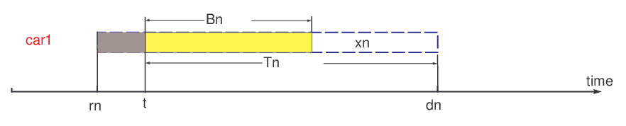
The state of the charging system consists of the state of individual chargers, charging cost, and ”period index”. The state of charger is defined by ; as illustrated in Fig. 2, is the lead time and is the remaining charging demand measured in charging time. If there is no EV attached to charger , we set .
The system charging cost is the cost of electricity. It is the electricity price from the wholesale market biased by the local renewable generation. Both of the wholesale price and the renewable generation are random and we assume the charging cost follows a Markov chain that is known to the scheduler.
We assume that the distribution of EV arrivals is time varying but periodic, i.e., the arrival distribution at the same period of each day is the same. Such a model allows us to incorporate a “typical day” travel pattern for arrival statistics and convert a non-stationary arrival to a cyclostationary one by introducing a “period index”. Specially, each day is equally divided into periods (for example, 24 hours) and the period state is the period index which forms a deterministic periodic Markov chain. The arrival rate and the probability mass function (PMF) of the initial state of EVs within the same period (for example, 9 AM-10 AM) across different days are assumed the same. The arrival rate and the initial state PMF within period , which are known to the scheduler, are denoted by and . Note that the Markov chain of charging costs needs not to be periodic (with length ).
Thus the state space of the charging system is defined by
.
Here, is the period space, the state space of the cost, and the state space of individual charger , for .
We note that the constructed MDP is stationary because the time dependency is incorporated by including in the system state a periodic Markov chain that describes time evolution.
II-A2 Action
The action of the scheduler is defined by where means that the charger is activated (active) whereas means that the charger is deactivated (passive).
II-A3 State evolution
We assume that the charging cost evolves as an exogenous finite state Markov chain with transition probability matrix . The evolution of the charging cost is independent of the actions taken by the scheduler.
The period state forms a deterministic periodic Markov chain. The evolution is stated as: where .
Given the period index , the evolution of chargers’ states depends on the scheduling action , i.e.,
EVs leave the chargers at their deadlines. New EVs arrive at the charging facility following a geometric distribution with probability . The probability mass function (PMF) governs the initial states of newly arrived EVs. The probability distribution of EV arrivals follows the periodic cycle with length , and depends only on period index (not ). Formally, the state evolution of charger with state under action is given by
| (1) |
where and is the maximum deadline and charging demand.
II-A4 Reward
At time , the reward received from charger under action is given by
| (2) |
where is an increasing and convex penalty function with . Note that the scheduler obtains one unit of reward if the EV is charged for one period. At the EV’s deadline, i.e., when , the scheduler pays the compensation for unfulfilled charging request, .
Given the initial system state and a policy that maps each system state to an action vector , the expected discounted system reward is defined by
| (3) |
where is the conditional expectation over the randomness in costs and EVs arrival under a given scheduling policy and is the discount factor. The analysis can be extended to the average case [41].
II-A5 Constrained MDP and optimal policy
We impose a constraint on the number of simultaneously activated chargers, i.e., for all . In practice, such a constraint limits the peak power consumption of the charging facility, due to feeder and transmission line capacity constraints.
The EV charging scheduling problem can be formulated as a constrained MDP. The maximum expected reward is given by
| (4) |
where is the action generated by policy . A policy is optimal if . Without loss of optimality, we will restrict our attention to stationary policies [42].
II-B A Performance Upper Bound
In (4), the power limit must be satisfied for all . By relaxing this constraint and requiring that the average power usage does not exceed , we obtain a performance upper bound for (4). In particular, a relaxed problem can be stated as
| (5) |
Problem (5) is not a practical formulation for the large scale EV charging since the power usage could be far more than at certain time.
Since the charging cost is the same for all chargers, the relaxed problem (5) is equivalent to the following problem (on the scheduling of a single charger ).
| (6) |
Problem (6) seeks to maximize the discounted reward from a single charger with no more than active action (per time period) on average. The optimal solution and the optimal objective of (6) are the same as those of (5). The optimal objective of (6) can be used as a performance upper bound for the original scheduling problem in (4).
III Whittle’s Index and Conservation law
Since the MDP formulation does not result in a scalable optimal scheduling policy, we seek to obtain an index policy [43] that can provide a scalable solution. An index policy schedules the charging of EVs based on the ranked order of indices associated with the states of chargers. Specifically, the index of charger is a mapping from its extended state to an index value. The index value of each state is independent from the states of other chargers and can be computed off-line which makes the index policy scalable.
III-A A Restless MAB Problem
We now formulate problem (4) as a restless multi-armed bandit (MAB) problem. The restlessness is due to the fact that the state of a charger, in particular, the lead time evolves even if the charger is not activated.
A complication of casting (4) as a restless MAB problem comes from the inequality constraint on the maximum number of simultaneous activated chargers. This complication can be circumvented by introducing dummy chargers and requiring that exactly chargers must be activated in each period. Specifically, each dummy charger always accrues zero reward, and the state of dummy chargers stays at . We let be the set of regular chargers and be the set of dummy chargers.
III-A1 Arms
The formulated restless multi-armed bandit (MAB) problem has arms: each arm represents a (regular or dummy) charger. We define the extended state of each charger as , and denote the extended state space as . The actions and the reward functions remain unchanged.
III-A2 MAB formulation
III-B The Whittle’s Index
We now examine the Whittle’s index policy for the restless MAB problem defined in (7). To this end, we first introduce the Whittle’s index and establish the indexability of the restless MAB problem in Theorem 1.
We consider the following single charger reward maximizing problem without constraint: given the initial state , policy activates and deactivates a single charger to maximize the reward without any power limit:
| (8) |
where is the value function of charger . Note that the value function defined above is different from the value function defined in (4) (for the constrained MDP).
Let be the Markov transition operator on the extended state and an arbitrary function defined as
The maximum discounted reward of problem (8) is determined by the Bellman equation
The Whittle’s index is defined by introducing a -subsidy problem, which is a modified version of the single charger problem defined in (8). In the -subsidy problem, whenever the passive action is taken, the scheduler receives an extra reward [12]. The Bellman equation for the single charger -subsidy problem is given by
| (9) |
where is the value function for the -subsidy problem.
Let denote the set of charger states under which it is optimal to take the passive action on charger in the -subsidy problem. Thus any state makes the first term in (9) larger or equal to the second term. We are now ready to define the indexability of an MAB problem.
Definition 1 (Indexability [12]).
Charger (arm) is indexable if the set increases monotonically from to as increases from to . The MAB problem is indexable if all the chargers (arms) are indexable.
Given the definition of indexability, the Whittle’s index is defined as follows.
Definition 2 (Whittle’s index [12]).
If charger (arm) is indexable, its Whittle’s index of the extended state is the infimum subsidy under which the passive action is optimal at state , i.e.,
If the charger is indexable, any will make the first term strictly smaller than the second term in (9) and it is optimal to activate the charger. Any will make the first term greater or equal to the second term and the optimal action is to deactivate the charger.
Given the definition of Whittle’s index, the Whittle’s index policy is stated as follows.
Definition 3 (Whittle’s index policy).
For a multi-charger (arm) problem defined in (7), the Whittle’s index policy sorts all chargers by the Whittle’s index value in a descend order and activates the first chargers.
III-C Indexability and Close-form Expression of Whittle’s Index
In this subsection, we show that the MAB problem is indexable and the Whittle’s index policy is optimal when the power limit is loose (). We also give the closed-form expression for the Whittle’s index when the charging cost is constant.
Theorem 1 (Indexability, optimality and closed-form indexes).
Proof.
An elementary proof of indexability can be found in Appendix -A. The proof of optimality of Whittle’s index policy with can be found in Appendix -B. The proof of closed-form of Whittle’s index with constant charging cost can be found in Appendix -C.
∎
In (10), when it is feasible to fulfill EV ’s charging request (i.e. its lead time is no less than its remaining processing time), EV ’s Whittle’s index is simply the (per-unit) charging profit . When non-completion penalty is inevitable, the index takes into account both the charging profit and the non-completion penalty. We note that the Whittle’s index gives higher priority to EVs with less laxity. Here, the laxity of charger is defined as (cf. Fig. 2).
When the power limit is loose (), the MAB problem breaks into independent single arm problems and Whittle’s index policy is optimal. It balances the charging cost and the penalty of non-finished demand by deactivating (regular) chargers when the charging cost is high. Simple index policies such as the earliest deadline first (EDF) and least laxity first (LLF) policies do not take charging cost into account and may lead to significant performance loss. However, when , we note that the Whittle’s index policy does not distinguish EVs with positive laxity, and is therefore suboptimal. In the next section we will introduce an enhanced heuristic policy based on the Whittle’s index.
IV Whittle’s Index Policy with LLLP Interchange
For the objective of time average () profit maximization, the Whittle’s index policy is shown (under some conditions on the evolution of arm states) to be asymptotically optimal, as the number of arms increases to infinity [44]. For the discounted profit maximization setting considered in this paper, the asymptotic optimality of Whittle’s index policy is not clear. For small systems with finitely many arms, there are counter-examples where an optimal index policy does not exist (and therefore the Whittle’s index policy cannot be optimal).
In this section, we will apply the Less Laxity and Longer remaining Processing time (LLLP) principle (originally proposed in [39]) to improve the Whittle’s index policy.
The LLLP principle is a priority rule for the scheduling of charging multiple EVs, which is defined as follows.
Definition 4 (The LLLP Principle).
Consider chargers (arms) and at time . We say dominates (), if has less laxity and longer remaining processing time, i.e., and , with at least one of the inequalities strictly holds.
LLLP defines a partial order over the EVs’ states such that the EV with less laxity and longer remaining charging demand should be given priority. In [39], the authors applied an interchange argument to show that LLLP could improve the performance of any given policy along every sample path, and further, there exists an optimal stationary policy that follows the LLLP principle under mild conditions.
To apply the LLLP principle, note that the Whittle’s index policy for the multi-armed bandit problem is a stationary policy: at each time it orders (the states of) the arms, and activates the first arms. The proposed heuristic policy re-order every pair of arms that violates the LLLP principle (cf. Algorithm 1). As such, the proposed heuristic policy always gives priority to EVs with less laxity and longer remaining processing time.
V Numerical Results
V-A Benchmark Policies
In this section, results of numerical experiments are presented to compare the performance of proposed index policy with other simple heuristic (index) policies, i.e., EDF (earliest deadline first) [13], LLF (least laxity first) [14], valley filling [30], and the original Whittle’s index (without LLLP interchange) [12].
If feasible, EDF charges EVs with the earliest deadlines, and LLF charges EVs with the least laxity. Both policies will fully utilize the capacity and charge EVs as long as there are at least unfinished EVs in the system. The Whittle’s index policy, on the other hand, ranks all chargers by the Whittle’s index and activates the first arms, and may put some (regular) chargers idle (deactivated) when the charging cost is high.
The centralized valley filling algorithm is proposed in [30] as an optimal offline scheduling policy for a setting with continuous charging rate, deterministic charging cost, and no newly arrival EVs. In our setting with newly incoming EVs, the algorithm is repeatedly executed based on the most updated information on the arrived EVs. At the beginning of each period, the algorithm schedules EV charging based on the information of all EVs that have arrived, assuming there is no new incoming EVs in the future. The charging schedule is carried out only for current time slot; at the beginning of the next period, the scheduling plan is recomputed. The (real-time adjusted version of) valley filling algorithm is used in our simulation as a benchmark.11 1 The original valley filling algorithm proposed in [30] has a hard constraint that all EVs’ charging request must be fulfilled. We note that it may not be feasible to fulfill all EVs’ charging requests under the charging capacity . When implementing the valley filling algorithm in our setting, we modify the objective function of the valley filling algorithm so as to maximize the total reward subject to the maximum power limit; in its objective function, the charging reward is calculated based on expected future charging cost and the non-completion penalty function (introduced in (2)).
V-B Numerical Results
We first considered a special case of problem (7) with a constant charging cost. Since the charging cost was time-invariant, it was optimal to fully utilize the charging capacity to charge unfinished EVs.
In Fig. 3, we fixed the traffic of EVs and the total number of regular chargers and varied the power limit . All policies besides the EDF scheduling performed well and close to the upper bound of the performance. When , all EVs can be fully charged. Thus all policies achieved optimality. In Fig. 4, we zoomed in the case when and varied the total number of regular charger . We observed that the Whittle’s index policy with LLLP interchange and LLF achieved similar performance, since both policies roughly followed the least laxity first principle. The performance of these two policies was close to the performance upper bound. The EDF policy performed poorly because it did not take the remaining charging demand into account. The gap between the Whittle’s index policy and the Whittle’s index policy with LLLP interchange came from the reordering of EVs with positive laxity (cf. the discussion following Theorem 1).


For the dynamic charging cost case, we used the real-time pricing signal from the California Independent System Operator (CAISO) and trained a Markovian model that describes the marginal charging costs (cf. Sections III and V of [40]). Each period of the constructed Markov chain (on charging cost) lasted for 1 hour, and each periodic cycle lasted for one day with . For each period, the real-time price was quantized into discrete price states, and the transition probability (of the Markov chain) was simply the frequency the price changed from one state to another.

In Fig. 5, we fixed the EV traffic and the total number of regular chargers and varied the power limit constraints. When the power limit was low and is small, there was no enough power to charge EVs and the penalty dominated the charging profit. In this case the performance of different policies were close since the limited resource allowed not much to do. When the power limit was adequate and , all EVs could be fully charged on time. In this case, the Whittle’s index policy solved the problem optimally as stated in Theorem 1 and achieved the upper bound. The interchange did not happen because the LLLP principle was always satisfied in this case. The valley filling algorithm did not consider the future arrivals and EDF and LLF did not consider the dynamic charging cost, thus they performed sub-optimal. When the power constraint was neither too tight () nor too loose (), LLLP could reduce the number of unfinished EVs with large remaining charging demand and therefore reduced the non-completion penalties.

In Fig. 6, we compared the performance of different policies by fixing the power limit ratio and varied the number of regular chargers. Both EDF and LLF sought to activate as many regular chargers as possible, up to the capacity constraint . The Whittle’s index policy, on the other hand, took the advantage of the pricing fluctuation and charged more EVs at price valley and kept some chargers idle when charging cost was high. Based on the Whittle’s index policy, the LLLP interchange reduced the penalty of unfinished EVs and improved the performance of Whittle’s index policy. The total reward achieved by the Whittle’s index with LLLP interchange policy was more than 1.7 times of that obtained by EDF; the performance gap between the the Whittle’s index with LLLP interchange policy and the LLF policy was over . We also noted that the LLLP principle improved Whittle’s index by around .
VI Conclusion
We considered the problem of scheduling of large scale EV charging in public facilities—a problem of particular potential significance as EV penetration deepens. In such settings, it is essential to develop highly efficient and online charging algorithms. To this end, index policies considered in this paper are attractive for its implementation simplicity and versatility in incorporating various operation uncertainties.
-A Proof of Indexability
In this subsection, we provide an elementary proof of indexability. That is, for any charger state , there is a critical such that if and only if the first term in the Bellman equation (9) is larger or equal to the the second term in a single charger -subsidy problem.
The indexability of dummy chargers is straightforward. For , there is no EV arrival, and only the charging cost and period index evolve. The Bellman equation of the -subsidy problem is given by
If and only if , the first term is larger than the second term and it is optimal to deactivate the dummy charger. Otherwise, the active action is optimal. So a dummy charger is indexable and its Whittle’s index is .
For the regular chargers, we prove the indexability by induction.
-A1 When
There is no EV attached to the charger. The Bellman equation is stated as
where
is the expected reward of possible arrivals. If and only if , the first term is larger and the passive action is optimal. Thus .
-A2 When
There are two possible conditions.
- •
If , the Bellman equation is stated as
Thus .
- •
If , the Bellman equation is stated as
If and only if , the passive action is optimal.
Thus the arm is indexable and the Whittle’s index for is stated as follows.
We summarize some properties of the Whittle’s index prove them for the case .
Proposition 1 (Monotonicity of Whittle’s index).
Whittle’s index is non-decreasing in the charging demand when .
Proof.
Since the penalty function is convex, Whittle’s index is nondecreasing when and . ∎
Proposition 2 (Difference of value functions).
Denote the difference of the value function as
where and is the maximum charging demand.
Thus is piecewise linear in and has following properties.
- •
is continuous in .
- •
There exist and such that, is piecewise linear and when . Otherwise, is constant .
Proof.
- •
When ,
If ,
If ,
- •
When ,
Since ,
Thus, is piecewise linear and continuous in . The derivative satisfies Property 2. ∎
Proposition 3 (Concavity of value functions).
The difference of value functions is non-increasing in when . Thus is concave in when .
Proof.
Since when , is nondecreasing in ,
The first and last cases are non-positive since the penalty function is convex. The second and third cases are non-positive because of the expressions of the index . Thus is concave in when . ∎
-A3
If , the Bellman equation is stated as follows.
If and only if , the first term is larger than the second term and the passive action is optimal. Thus .
If , the Bellman equation is stated as follows.
| (11) |
Denote the difference between the two actions as
where
So is continuous and non-decreasing in . When , . When , . Thus there is a cross point of and the x-axis. Define . If and only if , the first term in (11) is larger or equal to the second term and the passive action is optimal. By definition, is the Whittle’s index.
The indexability of is shown. Next we will prove Proposition 1, 2, 3 for assuming that they are true for .
Proof of Proposition 2.
If ,
- •
If ,
- •
If ,
If ,
- •
If ,
- •
If ,
Denote
and
where
Since Proposition 2 holds for by assumption, we have is continuous in . When , is piece-wise linear and . Otherwise, is constant. ∎
Proof of Proposition 3.
Since is nondecreasing in when ,
The first and forth cases are non-positive because is concave when according to the assumption. The second and third cases are non-positive because of the expressions of . Thus is concave in when . ∎
-B Proof of Optimality of Whittle’s Index with
In this appendix, we prove that the Whittle’s index policy optimally solves the MAB problem defined in (7), which is equivalent to the MDP problem formulated in (4).
First, we claim that the Whittle’s index policy optimally solves the single charger problem with dynamic price and no constraint, as defined in (8). The extended state includes the charging cost and period index. The Bellman equation of the single charger problem is given by:
| (12) |
where action means to activate the charger and means to leave it passive.
The Whittle’s index is defined by introducing a -subsidy problem, which is a modified version of the single arm problem defined in (12). In the -subsidy problem, whenever the passive action is taken, the scheduler receives an extra reward [12]. The single charger problem defined in (12) is simply the case when the subsidy .
The Bellman equation for the -subsidy problem is given by
| (13) |
where is the value function for the -subsidy problem.
Now define a Whittle’s index policy for a single charger (either regular or dummy charger) -subsidy problem as to activates the charger if and only if . Thus we have the following lemma.
Lemma 1.
Proof.
We have shown in Appendix -A that the Whittle’s index defined in Definition 2 exists, and therefore the Whittle’s index policy is well defined. By Definition 2, for any state such that , the first term in (13) is strictly smaller than the second term. The Whittle’s index policy activates the charger and obtains the second term as an expected reward which satisfies the Bellman equation in this case.
For , the first term is greater or equal to the second term in the Bellman equation by Definition 2. The indexability result proved in Appendix -A guarantees that the passive set grows monotonously which implies that this inequality is true for any . Thus, for any state such that , the Whittle’s index policy leaves the charger passive and obtains the first term as the expected reward, satisfying the Bellman equation.
Now we consider the problem (7) with : we have a regular charger and a dummy charger, and at each time, we are required to activate exact one charger. For this constrained two-arm problem, the state is defined as , where is the extended state of the regular charger and the state of the dummy charger. The action means to activate the regular charger, and represents activating the dummy charger.
The state of the dummy charger will always be 0. The dummy charger yields no reward regardless of the taken action. Thus the state transition of two-arm problem is equivalent to the state transition in problem (12), i.e., . The rewards of the two-arm problem can be presented by the rewards of the single charger problem in (12):
The Whittle’s index policy for the two-arm problem (denoted by ) activates the regular charger when , and activates the dummy charger (leaving the regular charger passive) otherwise.
When faces state and faces state for the same realization , the actions of two policies are the same. will activate the regular charger in the two-arm problem if and only if activates the charger in the single charger problem, and vice versa. Since the reward, transition and the action of these two policies are the same, the value functions will be the same. Denoting the value function of and by and , we have . Since satisfies the Bellman equation (12), we have
which is in fact the Bellman equation for the constrained two-arm problem. The Whittle’s index policy satisfies the Bellman equation for the two-arm problem and is therefore optimal.
Finally, we argue that the Whittle’s index policy is optimal for the multi-arm problem defined in (7). We have regular chargers and dummy chargers. At each time, we activate exact chargers. We can pair each regular charger with¡¡a dummy charger and implement the Whittle’s index policy for each pair. The action of each regular charger is decoupled, and the total reward is simply the sum of reward from all the regular chargers. The Whittle’s index policy optimally optimal solves the problem of each pair, and is therefore optimal for the original problem in (7). We note, however, that the above argument no longer holds when , because the problem defined in (7) cannot be decoupled into single (regular) charger problems in this case.
-C Proof of Closed-form of Whittle’s Index
Proof.
Since the cost is constant, we will omit the cost in the state of chargers for simplicity.
For dummy chargers, there is no EV arrival, and only the charging cost evolves. The Bellman equation of the -subsidy problem is given by
When , it is optimal to activate the dummy charger. Otherwise, passive action is optimal. So a dummy charger is indexable and its Whittle’s index is .
For regular chargers, we showed in Appendix B2 that and when . We will show the index closed-form for the case of using induction.
-C1 When
The discussion is divided into following two conditions.
If ,
The difference between active and passive actions
equals to when . Thus .
If , the Bellman equation is stated as follows.
Denote . The difference between active and passive actions
equals to when . Thus .
-C2 When
Assume Equation (10) holds for , consider the case for .
If ,
The difference between actions is
The last case can be rewritten as
which equals to when since by assumption. Thus .
If , the difference between actions is stated as follows.
The latter case equals to when since when by assumption. Thus when .
If ,
equals to when . So when .
So when , the first case in equation (14) equals to . Thus when , the closed-form of index is stated as:
∎
References
- [1] F. Creutzig, P. Jochem, O. Y. Edelenbosch, L. Mattauch, D. P. van Vuuren, D. McCollum, and J. Minx, “Transport: A roadblock to climate change mitigation?” Science, vol. 350, no. 6263, pp. 911–912, 2015.
- [2] Electric Drive Transportation Association, “Electric drive sales dashboard,” 2015, accessed in May 2015 from: http://electricdrive.org/index.php?ht=d/sp/i/20952/pid/20952.
- [3] International Energy Agency, “Global EV outlook 2015,” 2015, accessed in May 2015 from: http://www.iea.org/evi/Global-EV-Outlook-2015-Update_1page.pdf.
- [4] U.S. Department of Energy, “Electric vechicle charging station locations,” 2015, accessed in May 2015 from: http://www.afdc.energy.gov/fuels/electricity_locations.html.
- [5] Z. Yu, S. Li, and L. Tong, “On market dynamics of electric vehicle diffusion,” in Proceedings of the 52nd Annual Allerton Conferene on Communication, Control, and Computing, Oct. 2014.
- [6] J. Winebrake and A. Farrell, “The AFV program and its role in future AFV market development,” Transportation Rewsearch Part D, vol. 2, no. 2, pp. 125–132, 1997.
- [7] W. Kempton and J. Tomić, “Vehicle-to-grid power implementation: From stabilizing the grid to supporting large-scale renewable energy,” Journal of Power Sources, vol. 144, no. 1, pp. 280–294, 2005.
- [8] A. N. Brooks, Vehicle-to-grid demonstration project: Grid regulation ancillary service with a battery electric vehicle. California Environmental Protection Agency, Air Resources Board, Research Division, 2002.
- [9] K. Clement-Nyns, E. Haesen, and J. Driesen, “The impact of charging plug-in hybrid electric vehicles on a residential distribution grid,” IEEE Transactions on Power Systems, vol. 25, no. 1, pp. 371–380, 2010.
- [10] E. Sortomme, M. M. Hindi, S. J. MacPherson, and S. Venkata, “Coordinated charging of plug-in hybrid electric vehicles to minimize distribution system losses,” IEEE Transactions on Smart Grid, vol. 2, no. 1, pp. 198–205, 2011.
- [11] Z. Yu, Y. Xu, and L. Tong, “Large scale charging of electric vehicles: A multi-armed bandit approach,” in 2015 53rd Annual Allerton Conference on Communication, Control, and Computing (Allerton). IEEE, 2015, pp. 389–395.
- [12] P. Whittle, “Restless bandits: Activity allocation in a changing world,” Journal of applied probability, pp. 287–298, 1988.
- [13] C. L. Liu and J. W. Layland, “Scheduling algorithms for multiprogramming in a hard-real-time environment,” Journal of ACM, vol. 20, pp. 46–61, 1973.
- [14] M. Dertouzos, “Control robotics: the procedural control of physical processes,” in Proceedings of International Federation for Information Processing Congress, 1974, pp. 807–813.
- [15] S. S. Panwar, D. Towsley, and J. K. Wolf, “Optimal Scheduling Policies for a class of Queues with Customer Deadlines to the Beginning of Service,” Journal of Association for Computing Machinery, vol. 35, no. 4, pp. 832–844, October.
- [16] D. Towsley and S. Panwar, “On the Optimality of Minimum Laxity and Earliest Deadline Scheduling for Real-Time Multiprocessors,” in Proceedings of IEEE Euromicro 90’ Workshop on Real-Time, Jun. 1990, pp. 17–24.
- [17] R. I. Davis and A. Burns, “A survey of hard real-time scheduling for multiprocessor systems,” ACM Computing Surveys, vol. 43, no. 4, 2011.
- [18] M. L. Dertouzos and A. K. Mok, “Multiprocessor online scheduling of hard-real-time tasks,” IEEE Transactions on Software Engineering, vol. 5, pp. 1497–1506, 1989.
- [19] P. P. Bhattacharya and A. Ephremides, “Optimal scheduling with strict deadlines,” IEEE Transactions on Automatic Control, vol. 34, no. 7, pp. 721–728, 1989.
- [20] P. P. Bhattacharya, L. Tassiulas, and A. Ephremides, “Optimal scheduling with deadline constraints in tree networks,” IEEE Transactions on Automatic Control, vol. 42, no. 12, pp. 1703–1705, 1997.
- [21] V. Raghunathan, V. Borkar, M. Cao, and P. R. Kumar, “Index policies for real-time multicast scheduling for wireless broadcast systems,” in INFOCOM 2008. The 27th Conference on Computer Communications. IEEE. IEEE, 2008.
- [22] J. J. Jaramillo, R. Srikant, and L. Ying, “Scheduling for optimal rate allocation in ad hoc networks with heterogeneous delay constraints,” IEEE Journal on Selected Areas in Communications, vol. 29, no. 5, pp. 979–987, 2011.
- [23] Z. Yu, S. Chen, and L. Tong, “An intelligent energy management system for large-scale charging of electric vehicles,” CSEE Journal of Power and Energy Systems, vol. 2, no. 1, pp. 47–53, 2016.
- [24] S. Chen, L. Tong, and T. He, “Optimal deadline scheduling with commitment,” in Proceedings of 2011 49th Annual Allerton Conference on Communication, Control, and Computing. IEEE, 2011, pp. 111–118.
- [25] S. Chen, Y. Ji, and L. Tong, “Large scale charging of electric vehicles,” in Proceedings of 2012 IEEE Power and Energy Society General Meeting. IEEE, 2012, pp. 1–9.
- [26] S. Chen and L. Tong, “iEMS for large scale charging of electric vehicles: Architecture and optimal online scheduling,” in Proceedings of 2012 IEEE Third International Conference on Smart Grid Communications. IEEE, 2012, pp. 629–634.
- [27] A. Subramanian, M. Garcia, A. Dominguez-Garcia, D. Callaway, K. Poolla, P. Varaiya et al., “Real-time scheduling of deferrable electric loads,” in American Control Conference (ACC), 2012. IEEE, 2012, pp. 3643–3650.
- [28] Z. Ma, D. S. Callaway, and I. Hiskens, “Decentralized charging control for large populations of plug-in vehicles,” IEEE Transactions on Control System Technology, vol. 28, no. 1, pp. 67–78, 2013.
- [29] E. L. Karfopoulos and N. D. Hatziargyriou, “A multi-agent system for controlled charging of a large population of electric vehicles,” IEEE Transactions on Power Systems, vol. 28, no. 2, pp. 1196–1204, 2013.
- [30] L. Gan, U. Topcu, and S. Low, “Optimal decentralized protocols for electric vehicle charging,” IEEE Transactions on Power Systems, vol. 28, no. 2, pp. 940–951, 2013.
- [31] G. Benetti, M. Delfanti, T. Facchinetti, D. Falabretti, and M. Merlo, “Real-time modeling and control of electric vehicles charging processes,” IEEE Transactions on Smart Grid, vol. 6, no. 3, pp. 1375–1385, 2015.
- [32] S. Deilami, A. S. Masoum, P. S. Moses, and M. A. Masoum, “Real-time coordination of plug-in electric vehicle charging in smart grids to minimize power losses and improve voltage profile,” IEEE Transactions on Smart Grid, vol. 2, no. 3, pp. 456–467, 2011.
- [33] X. Luo and K. W. Chan, “Real-time scheduling of electric vehicles charging in low-voltage residential distribution systems to minimise power losses and improve voltage profile,” Generation, Transmission & Distribution, IET, vol. 8, no. 3, pp. 516–529, 2014.
- [34] C. Wu, H. Mohsenian-Rad, and J. Huang, “Vehicle-to-aggregator interaction game,” IEEE Transactions on Smart Grid, vol. 3, no. 1, pp. 434–442, 2012.
- [35] J. Donadee and M. D. Ilić, “Stochastic optimization of grid to vehicle frequency regulation capacity bids,” IEEE Transactions on Smart Grid, vol. 5, no. 2, pp. 1061–1069, 2014.
- [36] S. Vagropoulos, A. G. Bakirtzis et al., “Optimal bidding strategy for electric vehicle aggregators in electricity markets,” IEEE Transactions on Power Systems, vol. 28, no. 4, pp. 4031–4041, 2013.
- [37] E. Sortomme and M. A. El-Sharkawi, “Optimal scheduling of vehicle-to-grid energy and ancillary services,” IEEE Transactions on Smart Grid, vol. 3, no. 1, pp. 351–359, 2012.
- [38] F. Juul, M. Negrete-Pincetic, J. MacDonald, and D. Callaway, “Real-time Scheduling of Electric Vehicles for Ancillary Services,” in Proceedings of 2015 IEEE Power and Energy Society General Meeting, Denver, CO, 2015.
- [39] Y. Xu and F. Pan, “Scheduling for charging plug-in hybrid electric vehicles,” in Proceedings of 2012 IEEE 51st Annual Conference on Decision and Control (CDC). IEEE, 2012, pp. 2495–2501.
- [40] S. Kwon, Y. Xu, and N. Gautam, “Meeting inelastic demand in systems with storage and renewable sources,” IEEE Tranactions on Smart Grid.
- [41] P. K. Dutta, “What do discounted optima converge to?: A theory of discount rate asymptotics in economic models,” Journal of Economic Theory, vol. 55, no. 1, pp. 64–94, 1991.
- [42] E. Altman, Constrained Markov decision processes. CRC Press, 1999, vol. 7.
- [43] J. C. Gittins, “Bandit Processes and Dynamic Allocation Indices,” Journal of the Royal Statistical Society, vol. 41, no. 2, pp. 148–177, 1979.
- [44] J. Nino-Mora et al., “Restless bandits, partial conservation laws and indexability,” Advances in Applied Probability, vol. 33, no. 1, pp. 76–98, 2001.