跳到论文正文
W Papers独立论文阅读器 arXiv:1605.07279 论文正文 计算阅读时间 · 0%
引用这篇论文根据当前论文元数据生成,正式投稿前建议核对。


License: arXiv.org perpetual non-exclusive license
arXiv:1605.07279v1 [math.AP] 24 May 2016

Evolution of Interfaces for the Nonlinear Parabolic p-Laplacian Type Reaction-Diffusion Equations

Ugur G. Abdulla and Roqia Jeli

Department of Mathematics, Florida Institute of Technology, Melbourne, Florida 32901

Abstract. We present a full classification of the short-time behaviour of the interfaces and local solutions to the nonlinear parabolic pp-Laplacian type reaction-diffusion equation of non-Newtonian elastic filtration

ut−(|ux|p−2​ux)x+b​uβ=0,p>2,β>0u_{t}-\Big(|u_{x}|^{p-2}u_{x}\Big)_{x}+bu^{\beta}=0,\ p>2,\beta>0

The interface may expand, shrink, or remain stationary as a result of the competition of the diffusion and reaction terms near the interface, expressed in terms of the parameters p,β,s​i​g​n​bp,\beta,sign~b, and asymptotics of the initial function near its support. In all cases, we prove the explicit formula for the interface and the local solution with accuracy up to constant coefficients. The methods of the proof are based on nonlinear scaling laws, and a barrier technique using special comparison theorems in irregular domains with characteristic boundary curves.

1 Inrtroduction

We consider the Cauchy problem(CP) for the nonlinear degenerate parabolic equation

(1.1) L​u≡ut−(|ux|p−2​ux)x+b​uβ=0,x∈ℝ,0<t<T,Lu\equiv u_{t}-\Big(|u_{x}|^{p-2}u_{x}\Big)_{x}+bu^{\beta}=0,\ x\in\mathbb{R},0<t<T,

with

(1.2) u⁡(x,0)=u0​(x),x∈ℝ,u(x,0)=u_{0}(x),~~x\in\mathbb{R},

where  p>2,b∈ℝ,β>0,0<T≤+∞,p>2,~b\in\mathbb{R},~\beta>0,~0<T\leq+\infty,  and u0u_{0} is nonnegative and continuous. We assume that  b>0b>0 if β<1\beta<1, and bb is arbitrary if  β≥1\beta\geq 1 (see Remark 1.1). Equation (1.1) arises in many applications, such as the filtration of non-Newtonian fluids in porous media ([8] or nonlinear heat conduction ([9]) in the presence of the reaction term expressing additional release (b>0b>0) or absorption (b<0b<0) of energy.

The goal of this paper is to analyze the behavior of interfaces separating the regions where  u=0u=0 and where  u>0u>0. We present full classification of the short-time evolution of interfaces and local structure of solutions near the interface. Due to invariance of (1.1) with respect to translation, without loss of generality, we will investigate the case when  η⁡(0)=0,\eta(0)=0, where

η⁡(t)=sup​{x:u⁡(x,t)>0}.\eta(t)=\text{sup}~\{x:u(x,t)>0\}.

and precisely, we are interested in the short-time behavior of the interface function  η⁡(t)\eta(t) and local solution near the interface. We shall assume that

(1.3) u0∼C​(−x)+α​as​x→0−for some​C>0,α>0.u_{0}\sim C(-x)_{+}^{\alpha}~~\text{as}~x\rightarrow 0-~~~\text{for some}~~~C>0,~\alpha>0.

The direction of the movement of the interface and its asymptotics is an outcome of the competition between the diffusion and reaction terms and depends on the parameters  p,b,β,C,p,b,\beta,C, and α\alpha. Since the main results are local in nature, without loss of generality we may suppose that  u0u_{0} either is bounded or satisfies some restriction on its growth rate as  x→−∞x\rightarrow-\infty which is suitable for existence, uniqueness, and comparison results (see section 3). The special global case

(1.4) u0​(x)=C​(−x)+α,x∈ℝ,u_{0}(x)=C(-x)_{+}^{\alpha},\quad x\in\mathbb{R},

will be considered when the solution to the problem (1.1), (1.4) is of self-similar form. Our estimations are global in time in these special cases.

Initial development of interfaces and structure of local solution near the interfaces is very well understood in the case of the reaction-diffusion equations with porous medium type diffusion term:

(1.5) ut−(um)x​x+b​uβ=0​x∈ℝ,0<t<T,u_{t}-(u^{m})_{xx}+bu^{\beta}=0\ x\in\mathbb{R},0<t<T,

Full classification of the evolution of interfaces and the local behaviour of solutions near the interfaces in CP (1.5), (1.2), (1.3) was presented in [1] for the case of fast diffusion (m>1m>1) case, and in [2] for the slow diffusion (0<m<10<m<1) case. The major obstacle in solving the interface development problem for nonlinear degenerate parabolic equations is a problem of non-uniform asymptotics in the sense of singular perturbations theory, namely that the dominant balance as  t→0+t\rightarrow 0+ between the terms in (1.1), (1.5) on curves which approach the boundary of the support on the initial line depending on how they do so. The general theory, including existence, boundary regularity, uniqueness and comparison theorems, for the reaction diffusion equations of type (1.5) in general non-cylindrical and non-smooth domains is developed in [3] in the one-dimensional case, and in [5, 6, 7] in the multi-dimensional case. Comparison theorems proved in [3] were essential tools in developing the rigorous proof method in [1, 2] for solving interface problem for the reaction-diffusion equation (1.5). The rigorous proof method developed in [1, 2] is based on a barrier technique using special comparison theorems in irregular domains with characteristic boundary curves. In this paper we apply the method developed in [1] to solve the interface problem for the PDE (1.1).

The structure of the paper is as follows: In section 2 we outline the main results. In section 3 we apply rescaling and prove for some preliminary estimations which are necessary for using our barrier technique. Finally in section 4 we prove the results of section 2. To avoid technical difficulties, we give explicit values of some of lengthy constants in the appendix.

Remark 1.1. We are not interested in the special case p=2p=2 of semilinear heat equation. This case was completed in [15, 16] (see also [1]). However, we will mention when our results extend to the limit case p=2p=2. In general, the case p=2p=2 is in some sense a singular limit. For example, if b>0,0<β<1,α<pp−1−βb>0,0<\beta<1,\alpha<\frac{p}{p-1-\beta}, then we prove that the interface initially expands and

η⁡(t)∼C1​t1/(p−α⁡(p−2))​as​t→0+.\eta(t)\sim C_{1}t^{1/(p-\alpha(p-2))}~~\text{as}~t\rightarrow 0+.

By passing to the limit as p↓2p\downarrow 2 formally, this yields a false result. In fact, from [16] it follows that if  p=2p=2, then

η⁡(t)∼C2​(t​log⁡1t)12as​t→0+\eta(t)\sim C_{2}\Big(t\log\frac{1}{t}\Big)^{\frac{1}{2}}\quad\text{as}~t\rightarrow 0+

2 Description of main results.

Refer to caption
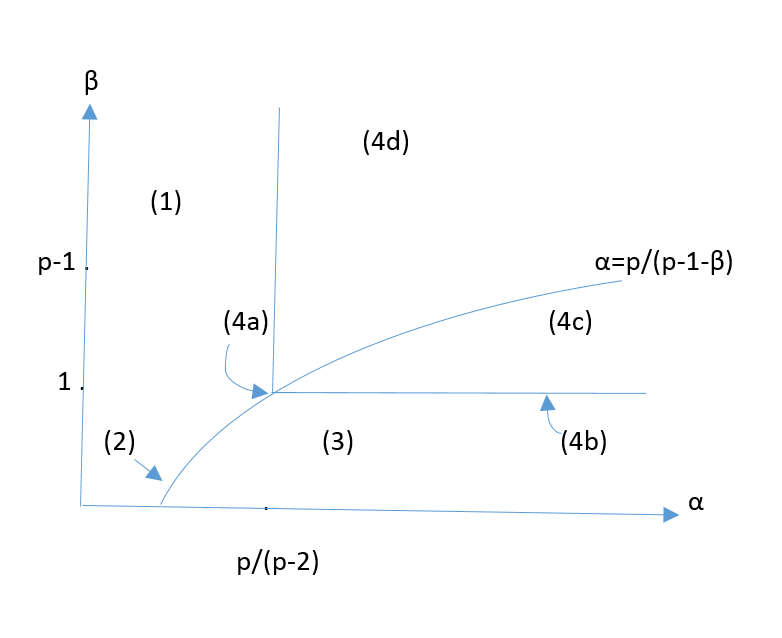
Figure 1: Classification of different cases in the (α\alpha,β\beta) plane for interface development in problem (1.1)-(1.4).

In Figure 1 we present classification diagram in (α,β)(\alpha,\beta)-plane for the initial interface development in CP (1.1), (1.2), (1.3) if b>0b>0.

  • •

    Region (1): α<p/(p−1−min⁡{1,β});\alpha<p/(p-1-\min\{1,\beta\}); Diffusion dominates and interface expands.

  • •

    Region (2): α=p/(p−1−β),0<β<1;\alpha=p/(p-1-\beta),0<\beta<1; Diffusion and absorption are in balance in this borderline case. There is a critical constant C∗C_{*} such that interface expands for C>C∗C>C_{*}, and shrinks for C<C∗C<C_{*}.

  • •

    Region (3): α>p/(p−1−β),0<β<1;\alpha>p/(p-1-\beta),0<\beta<1; Absorption term dominates and interface shrinks.

  • •

    Region (4): α≥p/(p−2),β≥1;\alpha\geq p/(p-2),\beta\geq 1; Interface has initial ”waiting time”.

To describe the asymptotic properties of the interface and local solution near the interface, we divide the results into the two different subcases:
(I)  b≠0(eitherb>0,β>0orb<0,β≥1)b\neq 0\ (\text{either}~b>0,\beta>0\ \text{or}~b<0,\beta\geq 1) and  p>2;p>2; (II)  b=0b=0.

(I) In this case there are four different subcases, as shown in Figure 1 and itemized above. (In view of our assumptions, the case b<0b<0 relates to the part of the (α,β\alpha,\beta) plane with  β≥1.)\beta\geq 1.)

Region (1): Let  α<pp−1−min​{1,β}.\alpha<\frac{p}{p-1-\text{min}\{1,\beta\}}. In this case the interface initially expands and

(2.1) η⁡(t)∼ξ∗​t1/(p−α⁡(p−2))​as​t→0+,\eta(t)\sim\xi_{*}t^{1/(p-\alpha(p-2))}~~\text{as}~t\rightarrow 0+,

where

(2.2) ξ∗=Cp−2p−α⁡(p−2)​ξ∗′\xi_{*}=C^{\frac{p-2}{p-\alpha(p-2)}}\xi^{\prime}_{*}

and  ξ∗′>0\xi^{\prime}_{*}>0 depends on pp  and  α\alpha only (see Lemma 2). For ∀\forall ρ<ξ∗\rho<\xi_{*} ∃\exists f⁡(ρ)>0f(\rho)>0 depending on  C,p,C,p, and α\alpha  such that

(2.3) u⁡(x,t)∼f⁡(ρ)​t(α/p−α⁡(p−2))a​st→0+u(x,t)\sim f(\rho)t^{(\alpha/p-\alpha(p-2))}~~~~as~~~~t\rightarrow 0+

along the curve  x=ξρ​(t)=ρ​t1/(p−α⁡(p−2)).x=\xi_{\rho}(t)=\rho t^{1/(p-\alpha(p-2))}. A function ff is a shape function of the self-similar solution of (1.1),(1.4) with b=0b=0 (see Lemma 2):

(2.4) u∗​(x,t)=tαp−α⁡(p−2)​f​(ξ),ξ=x​t−1p−α⁡(p−2),u_{*}(x,t)=t^{\frac{\alpha}{p-\alpha(p-2)}}f(\xi),\quad~~~\xi=xt^{-\frac{1}{p-\alpha(p-2)}},

In fact, ff is a unique solution of the following nonlinear ODE problem:

(2.5) {(|f′​(ξ)|p−2​f′​(ξ))′+1p−α⁡(p−2)​ξ​f′​(ξ)−αp−α⁡(p−2)​f​(ξ)=0,−∞<ξ<ξ∗f⁡(−∞)∼C​(−ξ)α,f⁡(ξ∗)=0,f⁡(ξ)≡0,ξ≥ξ∗\begin{cases}\big(|f^{\prime}(\xi)|^{p-2}f^{\prime}(\xi)\big)^{\prime}+\frac{1}{p-\alpha(p-2)}\xi f^{\prime}(\xi)-\frac{\alpha}{p-\alpha(p-2)}f(\xi)=0,~-\infty<\xi<\xi_{*}\\ f(-\infty)\sim C(-\xi)^{\alpha},f(\xi_{*})=0,f(\xi)\equiv 0,~\xi\geq\xi_{*}\end{cases}

Its dependence on CC is given through the following relation:

(2.6a) f⁡(ρ)=Cp/(p−α⁡(p−2))​f0​(C(p−2)/(α⁡(p−2)−p)​ρ),f(\rho)=C^{p/(p-\alpha(p-2))}f_{0}\Big(C^{(p-2)/(\alpha(p-2)-p)}\rho\Big),
(2.6b) f0​(ρ)=w⁡(ρ,1),ξ∗′=sup​{ρ:f0​(ρ)>0}>0f_{0}(\rho)=w(\rho,1),~~~\quad\xi^{\prime}_{*}=\text{sup}\{\rho:f_{0}(\rho)>0\}>0

where  ww is a solution of (1.1), (1.4) with  b=0,C=1.b=0,C=1. Lower and upper estimations for  ff are given in (2.28). Moreover,

(2.7) ξ∗′=A0p−2p​[(p−1)p−1​(p−α⁡(p−2))(p−2)p−1]1p​ξ∗′′,\xi^{\prime}_{*}=A_{0}^{\frac{p-2}{p}}\Big[\frac{(p-1)^{p-1}(p-\alpha(p-2))}{(p-2)^{p-1}}\Big]^{\frac{1}{p}}\xi^{\prime\prime}_{*},

where  A0=w⁡(0,1)A_{0}=w(0,1) and  ξ∗′′\xi^{\prime\prime}_{*} is some number in  [ξ1,ξ2],[\xi_{1},\xi_{2}], where

ξ1=(p−1)1p​(α⁡(p−2))−1p,ξ2=1if​(p−1)​(p−2)−1≤α<p​(p−2)−1,\xi_{1}=(p-1)^{\frac{1}{p}}\Big(\alpha(p-2)\Big)^{-\frac{1}{p}},~~~~\xi_{2}=1\quad~~~~~~~~~~~~~\text{if}~~~(p-1)(p-2)^{-1}\leq\alpha<p(p-2)^{-1},
(2.8) ξ1=1,ξ2=(p−1)1p​(α⁡(p−2))−1p,if​0<α≤(p−1)​(p−2)−1.\xi_{1}=1,~~~~~~~~~~~~~~~~~\xi_{2}=(p-1)^{\frac{1}{p}}\Big(\alpha(p-2)\Big)^{-\frac{1}{p}},~~~~~~~~~~~~\text{if}~~~0<\alpha\leq(p-1)(p-2)^{-1}.

In particular, if  α=(p−1)​(p−2)−1\alpha=(p-1)(p-2)^{-1}and p>1+(min​{1,β})−1p>1+(\text{min}\{1,\beta\})^{-1}, then the explicit solution of the problem (1.1), (1.4) with b=0b=0 is given by (2.24) and we have

(2.9) ξ1=ξ2,ξ∗′=(p−1)p−1​(p−2)1−p,f0​(x)=(ξ∗′−x)+(p−1)/(p−2)\xi_{1}=\xi_{2},~~~\xi^{\prime}_{*}=(p-1)^{p-1}(p-2)^{1-p},~~~~f_{0}(x)=\big(\xi^{\prime}_{*}-x\big)_{+}^{(p-1)/(p-2)}

The explicit formulae (2.1) and (2.3) mean that the local behavior of the interface and solution along  x=ξρ​(t)x=\xi_{\rho}(t) coincide with those of the problem (1.1), (1.4) with  b=0b=0.

Region (2): Let  b>0,0<β<1,α=p/(p−1−β)b>0,0<\beta<1,\alpha=p/(p-1-\beta) (here we describe the results for the case p=2 as well ). In this borderline case the direction of the movement of the interface depends on the constant CC. The critical value is

C∗=[|b|​(p−1−β)p(1+β)​pp−1​(p−1)]1p−1−βC_{*}=\Big[\frac{|b|(p-1-\beta)^{p}}{(1+\beta)p^{p-1}(p-1)}\Big]^{\frac{1}{p-1-\beta}}

First, assume that u0u_{0} is defined by (1.4). If  β⁡(p−1)=1\beta(p-1)=1, then the explicit solution to (1.1), (1.4) is

(2.10) u⁡(x,t)=C​(ζ∗​t−x)+11−β,ζ∗=b⁡(1−β)​Cβ−1​((C/C∗)p−1−β−1).u(x,t)=C(\zeta_{*}t-x)_{+}^{\frac{1}{1-\beta}},~~~~~\zeta_{*}=b(1-\beta)C^{\beta-1}((C/C_{*})^{p-1-\beta}-1).

It has an expanding interface if  C>C∗C>C_{*} , a shrinking interface if 0<C<C∗0<C<C_{*} , and is a stationary solution if C=C∗C=C_{*}.

Let β⁡(p−1)≠1.\beta(p-1)\neq 1. If C=C∗C=C_{*} then u0u_{0} is a stationary solution to (1.1), (1.4). If C≠C∗,C\neq C_{*}, then the solution to (1.1), (1.4) is of the self similar form

(2.11) u⁡(x,t)=t1/(1−β)​f1​(ζ),ζ=x​t−p−1−βp⁡(1−β),u(x,t)=t^{1/(1-\beta)}f_{1}(\zeta),~~~~~~~~\zeta=xt^{-\frac{p-1-\beta}{p(1-\beta)}},
(2.12) η⁡(t)=ζ∗​tp−1−βp⁡(1−β),0≤t<+∞.\eta(t)=\zeta_{*}t^{\frac{p-1-\beta}{p(1-\beta)}},~~~~~~~~~~~~~~~~~0\leq t<+\infty.

If  C>C∗C>C_{*} then the interface expands,  f1​(0)=A1>0f_{1}(0)=A_{1}>0 (see Lemma 4), and

(2.13) C1​t11−β​(ζ1−ζ)+μ≤u≤C2​t11−β​(ζ2−ζ)+pp−1−β,0≤x<+∞,0<t<+∞,C_{1}t^{\frac{1}{1-\beta}}\Big(\zeta_{1}-\zeta\Big)_{+}^{\mu}\leq u\leq C_{2}t^{\frac{1}{1-\beta}}\Big(\zeta_{2}-\zeta\Big)_{+}^{\frac{p}{p-1-\beta}},~~~~0\leq x<+\infty,~~~~0<t<+\infty,

where

μ=(p−1)​(p−2)−1​if​β​(p−1)>1;μ=p​(p−1−β)−1​if​β​(p−1)<1\mu=(p-1)(p-2)^{-1}~~\text{if}~~\beta(p-1)>1;~~\mu=p(p-1-\beta)^{-1}~~\text{if}~~\beta(p-1)<1

which implies

(2.14) ζ1≤ζ∗≤ζ2.\zeta_{1}\leq\zeta_{*}\leq\zeta_{2}.

The right-hand side of (2.13) (respectively,(2.14)) may be replaced by C2¯​t11−β​(ζ¯2−ζ)+p−1p−2\bar{C_{2}}t^{\frac{1}{1-\beta}}(\bar{\zeta}_{2}-\zeta)_{+}^{\frac{p-1}{p-2}} (respectively, ζ¯2\bar{\zeta}_{2}); see the appendix for the description of all the relevant constants. Let β⁡(p−1)≠1\beta(p-1)\neq 1 and 0<C<C∗.0<C<C_{*}. Then the interface shrinks and if  β⁡(p−1)>1\beta(p-1)>1, then

[C1−β​(−x)+p⁡(1−β)p−1−β−b⁡(1−β)​t]+11−β≤u\big[C^{1-\beta}(-x)_{+}^{\frac{p(1-\beta)}{p-1-\beta}}-b(1-\beta)t\big]_{+}^{\frac{1}{1-\beta}}\leq u
(2.15) ≤[C1−β​(−x)+p⁡(1−β)p−1−β−b⁡(1−β)​(1−(CC∗)p−1−β)​t]+11−β,x∈ℝ, 0≤t<+∞\leq\big[C^{1-\beta}(-x)_{+}^{\frac{p(1-\beta)}{p-1-\beta}}-b(1-\beta)(1-\Big(\frac{C}{C_{*}}\Big)^{p-1-\beta})t\big]_{+}^{\frac{1}{1-\beta}},\;~x\in\mathbb{R},\;0\leq t<+\infty

which again implies (2.14), where ζ1\zeta_{1}(respectively, ζ2\zeta_{2}) is replaced with

−C−p−1−βp​(b⁡(1−β))p−1−βp⁡(1−β)-C^{-\frac{p-1-\beta}{p}}\big(b(1-\beta)\big)^{\frac{p-1-\beta}{p(1-\beta)}}
(respectively,−C−p−1−βp​(b⁡(1−β)​(1−(C/C∗)p−1−β)p−1−βp⁡(1−β))CLOSE.\Big(\text{respectively},-C^{-\frac{p-1-\beta}{p}}(b(1-\beta)\big(1-(C/C_{*})^{p-1-\beta}\big)^{\frac{p-1-\beta}{p(1-\beta)}}\Big).

However, if  β⁡(p−1)<1,\beta(p-1)<1, then

(2.16) C∗​(−ζ3​tp−1−βp⁡(1−β)−x)+pp−1−β≤u≤C3​(−ζ4​tp−1−βp⁡(1−β)−x)+pp−1−β,0≤t<+∞,C_{*}\Big(-\zeta_{3}t^{\frac{p-1-\beta}{p(1-\beta)}}-x\Big)_{+}^{\frac{p}{p-1-\beta}}\leq u\leq C_{3}(-\zeta_{4}t^{\frac{p-1-\beta}{p(1-\beta)}}-x)_{+}^{\frac{p}{p-1-\beta}},~0\leq t<+\infty,

where the left-hand side is valid for x≥−ℓ0​tp−1−βp⁡(1−β),x\geq-\ell_{0}t^{\frac{p-1-\beta}{p(1-\beta)}}, while the right-hand side is valid for  x≥−ℓ1​tp−1−βp⁡(1−β)x\geq-\ell_{1}t^{\frac{p-1-\beta}{p(1-\beta)}}. From (2.16),(2.14) follows if we replace  ζ1\zeta_{1} and ζ2\zeta_{2} with −ζ3-\zeta_{3} and −ζ4-\zeta_{4}, respectively.
If β⁡(p−1)≠1\beta(p-1)\neq 1, in general the precise value ζ∗\zeta_{*} can be found only by solving the ODE ℒ0​f1=0\mathcal{L}^{0}f_{1}=0 (see (4.4b)) below) and calculating ζ∗=sup​{ζ:f1​(ζ)>0}.\zeta_{*}=\text{sup}~\{\zeta:f_{1}(\zeta)>0\}.

Now assume that u0u_{0} satisfies (1.3) with  α=p/(p−1−β.)\alpha=p/(p-1-\beta.) Then if  C≠C∗C\neq C_{*} we have

(2.17) η⁡(t)∼ζ∗​tp−1−βp⁡(1−β)as​t→0+\eta(t)\sim\zeta_{*}t^{\frac{p-1-\beta}{p(1-\beta)}}\quad\text{as}~~t\rightarrow 0+

and for ∀ρ<ζ∗\forall\rho<\zeta_{*}

(2.18) u⁡(x,t)∼f1​(ρ)​t1/(1−β)forx=ρ​tp−1−βp⁡(1−β),t→0+,u(x,t)\sim f_{1}(\rho)t^{1/(1-\beta)}~~~~~\text{for}~~~~x=\rho t^{\frac{p-1-\beta}{p(1-\beta)}},~~~t\rightarrow 0+,

where the right-hand side of (2.18) (respectively, (2.17)) relates to the self-similar solution (2.11) (respectively, to its interface, as in (2.12)). If  β⁡(p−1)=1\beta(p-1)=1 we then have explicit values of ζ∗\zeta_{*} and  f1​(ρ)f_{1}(\rho) via (2.10), while in general we have lower and upper bounds via (2.13)-(2.16). If u0u_{0} satisfies (1.3) with  α=p/(p−1−β),C=C∗\alpha=p/(p-1-\beta),C=C_{*}, then the small-time behavior of the interface and local solution depend on the terms smaller than  C∗​(−x)p/(p−1−β)C_{*}(-x)^{p/(p-1-\beta)} in the expansion of  u0​as​x→0−u_{0}~~~\text{as}~~x\rightarrow 0-.

Region (3): Let b>0,0<β⁡<1,α>​p/(p−1−β)b>0,0<\beta<1,\alpha>p/(p-1-\beta) (here again we describe the results for the case  p=2p=2 as well). In this case the interface initially shrinks and

(2.19) η⁡(t)∼−ℓ∗​t1/α⁡(1−β)​as​t→0+\eta(t)\sim-\ell_{*}t^{1/\alpha(1-\beta)}~\text{as}~t\rightarrow 0+

where ℓ∗=C−1/α(b(1−β))1/α⁡(1−β).\ell_{*}=C^{-1/\alpha}(b(1-\beta))^{1/\alpha(1-\beta)}. For ∀ℓ>ℓ∗\forall\ell>\ell_{*}we have

(2.20) u⁡(x,t)∼[C1−β​(−x)+α⁡(1−β)−b⁡(1−β)​t]1/(1−β)​as​t→0+u(x,t)\sim\big[C^{1-\beta}(-x)_{+}^{\alpha(1-\beta)}-b(1-\beta)t\big]^{1/(1-\beta)}~\text{as}~t\rightarrow 0+

along the curve  x=ηl​(t)=−l​t1/α⁡(1−β).x=\eta_{l}(t)=-lt^{1/\alpha(1-\beta)}. Hence, the interface initially coincides with that of the solution

u¯​(x,t)∼[C1−β​(−x)+α⁡(1−β)−b⁡(1−β)​t]+1/(1−β)\bar{u}(x,t)\sim\big[C^{1-\beta}(-x)_{+}^{\alpha(1-\beta)}-b(1-\beta)t\big]_{+}^{1/(1-\beta)}

to the problem

u¯t+b​u¯β=0,u¯​(x,0)=C​(−x)+α.\bar{u}_{t}+b\bar{u}^{\beta}=0,~~~~~~~~~~~\bar{u}(x,0)=C(-x)_{+}^{\alpha}.

Respective lower and upper estimations are given in section 4 (see (4.16) and (4.19) below).

Region (4): In this case the interface initially has a waiting time. We divide the results into four different subcases (see Figure 1).

(4a) Let  β=1,α=p/(p−2).\beta=1,\alpha=p/(p-2). This case reduces to the case  b=0b=0 by a simple transformation (see section 3). If u0u_{0} is defined by (1.4), then the unique solution to (1.1), (1.4) is

(2.21) uC​(x,t)=C​(−x)+p/(p−2)​exp​(−b​t)​[1−(C/C¯)p−2​b−1​(1−exp​(−b⁡(p−2)​t))]1/(p−2)u_{C}(x,t)=C(-x)_{+}^{p/(p-2)}\text{exp}(-bt)\big[1-(C/\bar{C})^{p-2}b^{-1}(1-\text{exp}(-b(p-2)t))\big]^{1/(p-2)}

for x∈ℝ,t∈[0,T),x\in\mathbb{R},~~t\in[0,T),where

T=+∞if​b≥(C/C¯)p−2,T=+\infty\quad\text{if}~~b\geq(C/\bar{C})^{p-2},
T=(b⁡(2−p))−1​ln​[1−b​(C¯/C)p−2],if−∞<b<(C/C¯)p−2~~~~~~~~~~~~~~~~~~~~~~~~~~\quad\quad~~~~~~~~~~~~~T=(b(2-p))^{-1}\text{ln}[1-b(\bar{C}/C)^{p-2}],\quad\text{if}~~~-\infty<b<(C/\bar{C})^{p-2}
C¯=[(p−2)p/(2​(p−1)​pp−1)]1/(p−2)~~~~~~~~~\bar{C}=\big[(p-2)^{p}/(2(p-1)p^{p-1})\big]^{1/(p-2)}

If u0u_{0} satisfies (1.3), then lower and upper estimations are given by uC±ϵ.u_{C\pm\epsilon}.

(4b) Let β=1,α>p/(p−2).\beta=1,\alpha>p/(p-2). Then for ∀ϵ>0​∃xϵ<0\forall\epsilon>0\ \exists x_{\epsilon}<0 and δϵ>0\delta_{\epsilon}>0 such that

(2.22) (C−ϵ)​(−x)+α​exp​(−b​t)≤u⁡(x,t)≤(C+ϵ)​(−x)+α​exp​(−b​t)(C-\epsilon)(-x)_{+}^{\alpha}\text{exp}(-bt)\leq u(x,t)\leq(C+\epsilon)(-x)_{+}^{\alpha}\text{exp}(-bt)
×[1−ϵ​b−1​(p−2)−p​(1−exp​(−b⁡(p−2)​t))]1/2−p,x>xϵ,0≤t≤δϵ,\times\big[1-\epsilon b^{-1}(p-2)^{-p}\big(1-\text{exp}(-b(p-2)t)\big)\big]^{1/2-p},~~~~~~x>x_{\epsilon},~~0\leq t\leq\delta_{\epsilon},

(4c) Let 1<β<p−1,α≥p/(p−1−β)1<\beta<p-1,~\alpha\geq p/(p-1-\beta). Then for ∀ϵ>0​∃xϵ<0\forall\epsilon>0\ \exists x_{\epsilon}<0 and δϵ>0\delta_{\epsilon}>0 such that

(2.23) g−ϵ​(x,t)≤u⁡(x,t)≤gϵ​(x,t),x≥xϵ,0≤t≤δϵg_{-\epsilon}(x,t)\leq u(x,t)\leq g_{\epsilon}(x,t),~~x\geq x_{\epsilon},~~~0\leq t\leq\delta_{\epsilon}

where

gϵ​(x,t)={[(C+ϵ)1−β​|x|α⁡(1−β)+b⁡(β−1)​(1−dϵ)​t]1/(1−β),xϵ≤x<0,0,x≥0,g_{\epsilon}(x,t)=\begin{cases}[(C+\epsilon)^{1-\beta}|x|^{\alpha(1-\beta)}+b(\beta-1)(1-d_{\epsilon})t]^{1/(1-\beta)},~~~~~x_{\epsilon}\leq x<0,\\ 0,\qquad\qquad\qquad\qquad~~~~~~~~~~~~~~~~~~~~~~~~~~~~~~~~~~~~~~~~~~~~~~~x\geq 0,\end{cases}
dϵ={ϵ​sign​bif​α>p/(p−1−β),(((C+ϵ)/C∗)p−1−β+ϵ)​sign​bif​α=p/(p−1−β),d_{\epsilon}=\begin{cases}\epsilon~\text{sign}~b~~~~~~~~~~~~~~~~~~~~~~~~~~~~~~~~~~\text{if}~\alpha>p/(p-1-\beta),\\ \Big(\big((C+\epsilon)/C_{*}\big)^{p-1-\beta}+\epsilon\Big)~\text{sign}~b~~~~\text{if}~\alpha=p/(p-1-\beta),\end{cases}

and the constant C∗C_{*} is defined in (I(2)).

(4d) Let either 1<β<p−1,p/(p−2)≤α<p/(p−1−β),1<\beta<p-1,~p/(p-2)\leq\alpha<p/(p-1-\beta), or  β≥p−1,α≥p/(p−2).\beta\geq p-1,~~\alpha\geq p/(p-2).
If α=p/(p−2)\alpha=p/(p-2) then for ∀ϵ>0​∃xϵ<0\forall\epsilon>0\ \exists x_{\epsilon}<0 and δϵ>0\delta_{\epsilon}>0 such that

(2.24) (C−ϵ)​(−x)+p/(p−2)​(1−γ−ϵ​t)1/(2−p)≤u≤(C+ϵ)​(−x)+p/(p−2)​(1−γϵ​t)1/(2−p)(C-\epsilon)(-x)_{+}^{p/(p-2)}(1-\gamma_{-\epsilon}t)^{1/(2-p)}\leq u\leq(C+\epsilon)(-x)_{+}^{p/(p-2)}(1-\gamma_{\epsilon}t)^{1/(2-p)}

where

γϵ=[2​(p−1)​pp−1​(C+ϵ)p−2/(p−2)1−p]+ϵ\gamma_{\epsilon}=\big[2(p-1)p^{p-1}(C+\epsilon)^{p-2}/(p-2)^{1-p}\big]+\epsilon

While if  α>p/(p−2)\alpha>p/(p-2) then for ∀ϵ>0​∃xϵ<0\forall\epsilon>0\ \exists x_{\epsilon}<0 and δϵ>0\delta_{\epsilon}>0 such that

(2.25) (C−ϵ)​(−x)+α≤u≤(C+ϵ)​(−x)+α​(1−ϵ​t)OPEN1/2−p),x≥xϵ,0≤t≤δϵ.(C-\epsilon)(-x)_{+}^{\alpha}\leq u\leq(C+\epsilon)(-x)_{+}^{\alpha}(1-\epsilon t)^{1/2-p)},\quad~~~~~~x\geq x_{\epsilon},~~0\leq t\leq\delta_{\epsilon}.

(II)  b=0b=0. We divide this case into three subcases.

(1) Let  p>2,0<α<p/(p−2).p>2,~0<\alpha<p/(p-2). In this case the interface expands. First, assume that  u0u_{0}  is defined by (1.4). Then if  α=(p−1)/(p−2)\alpha=(p-1)/(p-2) the explicit solution to the problem (1.1), (1.4) is

(2.26) u⁡(x,t)=C​(ξ∗​t−x)+(p−1)/(p−2),ξ∗=Cp−2​(p−1p−2)p−1.u(x,t)=C(\xi_{*}t-x)_{+}^{(p-1)/(p-2)},\quad\quad\xi_{*}=C^{p-2}\Big(\frac{p-1}{p-2}\Big)^{p-1}.

If 0<α<p/(p−2),0<\alpha<p/(p-2), then the solution to (1.1), (1.4) has the self-similar form (2.4)

(2.27) η⁡(t)=ξ∗​t1p−α⁡(p−2),0≤t<+∞,\eta(t)=\xi_{*}t^{\frac{1}{p-\alpha(p-2)}},\quad~~~~~~~~~~~0\leq t<+\infty,

where ξ∗\xi_{*} and ff satisfy (2.2), (2.5)-(2.8). Moreover, we have

(2.28) C4​tαp−α⁡(p−2)​(ξ3−ξ)+p−1p−2≤u≤C5​tαp−α⁡(p−2)​(ξ4−ξ)+p−1p−2,C_{4}t^{\frac{\alpha}{p-\alpha(p-2)}}(\xi_{3}-\xi)_{+}^{\frac{p-1}{p-2}}\leq u\leq C_{5}t^{\frac{\alpha}{p-\alpha(p-2)}}(\xi_{4}-\xi)_{+}^{\frac{p-1}{p-2}},
0≤x<+∞,0<t<+∞,0\leq x<+\infty,~~~~~0<t<+\infty,

where ξ3\xi_{3} (respectively, ξ4\xi_{4}) is defined by the right-hand side of (2.7), where we replace ξ∗′′\xi^{\prime\prime}_{*} with Cp−2p−α⁡(p−2)​ξ1C^{\frac{p-2}{p-\alpha(p-2)}}\xi_{1} (respectively, with Cp−2p−α⁡(p−2)​ξ2C^{\frac{p-2}{p-\alpha(p-2)}}\xi_{2}) and

C4=Cp/(p−α⁡(p−2))A0ξ3(p−1)/(2−p),C5=Cp/(p−α⁡(p−2))A0ξ4−(p−1)/(p−2).C_{4}=C^{p/(p-\alpha(p-2))}A_{0}\xi_{3}^{(p-1)/(2-p)},~~~~~~~~~C_{5}=C^{p/(p-\alpha(p-2))}A_{0}\xi_{4}^{-(p-1)/(p-2)}.

In the particular case α=(p−1)​(p−2)−1\alpha=(p-1)(p-2)^{-1}, when an explicit solution is given by (2.26), we have ξ3=ξ4=ξ∗\xi_{3}=\xi_{4}=\xi_{*} and both lower and upper estimations in (2.28) lead to the explicit solution (2.26). In general, when α≠(p−1)​(p−2)−1\alpha\neq(p-1)(p-2)^{-1} the precise value ξ∗\xi_{*} relates to the similarity ODE for f⁡(ξ)f(\xi) from (2.5), namely, ξ∗=sup​{ξ:f⁡(ξ)>0}.\xi_{*}=\text{sup}\{\xi:f(\xi)>0\}. If u0u_{0} satsfies (1.3) with (0<α<p/(p−2))(0<\alpha<p/(p-2)), then (2.1) and (2.3) are valid. Lower and upper bounds for f⁡(ρ)f(\rho) follow from (2.28).

(2) Let p>2,α=p/(p−2).p>2,\alpha=p/(p-2). In this case the interface initially has a waiting time. If u0u_{0} is defined by (1.4), then the explicit solution to (1.1), (1.4) is

(2.29) uC​(x,t)=C​(−x)+α​[1−(C/C¯)p−2​(p−2)​t]1/(2−p)x∈ℝ,0≤t<Tu_{C}(x,t)=C(-x)_{+}^{\alpha}\big[1-(C/\bar{C})^{p-2}(p-2)t\big]^{1/(2-p)}\quad x\in\mathbb{R},~~0\leq t<T

where

T=(C¯/C)p−2​(p−2)−1T=(\bar{C}/C)^{p-2}(p-2)^{-1}

and the constant  C¯\bar{C} is defined in (I(4)).
If  u0u_{0}  satisfies (1.3) with  α=p/(p−2)\alpha=p/(p-2), then lower and upper estimations are given by  uC±ϵu_{C\pm\epsilon}.

(3) Let  p>2,α>p/(p−2).p>2,\alpha>p/(p-2). In this case also the interface initially remains stationary and for ∀ϵ>0​∃xϵ<0\forall\epsilon>0\ \exists x_{\epsilon}<0 and δϵ>0\delta_{\epsilon}>0 such that

(2.30) (C−ϵ)​(−x)+α≤u≤(C+ϵ)​(−x)+α​(1−ϵ​t)OPEN1/2−p),xϵ≤x,0≤t≤δϵ(C-\epsilon)(-x)_{+}^{\alpha}\leq u\leq(C+\epsilon)(-x)_{+}^{\alpha}(1-\epsilon t)^{1/2-p)},\quad~~~~~~x_{\epsilon}\leq x,~~0\leq t\leq\delta_{\epsilon}

3 Preliminary results.

The mathematical theory of nonlinear p-Laplacian type degenerate parabolic equations is well developed. Throughout this paper we shall follow the definition of weak solutions and of supersolutions (or subsolutions) of the equation (1.1) in the following sense:

Definition 3.1.

A measurable function u≥0u\geq 0 is a local weak solution (respectively sub- or supersolution) of (1.1) in ℝ×(0,T]\mathbb{R}\times(0,T] if

  • •

    u∈Cl​o​c​(0,T;Ll​o​c2​(ℝ)∩Ll​o​cp​(0,T,Wl​o​c1,p​(ℝ)∩Ll​o​c1+β​(ℝ))CLOSEu\in C_{loc}(0,T;L^{2}_{loc}(\mathbb{R})\cap L^{p}_{loc}(0,T;W_{loc}^{1,p}(\mathbb{R})\cap L^{1+\beta}_{loc}(\mathbb{R}))

  • •

    For ∀\forall subinterval [t0,t1]⊂(0,T][t_{0},t_{1}]\subset(0,T] and for ∀μi∈C1[t0,t1],i=1,2\forall\mu_{i}\in C^{1}[t_{0},t_{1}],\ i=1,2 such that μ1​(t)<μ2​(t)\mu_{1}(t)<\mu_{2}(t) for t∈[t0,t1]t\in[t_{0},t_{1}]

    (3.1) ∫μ1​(t)μ2​(t)uϕdx|t0t1+∫t0t1∫μ1​(t)μ2​(t)(−uϕt+|ux|p−2uxϕx+buβϕ)dxdt=0(resp.≤or≥ 0)\int_{\mu_{1}(t)}^{\mu_{2}(t)}u\phi dx\Big|_{t_{0}}^{t_{1}}+\int_{t_{0}}^{t_{1}}\int_{\mu_{1}(t)}^{\mu_{2}(t)}(-u\phi_{t}+|u_{x}|^{p-2}u_{x}\phi_{x}+bu^{\beta}\phi)dxdt=0\ (resp.\leq or\geq\ 0)

    where ϕ∈Cx,t2,1​(D¯)\phi\in C_{x,t}^{2,1}(\overline{D}) is an arbitrary function that equals zero when x=μi(t),t0≤t≤t1,i=1,2x=\mu_{i}(t),t_{0}\leq t\leq t_{1},i=1,2, and

    D={(x,t):μ1(t)<x<μ2(t),t0<t<t1}D=\{(x,t):\mu_{1}(t)<x<\mu_{2}(t),t_{0}<t<t_{1}\}

The questions of existence and uniqueness of initial boundary value problems for (1.1), comparison theorems, and regularity of weak solutions are known due to [11, 12, 13, 20, 21, 25, 14] etc. The proof of the following typical comparison result is standard.

Lemma 1.

Let gg be a nonnegative and continuous function in Q¯\overline{Q}, where

Q={(x,t):η0(t)<x<+∞,0<t<T≤+∞},Q=\{(x,t):\eta_{0}(t)<x<+\infty,0<t<T\leq+\infty\},

ff is in Cx,t2,1C_{x,t}^{2,1} in QQ outside a finite number of curves x=ηj​(t)x=\eta_{j}(t), which divide QQ into a finite number of subdomains QjQ^{j}, where ηj∈C⁡[0,T]\eta_{j}\in C[0,T]; for arbitrary δ>0\delta>0 and finite Δ∈(δ,T]\Delta\in(\delta,T] the function ηj\eta_{j} is absolutely continuous in [δ,Δ][\delta,\Delta]. Let gg satisfy the inequality

L​g≡gt−(|gx|p−2​gx)x+b​gβ≥0(≤0)Lg\equiv g_{t}-\Big(|g_{x}|^{p-2}g_{x}\Big)_{x}+bg^{\beta}\geq 0,\ (\leq 0)

at the points of QQ, where g∈Cx,t2,1g\in C_{x,t}^{2,1}. Assume also that the function |gx|p−2​gx|g_{x}|^{p-2}g_{x} is continuous in QQ and g∈L∞​(Q∩(t≤T1))g\in L^{\infty}(Q\cap(t\leq T_{1})) for any finite T1∈(0,T]T_{1}\in(0,T]. Then gg is a supersolution (subsolution) of (1.1). If, in addition we have

g|x=η0​(t)≥(≤)​u|x=η0​(t),g|t=0≥(≤)​u|t=0g\Big|_{x=\eta_{0}(t)}\geq(\leq)\ u\Big|_{x=\eta_{0}(t)},\ g\Big|_{t=0}\geq(\leq)\ u\Big|_{t=0}

then

g≥(≤)​u,inQ¯g\geq(\leq)\ u,\quad\text{in}\ \ \overline{Q}

Suppose that  b≥0b\geq 0 and that  u0u_{0} may have unbounded growth as  |x|→+∞|x|\rightarrow+\infty. It is well known that in this case some restriction must be imposed on the growth rate for existence, uniqueness and comparison results in the CP (1.1), (1.2). Optimal growth condition for the equation ((1.1) with  b=0,p>2b=0,p>2 was derived in [13, 12]. If initial data may be majorized by power law function (1.4), then there exists a unique solution (with T=+∞T=+\infty) and a comparison principle is valid if  0<α<p/(p−2)0<\alpha<p/(p-2). If  α=p/(p−2)\alpha=p/(p-2), then existence, uniqueness, and comparison results are valid only locally in time. In particular, from [13, 12] it follows that the unique explicit solution to (1.1), (1.4) with  b=0,α=p/(p−2),T=(C¯/C)p−2​(p−2)−1b=0,\alpha=p/(p-2),T=(\bar{C}/C)^{p-2}(p-2)^{-1} is uC​(x,t)u_{C}(x,t) from (2.29).

If the function  u⁡(x,t)u(x,t)  is a solution to CP (1.1), (1.4) with  b=0b=0, then the function

u¯​(x,t)=exp​(−b​t)​u​(x,(b⁡(2−p))−1​(exp​(b⁡(2−p)​t)−1))\bar{u}(x,t)=\text{exp}(-bt)u(x,(b(2-p))^{-1}\big(\text{exp}(b(2-p)t)-1\big))

is a solution to (1.1) with b≠0,β=1b\neq 0,\beta=1. Hence, from the above mentioned result it follows that the unique solution to CP (1.1), (1.4) with  p>2,b≠0,β=1,α=p/(p−2)p>2,b\neq 0,\beta=1,\alpha=p/(p-2) is the function u¯C​(x,t)\bar{u}_{C}(x,t) from (2.21).

We are not interested in necessary and sufficient conditions on the growth rate at infinity for existence, uniqueness, and comparison results for the CP (1.1), (1.2) with b>0,p>2,β>0b>0,p>2,\beta>0; for our purposes it is enough to mention that if u0u_{0} may be majorized by the function (1.4) with  α\alpha satisfying 0<α<p/(p−2)0<\alpha<p/(p-2), then the CP (1.1), (1.2) with b>0,p>2,β>0,T=+∞b>0,p>2,\beta>0,T=+\infty has a unique solution and for this class of initial data a comparison principle is valid. This easily follows from the fact that the solution of the CP (1.1), (1.2) with b=0b=0 is a supersolution of the CP with b>0b>0, and hence it becomes a global locally bounded uniform upper bound for the increasing sequence of approximating bounded solutions of the CP with b>0b>0.

In the next four lemmas we apply rescaling to establish some preliminary estimations of the solution to CP.

Lemma 2.

If b=0b=0 and p>2,0<α<p/(p−2),p>2,0<\alpha<p/(p-2), then the solution uu of the CP (1.1), (1.4) has a self-similar form (2.4), where the self-similarity function ff satisfies (2.6). If u0u_{0} satisfies (1.3), then the solution to CP (1.1), (1.2) satisfies (2.1)-(2.3)

Lemma 3.

Let u be a solution to the CP(1.1), (1.2) and  u0u_{0} satisfy (1.3). Let one of the following conditions be valid:

(a)   b>0,0<β<1<p,0<α<p/(p−1−β).b>0,~~~0<\beta<1<p,~~~0<\alpha<p/(p-1-\beta).

(b)   b≠0,β≥1,p>2,0<α<p/(p−2).b\neq 0,~~~\beta\geq 1,~~~p>2,~~~0<\alpha<p/(p-2).
Then  uu satisfies (2.3).

Lemma 4.

Let u be a solution to the CP(1.1), (1.4) with b>0,0<β⁡<1,p>​2,α=p/(p−1−β).b>0,~0<\beta<1,~p>2,~\alpha=p/(p-1-\beta). Then the solution uu has the self-similar form (2.11). If  C>C∗C>C_{*} then f1​(0)=A1f_{1}(0)=A_{1}, where A1A_{1} is a positive number depending on  p,β,Cp,\beta,C and  bb. If u0u_{0} satisfies (1.3) with α=p/(p−1−β),C>C∗,\alpha=p/(p-1-\beta),C>C_{*}, then  uu satisfies

(3.2) u⁡(0,t)∼A1​t1/(1−β)​as​t→0+.u(0,t)\sim A_{1}t^{1/(1-\beta)}~\text{as}~t\rightarrow 0+.
Lemma 5.

Let uu be a solution to the CP (1.1)-(1.3) with b>0,0<β⁡<1,α>​p/(p−1−β)b>0,0<\beta<1,\alpha>p/(p-1-\beta). Then for arbitrary ℓ>ℓ∗\ell>\ell_{*} (see (2.19)) the asymptotic formula (2.20) is valid with x=ηℓ​(t)=−ℓ​t1/α⁡(1−β).x=\eta_{\ell}(t)=-\ell t^{1/\alpha(1-\beta)}.

Proof of Lemma 2. If we consider a function

(3.3) uk(x,t)=ku(k−1/αx,k(α⁡(p−2)−p)/α),k>0,u_{k}(x,t)=ku(k^{-1/\alpha}x,k^{(\alpha(p-2)-p)/\alpha}),~~~~~~k>0,

it may easily be checked that this satisfies (1.1), (1.4). From [12, 13] it follows that under the condition of the lemma there exists a unique global solution to (1.1), (1.4). Therefore, we have

(3.4) u(x,t)=ku(k−1/αx,k(α⁡(p−2)−p)/α),k>0.u(x,t)=ku(k^{-1/\alpha}x,k^{(\alpha(p-2)-p)/\alpha}),~~~~~~k>0.

If we choose k=tα/(p−α⁡(p−2)),k=t^{\alpha/(p-\alpha(p-2))}, then (3.4) implies (2.4) for uu with f⁡(ξ)=u⁡(ξ,1).f(\xi)=u(\xi,1). In fact, ff is a unique nonnegative and differentiable weak solution of the boundary value problem

(3.5) {(|f′​(ξ)|p−2​f′​(ξ))′+1p−α⁡(p−2)​ξ​f′​(ξ)−αp−α⁡(p−2)​f​(ξ)=0,−∞<ξ<+∞f⁡(−∞)∼C​(−ξ)α,f⁡(+∞)=0\begin{cases}\big(|f^{\prime}(\xi)|^{p-2}f^{\prime}(\xi)\big)^{\prime}+\frac{1}{p-\alpha(p-2)}\xi f^{\prime}(\xi)-\frac{\alpha}{p-\alpha(p-2)}f(\xi)=0,~-\infty<\xi<+\infty\\ f(-\infty)\sim C(-\xi)^{\alpha},\ f(+\infty)=0\end{cases}

and there exists an ξ∗>0\xi_{*}>0 such that ff satisfies (2.5): it is positive and smooth for ξ<ξ∗\xi<\xi_{*} and f=0f=0 for ξ≥ξ∗​([8]).\xi\geq\xi_{*}(\cite[cite]{[\@@bibref{}{Barenblatt1}{}{}]}). Thus, (2.27) is valid. To find the dependence of ff on CC we can again use scaling. Namely, let ww be a solution of the CP (1.1), (1.4) with C=1C=1. Then it may be easily checked that forarbitrary k>0k>0

u(x,t)=kw(C1/αk−1/αx,Cp/αk(α⁡(p−2)−p)/αt).u(x,t)=kw(C^{1/\alpha}k^{-1/\alpha}x,C^{p/\alpha}k^{(\alpha(p-2)-p)/\alpha}t).

By choosing k=(Cp/α​t)α/(p−α⁡(p−2))k=(C^{p/\alpha}t)^{\alpha/(p-\alpha(p-2))} we then have

(3.6) u⁡(x,t)=Cpp−α⁡(p−2)​w​(Cp−2α⁡(p−2)−p​ξ,1)​tα/(p−α⁡(p−2)).u(x,t)=C^{\frac{p}{p-\alpha(p-2)}}w(C^{\frac{p-2}{\alpha(p-2)-p}}\xi,1)t^{\alpha/(p-\alpha(p-2))}.

From (3.6) and (2.4), (2.6) and (2.2) follow.

Now assume that u0u_{0} satisfies (1.3). Then for ∀\forall sufficiently small ϵ>0​∃xϵ<0\epsilon>0\ \exists\ x_{\epsilon}<0 such that

(3.7) (C−ϵ/2)​(−x)+α≤u0​(x)≤(C+ϵ/2)​(−x)+α,x≥xϵ.(C-\epsilon/2)(-x)_{+}^{\alpha}\leq u_{0}(x)\leq(C+\epsilon/2)(-x)_{+}^{\alpha},~~~~~~~~~~x\geq x_{\epsilon}.

Let uϵ​(x,t)u_{\epsilon}(x,t) (respectively, u−ϵ​(x,t)u_{-\epsilon}(x,t)) be a solution to the CP (1.1), (1.2) with initial data (C+ϵ)​(−x)+α(C+\epsilon)(-x)_{+}^{\alpha} (respectively, (C−ϵ)​(−x)+α(C-\epsilon)(-x)_{+}^{\alpha}). Since the solution to the CP (1.1), (1.2) is continous there exists a number δ=δ⁡(ϵ)>0\delta=\delta(\epsilon)>0 such that

(3.8) uϵ​(xϵ,t)≥u⁡(xϵ,t),u−ϵ​(xϵ,t)≤u⁡(xϵ,t)​for​0≤t≤δ.u_{\epsilon}(x_{\epsilon},t)\geq u(x_{\epsilon},t),~~~~u_{-\epsilon}(x_{\epsilon},t)\leq u(x_{\epsilon},t)~\text{for}~0\leq t\leq\delta.

From (3.7), (3.8), and a comparison principle, it follows that

(3.9) u−ϵ≤u≤uϵ​for​x≥xϵ,0≤t≤δ.u_{-\epsilon}\leq u\leq u_{\epsilon}~~\text{for}~~x\geq x_{\epsilon},~~~~~~~0\leq t\leq\delta.

Obviously

(3.10) u±ϵ​(ξρ​(t),t)=f⁡(ρ,C±ϵ)​tα/(p−α⁡(p−2)),t≥0.u_{\pm\epsilon}(\xi_{\rho}(t),t)=f(\rho;C\pm\epsilon)t^{\alpha/(p-\alpha(p-2))},~~~t\geq 0.

(Furthermore, we denote the right-hand side of(2.6a) by f⁡(ρ,C)f(\rho,C).) Now taking x=ξρ​(t)x=\xi_{\rho}(t) in (3.9), after multiplying to t−α/(p−α(p−2))t^{-\alpha/(p-\alpha(p-2))} and passing to the limit, first as t→0t\rightarrow 0 and then as ϵ→0,\epsilon\rightarrow 0,  we can easily derive (2.3). Similarly, from (3.9), (2.27), and (2.2), (2.1) easily follows. The lemma is proved.

Proof of Lemma 3. As in the previous proof, (3.7), (3.8) and (3.9) follow from (1.3). Let the conditions of one of the cases (a) or (b) with b>0b>0 be valid. Then from the results mentioned earlier it follows that the existence, uniqueness, and comparison results of the CP (1.1), (1.2) with u0=(C±ϵ)​(−x)+α,T=+∞u_{0}=(C\pm\epsilon)(-x)_{+}^{\alpha},~~T=+\infty hold. Now if we rescale

(3.11) uk±ϵ(x,t)=ku±ϵ(k−1/αx,k(α⁡(p−2)−p)/αt),k>0u_{k}^{\pm\epsilon}(x,t)=ku_{\pm\epsilon}\big(k^{-1/\alpha}x,k^{(\alpha(p-2)-p)/\alpha}t\big),~~~~~~k>0

then uk±​(x,t)u_{k}^{\pm}(x,t) satisfies the following problem:

(3.12a) ut−(|ux|p−2​ux)x+b​k(α⁡(p−1−β)−p)/α​uβ=0,x∈ℝ,t>0,u_{t}-(|u_{x}|^{p-2}u_{x})_{x}+bk^{(\alpha(p-1-\beta)-p)/\alpha}u^{\beta}=0,~~~~~~x\in\mathbb{R},~~~~t>0,
(3.12b) u⁡(x,0)=(C±ϵ)​(−x)+α,x∈ℝ.u(x,0)=(C\pm\epsilon)(-x)_{+}^{\alpha},~~~~~~x\in\mathbb{R}.

There exists a unique solution to CP (3.12), which also obeys a comparison principle. Since α⁡(p−1−β)−p<0,\alpha(p-1-\beta)-p<0, by using a comparison principle in Lemma 2 it follows that

(3.13) uk1±ϵ​(x,t)≤uk2±ϵ​(x,t)≤⋯≤v±​(x,t),x∈ℝ,t≥0;if​k1<k2,u_{k_{1}}^{\pm\epsilon}(x,t)\leq u_{k_{2}}^{\pm\epsilon}(x,t)\leq\cdots\leq v_{\pm}(x,t),~~~~~x\in\mathbb{R},~~~t\geq 0;\ \quad\text{if}\ k_{1}<k_{2},

where v±ϵv_{\pm\epsilon} is a solution to CP (1.1), (1.2) with b=0,u0=(C±ϵ)​(−x)+α,T=+∞b=0,~u_{0}=(C\pm\epsilon)(-x)_{+}^{\alpha},\;T=+\infty. From the results of [12, 25] it follows that the sequence of nonnegative and locally bounded solutions {uk±ϵ}\{u_{k}^{\pm\epsilon}\} is locally uniformly Hölder continuous, and weakly precompact in Wl​o​c1,p​(ℝ×(0,T))W_{loc}^{1,p}(\mathbb{R}\times(0,T)). Since α⁡(p−1−β)−p<0,\alpha(p-1-\beta)-p<0, passing to limit as k→+∞k\to+\infty, from (3.1) it follows that the limit function is a solution of the CP (1.1), (1.2) with b=0,u0=(C±ϵ)​(−x)+α,T=+∞b=0,~u_{0}=(C\pm\epsilon)(-x)_{+}^{\alpha},\;T=+\infty. Due to uniqueness we have

(3.14) limk→+∞​uk±ϵ​(x,t)=v±​(x,t),x∈ℝ,t≥0,\underset{k\rightarrow+\infty}{\lim}u_{k}^{\pm\epsilon}(x,t)=v_{\pm}(x,t),~~~~~x\in\mathbb{R},~~~t\geq 0,

Hence, v±ϵv_{\pm\epsilon} satisfies (3.10). If we now take x=ξρ​(t),x=\xi_{\rho}(t), where ρ\rho is an arbitrary fixed number satisfying ρ<ξ∗,\rho<\xi_{*}, then from (3.14) it follows that

(3.15) limk→+∞ku±ϵ(k−1/αξρ(t),k(α⁡(p−2)−p)/αt)=f(ρ;C±ϵ)tα⁡(p−α⁡(p−2)),t>0.\underset{k\rightarrow+\infty}{\lim}ku_{\pm\epsilon}\big(k^{-1/\alpha}\xi_{\rho}(t),k^{(\alpha(p-2)-p)/\alpha}t\big)=f(\rho;C\pm\epsilon)t^{\alpha(p-\alpha(p-2))},~~~~~t>0.

If we take τ=k(α⁡(p−2)−p)/α​t,\tau=k^{(\alpha(p-2)-p)/\alpha}t, then (3.15) imples

(3.16) u±ϵ​(ξρ​(τ),τ)∼f⁡(ρ,C±ϵ)​τα⁡(p−α⁡(p−2)),as​τ→0+.u_{\pm\epsilon}(\xi_{\rho}(\tau),\tau)\sim f(\rho;C\pm\epsilon)\tau^{\alpha(p-\alpha(p-2))},~\text{as}~\tau\rightarrow 0+.

As before, (2.3) follows from (3.9), (3.16).

Now consider the case (b) with b<0b<0. Suppose that u±ϵu_{\pm\epsilon} is a solution of the Dirichlet problem

(3.17a) ut−(|ux|p−2​ux)x+b​uβ=0,|x|<|xϵ|, 0<t<δ,u_{t}-(|u_{x}|^{p-2}u_{x})_{x}+bu^{\beta}=0,~~~|x|<|x_{\epsilon}|,\;0<t<\delta,
(3.17b) u⁡(x,0)=(C±ϵ)​(−x)+α,|x|≤|xϵ|,u(x,0)=(C\pm\epsilon)(-x)_{+}^{\alpha},~~~|x|\leq|x_{\epsilon}|,
(3.17c) u⁡(xϵ,t)=(C±ϵ)​(−xϵ)α,u⁡(−xϵ,t)=0,0≤t≤δ.u(x_{\epsilon},t)=(C\pm\epsilon)(-x_{\epsilon})^{\alpha},~~~~u(-x_{\epsilon},t)=0,\;~0\leq t\leq\delta.

The function uk±ϵ,u_{k}^{\pm\epsilon}, defined as in (3.11), satisfies the Dirichlet problem

(3.18a) ut−(|ux|p−2​ux)x+b​k(α⁡(p−1−β)−p)/α​uβ=0​in​Dϵk,u_{t}-(|u_{x}|^{p-2}u_{x})_{x}+bk^{(\alpha(p-1-\beta)-p)/\alpha}u^{\beta}=0~\text{in}~D^{k}_{\epsilon},
(3.18b) u⁡(k1/α​xϵ,t)=k⁡(C±ϵ)​(−xϵ)α,u⁡(−k1/α​xϵ,t)=0,0≤t≤k(p−α⁡(p−2))/α​δu(k^{1/\alpha}x_{\epsilon},t)=k(C\pm\epsilon)(-x_{\epsilon})^{\alpha},~~~u(-k^{1/\alpha}x_{\epsilon},t)=0,~~~~~~0\leq t\leq k^{(p-\alpha(p-2))/\alpha}\delta
(3.18c) u⁡(x,0)=(C±ϵ)​(−x)+α,|x|≤k1/α​|xϵ|,u(x,0)=(C\pm\epsilon)(-x)_{+}^{\alpha},~~~~~|x|\leq k^{1/\alpha}|x_{\epsilon}|,

where

Dϵk={(x,t):|x|<k1/α|xϵ|,0<t≤k(p−α⁡(p−2))/αδ}.D^{k}_{\epsilon}=\{(x,t):|x|<k^{1/\alpha}|x_{\epsilon}|,~~~0<t\leq k^{(p-\alpha(p-2))/\alpha}\delta\}.

There exists a number δ>0\delta>0 (which does not depend on kk) such that both (3.17a)-(3.17c) and (3.18a)-(3.18c) have a unique solution (see discussion preceding Lemma 2). In view of finite speed of propagation a δ=δ⁡(ϵ)>0\delta=\delta(\epsilon)>0 may be chosen such that

(3.19) u⁡(−xϵ,t)=0,0≤t≤δ.u(-x_{\epsilon},t)=0,~~~~0\leq t\leq\delta.

Applying the comparison theorem, from (3.7), (3.8) and (3.19),(3.9) follows for |x|≤|xϵ|, 0≤t≤δ.|x|\leq|x_{\epsilon}|,\;0\leq t\leq\delta.

To prove the convergence of the sequences {uk±ϵ}\{u_{k}^{\pm\epsilon}\} as k→+∞k\rightarrow+\infty, we need to prove uniform boundedness. Consider a function

g⁡(x,t)=(C+1)​(1+x2)α2​(1−ν​t)12−p,x∈ℝ,0≤t≤t0=ν−12g(x,t)=(C+1)(1+x^{2})^{\frac{\alpha}{2}}(1-\nu t)^{\frac{1}{2-p}},~x\in\mathbb{R},~0\leq t\leq t_{0}=\frac{\nu^{-1}}{2}

where

ν=h∗+1,h∗=h∗​(α,p)=maxx∈ℝ⁡h⁡(x),\nu=h_{*}+1,~h_{*}=h_{*}(\alpha;p)=\max_{x\in\mathbb{R}}h(x),
h⁡(x)=(p−2)​αp−1​(C+1)p−2​(1+x2)(α−2)​(p−1)−2−α2​x2​|x|p−2​(1+x2x2+(p−2)​1+x2|x|2+(α−2)​(p−1))h(x)=(p-2)\alpha^{p-1}(C+1)^{p-2}(1+x^{2})^{\frac{(\alpha-2)(p-1)-2-\alpha}{2}}x^{2}|x|^{p-2}\Big(\frac{1+x^{2}}{x^{2}}+(p-2)\frac{1+x^{2}}{|x|^{2}}+(\alpha-2)(p-1)\Big)

Then we have

Lk​g≡gt−(|gx|p−2​gx)x+b​kα⁡(p−β−1)−pα​gβ=(C+1)​(p−2)−1​(1+x2)α2​(1−ν​t)p−12−p​S​in​Dϵk,L_{k}g\equiv g_{t}-\big(|g_{x}|^{p-2}g_{x}\big)_{x}+bk^{\frac{\alpha(p-\beta-1)-p}{\alpha}}g^{\beta}=(C+1)(p-2)^{-1}(1+x^{2})^{\frac{\alpha}{2}}(1-\nu t)^{\frac{p-1}{2-p}}S~~\text{in}~D^{k}_{\epsilon},
S=ν−h⁡(x)+b⁡(p−2)​(C+1)β−1​kα⁡(p−β−1)−pα​(1+x2)α⁡(β−1)2​(1−ν​t)β+1−p2−p,S=\nu-h(x)+b(p-2)(C+1)^{\beta-1}k^{\frac{\alpha(p-\beta-1)-p}{\alpha}}(1+x^{2})^{\frac{\alpha(\beta-1)}{2}}(1-\nu t)^{\frac{\beta+1-p}{2-p}},

and hence

(3.20) S≥1+RinD0​ϵk=Dϵk∩{0<t≤t0},S\geq 1+R~\text{in}~D_{0\epsilon}^{k}=D_{\epsilon}^{k}\cap\{0<t\leq t_{0}\},

where

R=O⁡(kp−2−p/α)​uniformly for​(x,t)∈D0​ϵk​as​k→+∞.R=O\Big(k^{p-2-p/\alpha}\Big)~~~\text{uniformly for}~~(x,t)\in D_{0\epsilon}^{k}~~\text{as}~~k\rightarrow+\infty.

Moreover, we have for  0<ϵ≪10<\epsilon\ll 1

(3.21a) g⁡(x,0)≥uk±ϵ​(x,0)​for​|x|≤k1/α​|xϵ|,g(x,0)~~~~~\geq u_{k}^{\pm\epsilon}(x,0)~\text{for}~|x|\leq k^{1/\alpha}|x_{\epsilon}|,
(3.21b) g⁡(±k1/α​xϵ,t)≥uk±ϵ​(±k1/α​xϵ,t)​for​0≤t≤t0.g(\pm k^{1/\alpha}x_{\epsilon},t)\geq u_{k}^{\pm\epsilon}(\pm k^{1/\alpha}x_{\epsilon},t)~\text{for}~0\leq t\leq t_{0}.

Hence, ∃k0=k0​(α,p)\exists\ k_{0}=k_{0}(\alpha;p) such that for ∀k≥k0\forall k\geq k_{0} the comparison theorem implies

(3.22) 0≤uk±ϵ​(x,t)≤g⁡(x,t)​in​D¯0​ϵk.0\leq u_{k}^{\pm\epsilon}(x,t)\leq g(x,t)~\text{in}~\bar{D}_{0\epsilon}^{k}.

Let GG  be an arbitrary fixed compact subset of

P={(x,t):x∈ℝ,0<t≤t0}.P=\big\{(x,t):x\in\mathbb{R},~~~0<t\leq t_{0}\big\}.

We take k0k_{0} so large that G⊂D0​ϵkG\subset D_{0\epsilon}^{k} for k≥k0.k\geq k_{0}. From (3.22) it follows that the sequences {uk±ϵ}\{u_{k}^{\pm\epsilon}\}, k≥k0k\geq k_{0}, are uniformly bounded in GG. As before, from the results of [12, 25] it follows that the sequence of nonnegative and locally bounded solutions {uk±ϵ}\{u_{k}^{\pm\epsilon}\} is locally uniformly Hölder continuous, and weakly precompact in Wl​o​c1,p​(ℝ×(0,T))W_{loc}^{1,p}(\mathbb{R}\times(0,T)). It follows that for some subsequence k′k^{\prime}

(3.23) limk′→+∞​uk′±ϵ​(x,t)=v±ϵ​(x,t),(x,t)∈P.\underset{k^{\prime}\rightarrow+\infty}{\lim}u_{k^{\prime}}^{\pm\epsilon}(x,t)=v_{\pm\epsilon}(x,t),~~~~~~~(x,t)\in P.

Since α⁡(p−1−β)−p<0,\alpha(p-1-\beta)-p<0, passing to limit as k′→+∞k^{\prime}\to+\infty, from (3.1) for uk′±ϵu_{k^{\prime}}^{\pm\epsilon} it follows that v±ϵv_{\pm\epsilon} is a solution to the CP (1.1), (1.2) with b=0,T=t0,u0=(C±ϵ)​(−x)+α.b=0,T=t_{0},u_{0}=(C\pm\epsilon)(-x)_{+}^{\alpha}. As before, from (3.10), (3.15), (3.16) and (3.9), the required estimation (2.3) follows. The lemma is proved.

The first assertion of Lemma 4 has been proved in [23] for the case p>2.p>2. If u0u_{0} satisfies (1.3), the estimation (3.2) may be proved exactly as estimation (2.3) was proved in Lemma 2.

Proof of Lemma 5. Asymptotic behaviour (1.3) imply (3.7) and (3.8). Assume that that v±ϵv_{\pm\epsilon} solves the problem

vt−(|vx|p−2​vx)x+b​vβ=0,|x|<|xϵ|,0<t≤δ,v_{t}-(|v_{x}|^{p-2}v_{x})_{x}+bv^{\beta}=0,\quad\quad|x|<|x_{\epsilon}|,~~0<t\leq\delta,
v⁡(x,0)=(C±ϵ)​(−x)+α,|x|≤|xϵ|,v(x,0)=(C\pm\epsilon)(-x)_{+}^{\alpha},\quad\quad~~\quad|x|\leq|x_{\epsilon}|,
v⁡(xϵ,t)=(C±ϵ)​(−xϵ)+α,v⁡(−xϵ,t)=u⁡(−xϵ,t),0≤t≤δ.v(x_{\epsilon},t)=(C\pm\epsilon)(-x_{\epsilon})_{+}^{\alpha},~~v(-x_{\epsilon},t)=u(-x_{\epsilon},t),~\quad 0\leq t\leq\delta.

According to comparison result from (3.7) and (3.8), (3.9) follows for |x|≤|xϵ|,0≤t≤δ.|x|\leq|x_{\epsilon}|,~~0\leq t\leq\delta. If we rescale

uk±ϵ​(x,t)=k​u±ϵ​(k−1α​x,kβ−1​t),k>0,u_{k}^{\pm\epsilon}(x,t)=ku_{\pm\epsilon}(k^{-\frac{1}{\alpha}}x,k^{\beta-1}t),~~~~~k>0,

then uk±ϵu_{k}^{\pm\epsilon} satisfies the Dirichlet problem

vt−kp−α⁡(p−1−β)α​(|vx|p−2​vx)x+b​vβ=0​in​Eϵkv_{t}-k^{\frac{p-\alpha(p-1-\beta)}{\alpha}}\big(|v_{x}|^{p-2}v_{x}\big)_{x}+bv^{\beta}=0~\text{in}~E^{k}_{\epsilon}
v⁡(x,0)=(C±ϵ)​(−x)+α,|x|≤k1α​|xϵ|v(x,0)=(C\pm\epsilon)(-x)_{+}^{\alpha},~~|x|\leq k^{\frac{1}{\alpha}}|x_{\epsilon}|
v⁡(k1α​xϵ,t)=k⁡(C±ϵ)​(−xϵ)+α,v⁡(−k1α​xϵ,t)=k​u​(−xϵ,kβ−1​t),0≤t≤k1−β​δv(k^{\frac{1}{\alpha}}x_{\epsilon},t)=k(C\pm\epsilon)(-x_{\epsilon})_{+}^{\alpha},\quad v(-k^{\frac{1}{\alpha}}x_{\epsilon},t)=ku(-x_{\epsilon},k^{\beta-1}t),~0\leq t\leq k^{1-\beta}\delta

where

Eϵk={|x|<k1α|xϵ|,0<t≤k1−βδ}.E^{k}_{\epsilon}=\big\{|x|<k^{\frac{1}{\alpha}}|x_{\epsilon}|,~0<t\leq k^{1-\beta}\delta\big\}.

The goal is to in prove the convergence of the sequence {uk±ϵ}\{u_{k}^{\pm\epsilon}\} as k→+∞k\rightarrow+\infty. To establish uniform bound consider g⁡(x,t)=(C+1)​(1+x2)α/2g(x,t)=(C+1)(1+x^{2})^{\alpha/2} exp tt. We have

(3.24) L~kg≡gt−kp−α⁡(p−1−β)α(|gx|p−2gx)x+bgβ≥g[1−kp−α⁡(p−−1−β)ααp−1(C+1)p−2et⁡(p−2)\tilde{\text{L}}_{k}g\equiv g_{t}-k^{\frac{p-\alpha(p-1-\beta)}{\alpha}}\big(|g_{x}|^{p-2}g_{x}\big)_{x}+bg^{\beta}\geq g\Big[1-k^{\frac{p-\alpha(p--1-\beta)}{\alpha}}\alpha^{p-1}(C+1)^{p-2}e^{t(p-2)}
×(1+x2)(α−2)​(p−1)−2−α2x2|x|p−2(1+x2x2+(p−2)1+x2|x|2+(α−2)(p−1))]inEϵk.\times(1+x^{2})^{\frac{(\alpha-2)(p-1)-2-\alpha}{2}}x^{2}|x|^{p-2}\Big(\frac{1+x^{2}}{x^{2}}+(p-2)\frac{1+x^{2}}{|x|^{2}}+(\alpha-2)(p-1)\Big)\Big]~\text{in}~E_{\epsilon}^{k}.

Let t0>0t_{0}>0 be fixed and let E0​ϵk=Eϵk∩{(x,t):0<t≤t0}.E_{0\epsilon}^{k}=E_{\epsilon}^{k}\cap\{(x,t):~~0<t\leq t_{0}\}.  From (3.24) it follows that

L~k​g≥(1+R)in​E0k,\tilde{L}_{k}g\geq(1+R)~~~~\text{in}~~E_{0}^{k},

where

R=O⁡(kθ)​uniformly for​(x,t)∈E0​ϵk​as​k→+∞R=O(k^{\theta})~\text{uniformly for}~(x,t)\in E_{0\epsilon}^{k}~~\text{as}~~k\rightarrow+\infty
θ=(p−α⁡(p−1−β)/α)​if​α<p/(p−2),\theta=\big(p-\alpha(p-1-\beta)/\alpha\big)~~~\text{if}~~\alpha<p/(p-2),
θ=β−1,if​α≥p/(p−2).\theta=\beta-1,\quad\quad\quad~~\text{if}~\alpha\geq p/(p-2).

We have for 0<ϵ≪10<\epsilon\ll{1} that

g⁡(x,0)=uk±ϵ​(x,0),for​|x|≤k1/α​|xϵ|,g(x,0)=u_{k}^{\pm\epsilon}(x,0),~~~~\text{for}~~~|x|\leq k^{1/\alpha}|x_{\epsilon}|,

and

uk±ϵ​(−k1α​xϵ,t)=o⁡(k),0≤t≤t0​as​k→∞,u_{k}^{\pm\epsilon}(-k^{\frac{1}{\alpha}}x_{\epsilon},t)=o(k),~0\leq t\leq t_{0}~\text{as}~k\rightarrow\infty,
g⁡(±k1α​xϵ,t)≥uk±ϵ​(±k1α​xϵ,t),for​0≤t≤t0g(\pm k^{\frac{1}{\alpha}}x_{\epsilon},t)\geq u_{k}^{\pm\epsilon}(\pm k^{\frac{1}{\alpha}}x_{\epsilon},t),~~\text{for}~~~0\leq t\leq t_{0}

if kk is chosen large enough. Therefore, the comparison principle implies (3.22) in E¯0​ϵk,\bar{E}^{k}_{0\epsilon}, where the respective functions uk±ϵu_{k}^{\pm\epsilon} and gg apply in the context of the this proof.  As before, from the interior regularity results ([12, 25]) it follows that the sequence of nonnegative and locally bounded solutions {uk±ϵ}\{u_{k}^{\pm\epsilon}\} is locally uniformly Hölder continuous, and weakly precompact in Wl​o​c1,p​(ℝ×(0,T))W_{loc}^{1,p}(\mathbb{R}\times(0,T)). It follows that for some subsequence k′k^{\prime} , (3.23) is valid. Since α>p/(p−1−β)\alpha>p/(p-1-\beta), it follows that the limit functions v±ϵv_{\pm\epsilon} are solutions to the problem

vt+b​vβ=0,x∈ℝ,0<t≤t0;v⁡(x,0)=(C±ϵ)​(−x)+α,x∈ℝ,v_{t}+bv^{\beta}=0,~x\in\mathbb{R},~0<t\leq t_{0};\quad v(x,0)=(C\pm\epsilon)(-x)_{+}^{\alpha},~x\in\mathbb{R},

i.e.,

v±ϵ​(x,t)=[(C±ϵ)1−β​(−x)+α⁡(1−β)−b⁡(1−β)​t]+11−β.v_{\pm\epsilon}(x,t)=\Big[(C\pm\epsilon)^{1-\beta}(-x)_{+}^{\alpha(1-\beta)}-b(1-\beta)t\Big]^{\frac{1}{1-\beta}}_{+}.

Let l>l∗l>l_{*} be an arbitrary number and ϵ>0\epsilon>0 be chosen such that

(C−ϵ)1−β​ℓα⁡(1−β)>b⁡(1−β).(C-\epsilon)^{1-\beta}\ell^{\alpha(1-\beta)}>b(1-\beta).

If we now take  x=ηℓ​(t)x=\eta_{\ell}(t) and τ=kβ−1​t\tau=k^{\beta-1}t, it follows from (3.23) that

(3.25) u±ϵ​(ηℓ​(τ),τ)∼[(C±ϵ)1−β​ℓα⁡(1−β)−b⁡(1−β)]11−β​τ11−β​f​as​τ→0+.u_{\pm\epsilon}(\eta_{\ell}(\tau),\tau)\sim\Big[(C\pm\epsilon)^{1-\beta}\ell^{\alpha(1-\beta)}-b(1-\beta)\Big]^{\frac{1}{1-\beta}}\tau^{\frac{1}{1-\beta}}f~\text{as}~\tau\rightarrow 0+.

Since ϵ>0\epsilon>0 is arbitrary, From (3.9) and (3.25), (2.20) follows. The lemma is proved.

4 Proofs of the main results.

In this section we prove the main results described in section 2.

(I) b≠0b\neq 0 and p>2p>2.

(1) Assume α<p/(p−1−min​{1,β})\alpha<p/(p-1-\text{min}\{1,\beta\}) The formula (2.3) follows from Lemma 2. Since ρ\rho is arbitrary, it implies

(4.1) limt→0+​inf​η​(t)​t1/(α⁡(p−2)−p)≥ξ∗.\underset{t\rightarrow 0+}{\lim}\text{inf}~\eta(t)t^{1/(\alpha(p-2)-p)}\geq\xi_{*}.

Take an arbitrary sufficiently small number ϵ>0\epsilon>0. Let uϵu_{\epsilon} be a solution of the CP (1.1), (1.4) with b=0b=0 and with CC replaced by C+ϵC+\epsilon. As before, the second inequality of (3.7) and the first inequality of (3.8) follow from (1.3). Suppsoe that b>0b>0. In this case, uϵu_{\epsilon} is a supersolution of (1.1). From (3.7), (3.8), and a comparison principle, the second inequality of (3.9) follows. By Lemma 3.1 we then have

η⁡(t)≤(C+ϵ)2−pα⁡(p−2)−p​ξ∗′​t1/(p−α⁡(p−2)),0≤t≤δ,\eta(t)\leq(C+\epsilon)^{\frac{2-p}{\alpha(p-2)-p}}\xi^{\prime}_{*}t^{1/(p-\alpha(p-2))},~~~0\leq t\leq\delta,

and hence

(4.2) limt→0+​sup​η​(t)​t1α⁡(p−2)−p≤ξ∗.\underset{t\rightarrow 0^{+}}{\lim}\text{sup}~\eta(t)t^{\frac{1}{\alpha(p-2)-p}}\leq\xi_{*}.

Asssume now that b<0b<0 and β≥1\beta\geq 1. The function

u¯ϵ​(x,t)=exp​(−b​t)​uϵ​(x,1b⁡(2−p)​[exp​(b⁡(2−p)​t)−1])\bar{u}_{\epsilon}(x,t)=\text{exp}(-bt)u_{\epsilon}\Big(x,\frac{1}{b(2-p)}\big[\text{exp}(b(2-p)t)-1\big]\Big)

is a solution to the CP (1.1), (1.4) with β=1\beta=1 and with CC replaced by C+ϵC+\epsilon. As before, from (1.3) the first inequality of (3.8) follows, where we replace uϵu_{\epsilon} with u¯ϵ\bar{u}_{\epsilon}. Choose |xϵ||x_{\epsilon}| and δ\delta so small that

u¯ϵ<1inB={(x,t):x≥xϵ,0<t≤δ}.\bar{u}_{\epsilon}<1~\text{in}~B=\big\{(x,t):x\geq x_{\epsilon},~0<t\leq\delta\big\}.

Obviously, u¯ϵ\bar{u}_{\epsilon} is a supersolution of (1.1) in BB. From (3.7), (3.8), and a comparison principle, the second inequality of (3.9), with uϵu_{\epsilon} replaced by u¯ϵ,\bar{u}_{\epsilon}, follows. Thus we have

η⁡(t)≤(C+ϵ)2−pα⁡(p−2)−p​ξ∗′​{(b⁡(2−p))−1​[exp​(b⁡(2−p)​t)−1]}1/(p−α⁡(p−2)),0≤t≤δ,\eta(t)\leq(C+\epsilon)^{\frac{2-p}{\alpha(p-2)-p}}\xi^{\prime}_{*}\Big\{\big(b(2-p)\big)^{-1}\big[\text{exp}(b(2-p)t)-1\big]\Big\}^{1/(p-\alpha(p-2))},~~~0\leq t\leq\delta,

which again implies (4.2). From (4.1) and (4.2), (2.1) follows. Finally, (2.7), (2.8), (2.9) follow from (2.28), which will be proved later in this section.

(2) b>0,0<β⁡<1,p>​2,α=p/(p−1−β).b>0,0<\beta<1,p>2,\alpha=p/(p-1-\beta). 
First, consider the global case of (1.4). The problem (1.1), (1.4) has a unique global solution and for this class of initial data a comparison principle is valid ([12, 13]).
If β⁡(p−1)=1\beta(p-1)=1 it may be easily checked that the explicit solution to (1.1), (1.4) is given by (2.10).
Let β⁡(p−1)≠1.\beta(p-1)\neq 1. The self-similar form (2.11) follows from Lemma 4. Let C>C∗.C>C_{*}. Consider a function

(4.3) g⁡(x,t)=t1/(1−β)​f1​(ζ),ζ=x​t−p−1−βp⁡(1−β).g(x,t)=t^{1/(1-\beta)}f_{1}(\zeta),~~~~~\zeta=xt^{-\frac{p-1-\beta}{p(1-\beta)}}.

we then have

(4.4a) L​g=tβ1−β​ℒ0​f1,\text{L}g=t^{\frac{\beta}{1-\beta}}\mathcal{L}^{0}f_{1},
(4.4b) ℒ0​f1=11−β​f1−(|f1′|p−2​f1′)′−p−1−βp⁡(1−β)​ζ​f1′+b​f1β.\mathcal{L}^{0}f_{1}=\frac{1}{1-\beta}f_{1}-\big(|f^{\prime}_{1}|^{p-2}f^{\prime}_{1}\big)^{\prime}-\frac{p-1-\beta}{p(1-\beta)}\zeta f^{\prime}_{1}+bf_{1}^{\beta}.

Choose as a function f1f_{1}

f1​(ζ)=C0​(ζ0−ζ)+γ0,0<ζ<+∞,f_{1}(\zeta)=C_{0}(\zeta_{0}-\zeta)_{+}^{\gamma_{0}},~~~~0<\zeta<+\infty,

where C0,ζ0,γ0~C_{0},\zeta_{0},\gamma_{0}~are some positive constants. Taking γ0=p/(p−1−β)\gamma_{0}=p/(p-1-\beta), from (4.4b) we have

(4.5) ℒ0​f1=b​C0β​(ζ0−ζ)+p​βp−1−β​{1−(C0C∗)p−1−β+C01−βb⁡(1−β)​ζ0​(ζ0−ζ)+β⁡(1−p)+1p−1−β}\mathcal{L}^{0}f_{1}=bC_{0}^{\beta}(\zeta_{0}-\zeta)_{+}^{\frac{p\beta}{p-1-\beta}}\Big\{1-\Big(\frac{C_{0}}{C_{*}}\Big)^{p-1-\beta}+\frac{C_{0}^{1-\beta}}{b(1-\beta)}\zeta_{0}(\zeta_{0}-\zeta)_{+}^{\frac{\beta(1-p)+1}{p-1-\beta}}\Big\}

To prove an upper estimation we take C0=C2,ζ0=ζ2C_{0}=C_{2},\zeta_{0}=\zeta_{2} (see Appendix). If β⁡(p−1)>1\beta(p-1)>1, then we have

ℒ0​f1≥b​C2β​(ζ2−ζ)+p​βp−1−β​{1−(C2C∗)p−1−β+C21−βb⁡(1−β)​ζ2p⁡(1−β)p−1−β}=0,for​0≤ζ≤ζ2,\mathcal{L}^{0}f_{1}\geq bC_{2}^{\beta}(\zeta_{2}-\zeta)_{+}^{\frac{p\beta}{p-1-\beta}}\Big\{1-\Big(\frac{C_{2}}{C_{*}}\big)^{p-1-\beta}+\frac{C_{2}^{1-\beta}}{b(1-\beta)}\zeta_{2}^{\frac{p(1-\beta)}{p-1-\beta}}\Big\}=0,~\text{for}~0\leq\zeta\leq\zeta_{2},

while if β⁡(p−1)<1\beta(p-1)<1, we have

ℒ0​f1≥b​C2β​(ζ2−ζ)+p​βp−1−β​{1−(C2C∗)p−1−β}=0,for​0≤ζ≤ζ2.\mathcal{L}^{0}f_{1}\geq bC_{2}^{\beta}(\zeta_{2}-\zeta)_{+}^{\frac{p\beta}{p-1-\beta}}\Big\{1-\Big(\frac{C_{2}}{C_{*}}\Big)^{p-1-\beta}\Big\}=0,~\text{for}~0\leq\zeta\leq\zeta_{2}.

From (4.4a)it follows that

(4.6a) L​g≥0for​0<x<ζ2​tp−1−βp⁡(1−β), 0<t<+∞,\text{L}g\geq 0\quad\text{for}~0<x<\zeta_{2}t^{\frac{p-1-\beta}{p(1-\beta)}},\;0<t<+\infty,
(4.6b) L​g=0for​x>ζ2​tp−1−βp⁡(1−β), 0<t<+∞.\text{L}g=0\quad\text{for}~x>\zeta_{2}t^{\frac{p-1-\beta}{p(1-\beta)}},\;0<t<+\infty.

Lemma 1 implies that gg that gg is a supersolution of (1.1) in{(x,t):x>0,t>0}\{(x,t):x>0,t>0\}. Since

(4.7a) g⁡(x,0)=u⁡(x,0)=0for​0≤x<+∞.g(x,0)=u(x,0)=0\quad\text{for}~0\leq x<+\infty.
(4.7b) g⁡(0,t)=u⁡(0,t)for​0≤x<+∞.g(0,t)=u(0,t)\quad\text{for}~0\leq x<+\infty.

the right-hand side of (2.13) follows. If β⁡(p−1)<1\beta(p-1)<1 then to prove the lower estimation we take C0=C1,ζ0=ζ1,γ0=p/(p−1−β).C_{0}=C_{1},\zeta_{0}=\zeta_{1},~\gamma_{0}=p/(p-1-\beta). Then from (4.5) we derive

ℒ0​f1≤b​C1β​(ζ1−ζ)p​βp−1−β​{1−(C1C∗)p−1−β+C11−βb⁡(1−β)​ζ1p⁡(1−β)p−1−β}=0​for​0≤ζ≤ζ1,\mathcal{L}^{0}f_{1}\leq bC_{1}^{\beta}(\zeta_{1}-\zeta)^{\frac{p\beta}{p-1-\beta}}\Big\{1-\big(\frac{C_{1}}{C_{*}}\big)^{p-1-\beta}+\frac{C_{1}^{1-\beta}}{b(1-\beta)}\zeta_{1}^{\frac{p(1-\beta)}{p-1-\beta}}\Big\}=0~\text{for}~0\leq\zeta\leq\zeta_{1},

and from (4.4a) it follows that

(4.8a) L​g≤0for​0<x<ζ1​tp−1−βp⁡(1−β), 0<t<+∞,\text{L}g\leq 0\quad\text{for}~0<x<\zeta_{1}t^{\frac{p-1-\beta}{p(1-\beta)}},\;0<t<+\infty,
(4.8b) L​g=0for​x>ζ1​tp−1−βp⁡(1−β), 0<t<+∞.\text{L}g=0\quad\text{for}~~x>\zeta_{1}t^{\frac{p-1-\beta}{p(1-\beta)}},\;0<t<+\infty.

As before, from Lemma 1 and (4.7a),(4.7b) the left-hand side of (2.13) follows.
If β⁡(p−1)>1,\beta(p-1)>1, then to prove the lower estimation we take C0=C1,ζ0=ζ1,γ0=(p−1)/(p−2).C_{0}=C_{1},\zeta_{0}=\zeta_{1},~\gamma_{0}=(p-1)/(p-2). Then from (4.4b) we have

ℒ0​f1=C1​(1−β)−1​(ζ1−ζ)1p−2​{ζ1−(β⁡(p−1)−1p⁡(p−2))​ζ−(1−β)​C1p−2​(p−1p−2)p+b⁡(1−β)​C1β−1​(ζ1−ζ)β⁡(p−1)−1p−2}\mathcal{L}^{0}f_{1}=C_{1}(1-\beta)^{-1}(\zeta_{1}-\zeta)^{\frac{1}{p-2}}\Big\{\zeta_{1}-\Big(\frac{\beta(p-1)-1}{p(p-2)}\Big)\zeta-(1-\beta)C_{1}^{p-2}\big(\frac{p-1}{p-2}\big)^{p}+b(1-\beta)C_{1}^{\beta-1}(\zeta_{1}-\zeta)^{\frac{\beta(p-1)-1}{p-2}}\Big\}
≤C1​(1−β)−1​(ζ1−ζ)1p−2​{ζ1−C1p−2​(1−β)​(p−1)p(p−2)p+b⁡(1−β)​C1β−1​ζ1β⁡(p−1)−1p−2}=0​for​0<ζ<ζ1,\leq C_{1}(1-\beta)^{-1}(\zeta_{1}-\zeta)^{\frac{1}{p-2}}\Big\{\zeta_{1}-C_{1}^{p-2}\frac{(1-\beta)(p-1)^{p}}{(p-2)^{p}}+b(1-\beta)C_{1}^{\beta-1}\zeta_{1}^{\frac{\beta(p-1)-1}{p-2}}\Big\}=0~~~\text{for}~0<\zeta<\zeta_{1},

which again implies (4.8a),(4.8b). From Lemma 1, the left-hand side of (2.13) follows.

By applying the same analysis it may easily be checked that the alternative upper estimation is valied if C0=C¯2,ζ0=ζ¯2,γ0=(p−1)/(p−2).C_{0}=\bar{C}_{2},\zeta_{0}=\bar{\zeta}_{2},\gamma_{0}=(p-1)/(p-2).

Let β⁡(p−1)>1\beta(p-1)>1 and 0<C<C∗.0<C<C_{*}. Consider a function

g⁡(x,t)=[C1−β​(−x)+p⁡(1−β)p−1−β−b⁡(1−β)​(1−γ)​t]+11−β,x∈ℝ,t>0,g(x,t)=\big[C^{1-\beta}(-x)_{+}^{\frac{p(1-\beta)}{p-1-\beta}}-b(1-\beta)(1-\gamma)t\big]_{+}^{\frac{1}{1-\beta}},~~~~x\in\mathbb{R},~t>0,

where γ∈[0,1).\gamma\in[0,1). Let us estimate Lgg in

M={(x,t):−∞<x⁡<μγ​(t),t>​0},μγ​(t)=−[b⁡(1−β)​(1−γ)​Cβ−1​t]p−1−βp⁡(1−β).M=\{(x,t):-\infty<x<\mu_{\gamma}(t),~t>0\},\ \ \ \mu_{\gamma}(t)=-[b(1-\beta)(1-\gamma)C^{\beta-1}t]^{\frac{p-1-\beta}{p(1-\beta)}}.

we have

Lg=bgβS,S=γ−pp−1(β(1−p)+1)(p−1)b−1(p−1−β)−pCp−1−β[1−b​(1−β)​(1−γ)​tC1−β​(−x)+p⁡(1−β)p−1−β)]β⁡(p−2)1−βLg=bg^{\beta}S,\ S=\gamma-p^{p-1}(\beta(1-p)+1)(p-1)b^{-1}(p-1-\beta)^{-p}C^{p-1-\beta}\Big[1-\frac{b(1-\beta)(1-\gamma)t}{C^{1-\beta}(-x)_{+}^{\frac{p(1-\beta)}{p-1-\beta}}}\Big)\Big]^{\frac{\beta(p-2)}{1-\beta}}
(4.9a) −pp​β​(p−1)​b−1​(p−1−β)−p​Cp−1−β​[1−b​(1−β)​(1−γ)​tC1−β​(−x)+p⁡(1−β)p−1−β]β⁡(p−1)−11−β.-p^{p}\beta(p-1)b^{-1}(p-1-\beta)^{-p}C^{p-1-\beta}\Big[1-\frac{b(1-\beta)(1-\gamma)t}{C^{1-\beta}(-x)_{+}^{\frac{p(1-\beta)}{p-1-\beta}}}\Big]^{\frac{\beta(p-1)-1}{1-\beta}}.
Hence
(4.9b) S|t=0=γ−(CC∗)p−1−β,S|x=μγ​(t)=γ.S|_{t=0}=\gamma-\Big(\frac{C}{C_{*}}\Big)^{p-1-\beta},\quad S|_{x=\mu_{\gamma}(t)}=\gamma.

Moreover

St=pp−1​(p−1)​(1−γ)​Cp−2(p−1−β)p(−x)+p⁡(β−1)p−1−β[1−Cβ−1(−x)+p⁡(β−1)p−1−βb(1−β)(1−γ)t]p​β−21−β×S_{t}=\frac{p^{p-1}(p-1)(1-\gamma)C^{p-2}}{(p-1-\beta)^{p}}(-x)_{+}^{\frac{p(\beta-1)}{p-1-\beta}}\Big[1-C^{\beta-1}(-x)_{+}^{\frac{p(\beta-1)}{p-1-\beta}}b(1-\beta)(1-\gamma)t\Big]^{\frac{p\beta-2}{1-\beta}}\times
×[(β⁡(p−1)−1)​β​(p−2)​Cβ−1​b​(1−β)​(−x)+−p⁡(1−β)p−1−β​(1−γ)​t+(β⁡(p−1)−1)​(2​β)]≥0in​M.\times\Big[(\beta(p-1)-1)\beta(p-2)C^{\beta-1}b(1-\beta)(-x)_{+}^{-\frac{p(1-\beta)}{p-1-\beta}}(1-\gamma)t+(\beta(p-1)-1)(2\beta)\Big]\geq 0\quad\text{in}~M.

Thus

γ−(CC∗)p−1−β≤S≤γin​M,\gamma-\Big(\frac{C}{C_{*}}\Big)^{p-1-\beta}\leq S\leq\gamma\quad\text{in}~M,

If we take  γ=(CC∗)p−1−β\gamma=\Big(\frac{C}{C_{*}}\Big)^{p-1-\beta} (respectively, γ=0\gamma=0), then we have

(4.10a) L​g≥0​(respectively,L​g≤0)​in​M,\text{L}g\geq 0(\text{respectively},\text{L}g\leq 0)~\text{in}~M,
(4.10b) L​g=0​for​x>μγ​(t),t>0\text{L}g=0~\text{for}~x>\mu_{\gamma}(t),\;t>0

and the estimation (2.15) follows from the Lemma 1.

Let β⁡(p−1)<1\beta(p-1)<1 and 0<C<C∗.0<C<C_{*}. First, we can establish the following rough estimation:

(4.11) [C1−β​(−x)+p⁡(1−β)p−1−β−b⁡(1−β)​(1−(CC∗)p−1−β)​t]+11−β≤u⁡(x,t)≤C​(−x)+pp−1−β​x∈ℝ,0≤t<+∞.\Big[C^{1-\beta}(-x)_{+}^{\frac{p(1-\beta)}{p-1-\beta}}-b(1-\beta)\big(1-\Big(\frac{C}{C_{*}}\Big)^{p-1-\beta}\big)t\Big]_{+}^{\frac{1}{1-\beta}}\leq u(x,t)\leq C(-x)_{+}^{\frac{p}{p-1-\beta}}\ x\in\mathbb{R},0\leq t<+\infty.

To prove the left-hand side we consider the function gg as in the case when  β⁡(p−1)>1\beta(p-1)>1 with γ=(C/C∗)p−1−β.\gamma=\big(C/C_{*}\big)^{p-1-\beta}. As before, we then derive (4.9a) and, since

St≤0in​M,S_{t}\leq 0~~~~\text{in}~~~M,

we have  S≤0​in​M.S\leq 0~\text{in}~M. Hence, (4.10a),(4.10b) are valid with reversed inequality. As before, from Lemma 1 the left-hand side of (4.11) follows. Since

L​u0=b​u0β​(1−(C/C∗)p−1−β)≥0​for​x∈ℝ,t≥0,\text{L}u_{0}=bu_{0}^{\beta}\big(1-\Big(C/C_{*}\Big)^{p-1-\beta}\big)\geq 0~~~\text{for}~~~x\in\mathbb{R},~t\geq 0,

the second inequality in (4.11) follows. Using (4.11), we can now establish a more accurate estimation (2.16). Consider a function

g⁡(x,t)=C0​(−ζ0​tp−1−βp⁡(1−β)−x)+pp−1−β​in​Gℓ,g(x,t)=C_{0}(-\zeta_{0}t^{\frac{p-1-\beta}{p(1-\beta)}}-x)^{\frac{p}{p-1-\beta}}_{+}~~~\text{in}~~~G_{\ell},
Gℓ={(x,t):ζ(t)=−ℓtp−1−βp⁡(1−β)<x<+∞,0<t<+∞},G_{\ell}=\{(x,t):\zeta(t)=-\ell t^{\frac{p-1-\beta}{p(1-\beta)}}<x<+\infty,~0<t<+\infty\},

where, C0>0,ζ0>0,ℓ>ζ0C_{0}>0,~\zeta_{0}>0,~\ell>\zeta_{0} are some constants. Calculating Lgg in

Gℓ+={(x,t);ζ(t)<x<−ζ0tp−1−βp⁡(1−β),0<t<+∞},G^{+}_{\ell}=\{(x,t);\zeta(t)<x<-\zeta_{0}t^{\frac{p-1-\beta}{p(1-\beta)}},~0<t<+\infty\},

we have

L​g=b​gβ​S,S=1−(C0/C∗)p−1−β−(b⁡(1−β))−1​C01−β​ζ0​tβ⁡(p−1)−1p⁡(1−β)\text{L}g=bg^{\beta}S,\quad S=1-\Big(C_{0}/C_{*}\Big)^{p-1-\beta}-(b(1-\beta))^{-1}C_{0}^{1-\beta}\zeta_{0}t^{\frac{\beta(p-1)-1}{p(1-\beta)}}
(4.12) ×(−ζ0​tp−1−βp⁡(1−β)−x)β⁡(1−p)+1p−1−β.\times(-\zeta_{0}t^{\frac{p-1-\beta}{p(1-\beta)}}-x)^{\frac{\beta(1-p)+1}{p-1-\beta}}.

Hence, if we take C0=C∗,C_{0}=C_{*}, then

(4.13) L​g≤0​ in​Gℓ+;L​g=0​in​Gℓ\G¯ℓ+.\text{L}g\leq 0~\text{ in}~G_{\ell}^{+};~\text{L}g=0~\text{in}~G_{\ell}\backslash\bar{G}_{\ell}^{+}.

To obtain a lower estimation we now choose ζ0=ζ3,ℓ=ℓ0\zeta_{0}=\zeta_{3},~\ell=\ell_{0} (see Appendix). Using (4.11), we have

g⁡(ζ⁡(t),t)=C∗​(ℓ0−ζ3)pp−1−β​t11−β=(b⁡(1−β)​θ∗​t)11−βg(\zeta(t),t)=C_{*}(\ell_{0}-\zeta_{3})^{\frac{p}{p-1-\beta}}t^{\frac{1}{1-\beta}}=\Big(b(1-\beta)\theta_{*}t\Big)^{\frac{1}{1-\beta}}
(4.14a) =[C1−β​ℓ0p⁡(1−β)p−1−β−b⁡(1−β)​(1−(C/C∗)p−1−β)]11−β​t11−β≤u⁡(ζ⁡(t),t),t≥0,=\Big[C^{1-\beta}\ell_{0}^{\frac{p(1-\beta)}{p-1-\beta}}-b(1-\beta)\big(1-\Big(C/C_{*}\Big)^{p-1-\beta}\big)\Big]^{\frac{1}{1-\beta}}t^{\frac{1}{1-\beta}}\leq u(\zeta(t),t),~t\geq 0,
(4.14b) g⁡(x,0)=u⁡(x,0)=0,0≤x≤x0g(x,0)=u(x,0)=0,~0\leq x\leq x_{0}
(4.14c) g⁡(x0,t)=u⁡(x0,t)=0,t≥0g(x_{0},t)=u(x_{0},t)=0,~t\geq 0

where x0>0x_{0}>0 is an arbitrary fixed number. By using (4.13), (4.14a)-(4.14c), we can apply Lemma 1 in

Gℓ0′=Gℓ0∩{x<x0}.G^{\prime}_{\ell_{0}}=G_{\ell_{0}}\cap\Big\{x<x_{0}\Big\}.

Since x0>0x_{0}>0 is arbitrary number the desired lower estimation from (2.16) follows.

Let us now prove the right-hand side of (2.16). Since

Sx≥0,for​ζ​(t)<x<−ζ0​tp−1−βp⁡(1−β),t>0,S_{x}\geq 0,~~~\text{for}~~~\zeta(t)<x<-\zeta_{0}t^{\frac{p-1-\beta}{p(1-\beta)}},~t>0,

from (4.12) it follows that

S≥S|x=ζ⁡((t)CLOSE=1−(C0/C∗)p−1−β−(b⁡(1−β))−1​C01−β​ζ0​(ℓ−ζ0)β⁡(1−p)+1p−1−β.S\geq S|_{x=\zeta((t)}=1-\Big(C_{0}/C_{*}\Big)^{p-1-\beta}-\big(b(1-\beta)\big)^{-1}C_{0}^{1-\beta}\zeta_{0}(\ell-\zeta_{0})^{\frac{\beta(1-p)+1}{p-1-\beta}}.

Taking now C0=C3,ζ0=ζ4,ℓ=ℓ1C_{0}=C_{3},~\zeta_{0}=\zeta_{4},~\ell=\ell_{1} (see Appendix), we have

S|x=ζ⁡(t)=0;S|_{x=\zeta(t)}=0;

hence (by using (4.11))

L​g≥0​in​Gℓ1+,L​g=0​in​Gℓ1\G¯ℓ1+\text{L}g\geq 0~~~\text{in}~~G^{+}_{\ell_{1}},~\text{L}g=0~~~\text{in}~~G_{\ell_{1}}\backslash\bar{G}^{+}_{\ell_{1}}
u⁡(ζ⁡(t),t)≤C​ℓ1pp−1−β​t11−β=C3​(ℓ1−ζ4)pp−1−β​t11−β=g⁡(ζ⁡(t),t),t≥0,u(\zeta(t),t)\leq C\ell_{1}^{\frac{p}{p-1-\beta}}t^{\frac{1}{1-\beta}}=C_{3}(\ell_{1}-\zeta_{4})^{\frac{p}{p-1-\beta}}t^{\frac{1}{1-\beta}}=g(\zeta(t),t),~t\geq 0,

and, for arbitrary x0>0,x_{0}>0, (4.14b) and (4.14c) are valid. As before, applying the Lemma 1 in Gℓ1′,G^{\prime}_{\ell_{1}}, we then derive the right-hand side of (2.16), since x0>0x_{0}>0 is arbitrary. From (2.13), (2.15), and (2.16) it follows that

ζ1​tp−1−βp⁡(1−β)≤η⁡(t)≤ζ2​tp−1−βp⁡(1−β),0≤t<+∞,\zeta_{1}t^{\frac{p-1-\beta}{p(1-\beta)}}\leq\eta(t)\leq\zeta_{2}t^{\frac{p-1-\beta}{p(1-\beta)}},~~~~0\leq t<+\infty,

where the constants ζ1\zeta_{1} and ζ2\zeta_{2} are chosen according to relevant estimations for uu. If u0u_{0} satisfies (1.3) with α=p/(p−1−β)\alpha=p/(p-1-\beta) and with C≠C∗C\neq C_{*}, then the asymptotic formulae (2.17) and (2.18)may be proved as the similar estimations (2.1) and (2.3) were in Lemma 2.

(3)  Suppose that b>0,0​<β⁡<1,α>​p/(p−1−β),p>​2b>0,~0<\beta<1,~\alpha>p/(p-1-\beta),~p>2.

Take an arbitrary sufficiently small number ϵ>0.\epsilon>0. From (1.3), (3.7) follows. Then consider a function

(4.15) gϵ​(x,t)=[(C+ϵ)1−β​(−x)+α⁡(1−β)−b⁡(1−β)​(1−ϵ)​t]+1/(1−β)g_{\epsilon}(x,t)=\big[(C+\epsilon)^{1-\beta}(-x)_{+}^{\alpha(1-\beta)}-b(1-\beta)(1-\epsilon)t\big]_{+}^{1/(1-\beta)}

We estimate Lgg in

M1={(x,t):xϵ<x<ηℓ(t),0<t<δ1},M_{1}=\big\{(x,t):x_{\epsilon}<x<\eta_{\ell}(t),~~~0<t<\delta_{1}\big\},
ηℓ(t)=−ℓt1/(α⁡(1−β)CLOSE,ℓ(ϵ)=(C+ϵ)−1/α[b(1−β)(1−ϵ)]1/α⁡(1−β),\eta_{\ell}(t)=-\ell t^{1/(\alpha(1-\beta)},~~\ell(\epsilon)=(C+\epsilon)^{-1/\alpha}\big[b(1-\beta)(1-\epsilon)\big]^{1/\alpha(1-\beta)},

where  δ1>0\delta_{1}>0  is chosen such that ηℓ⁡(ϵ)​(δ1)=xϵ.\eta_{\ell(\epsilon)}(\delta_{1})=x_{\epsilon}. We have

L​gϵ=b​gϵβ​{ϵ+S}Lg_{\epsilon}=bg_{\epsilon}^{\beta}\{\epsilon+S\}
S=−b−1​(p−1)​αp−1​(α⁡(1−β)−1)​(C+ϵ)p−1−β​(−x)+α⁡(p−1−β)−p​{gϵ​|x|−α/(C+ϵ)}β⁡(p−2)S=-b^{-1}(p-1)\alpha^{p-1}(\alpha(1-\beta)-1)(C+\epsilon)^{p-1-\beta}(-x)_{+}^{\alpha(p-1-\beta)-p}\Big\{g_{\epsilon}|x|^{-\alpha}\Big/(C+\epsilon)\Big\}^{\beta(p-2)}
−b−1​β​(p−1)​αp​(C+ϵ)p−1−β​(−x)+α⁡(p−1−β)−p​{gϵ​|x|−α/(C+ϵ)}β⁡(p−1)−1-b^{-1}\beta(p-1)\alpha^{p}(C+\epsilon)^{p-1-\beta}(-x)_{+}^{\alpha(p-1-\beta)-p}\Big\{g_{\epsilon}|x|^{-\alpha}\Big/(C+\epsilon)\Big\}^{\beta(p-1)-1}
=−b−1​αp−1​(C+ϵ)p−1−β​(−x)+α⁡(p−1−β)−p​{gϵ​|x|−α/(C+ϵ)}β⁡(p−1)−1​S1,=-b^{-1}\alpha^{p-1}(C+\epsilon)^{p-1-\beta}(-x)_{+}^{\alpha(p-1-\beta)-p}\Big\{g_{\epsilon}|x|^{-\alpha}\Big/(C+\epsilon)\Big\}^{\beta(p-1)-1}S_{1},
S1={(α⁡(1−β)−1)​(p−1)​[gϵ​|x|−α/(C+ϵ)]1−β+α​β​(p−1)}.S_{1}=\Big\{(\alpha(1-\beta)-1)(p-1)\Big[g_{\epsilon}|x|^{-\alpha}\Big/(C+\epsilon)\Big]^{1-\beta}+\alpha\beta(p-1)\Big\}.

If β⁡(p−1)≥1\beta(p-1)\geq 1, then we can choose xϵ<0x_{\epsilon}<0 such that (with sufficiently small |xϵ||x_{\epsilon}|)

|S|<ϵ2​in​M1|S|<\frac{\epsilon}{2}~~\text{in}~~M_{1}

Thus we have

Lgϵ>b(ϵ/2)gϵβ(respectively,Lg−ϵ<−b(ϵ/2)g−ϵβ)inM1,\text{L}g_{\epsilon}~~~~~~~>~~~b(\epsilon/2)g^{\beta}_{\epsilon}\quad(\text{respectively},\quad\text{L}g_{-\epsilon}<-b\big(\epsilon/2)g^{\beta}_{-\epsilon}\big)~~\text{in}~~M_{1},
L​g±ϵ=0for​x>ηℓ⁡(±ϵ)​(t),0<t≤δ1,\text{L}g_{\pm\epsilon}~~~~~~=~~~0\quad~\text{for}~~x>\eta_{\ell(\pm\epsilon)}(t),~~0<t\leq\delta_{1},
gϵ​(x,0)≥u0​(x)(respectively,g−ϵ​(x,0)≤u0​(x)),x≥xϵ.g_{\epsilon}(x,0)~~\geq~~u_{0}(x)\quad\big(\text{respectively},~~g_{-\epsilon}(x,0)\leq u_{0}(x)\big),~~x\geq x_{\epsilon}.~~~~~~~~~

Since uu and gg are continuous functions, δ=δ⁡(ϵ)∈(0,δ1]\delta=\delta(\epsilon)\in(0,\delta_{1}] may be chosen such that

gϵ​(xϵ,t)≥u⁡(xϵ,t)​(respectively,g−ϵ​(xϵ,t)≤u⁡(xϵ,t)),0≤t≤δ.g_{\epsilon}(x_{\epsilon},t)\geq u(x_{\epsilon},t)~~\big(\text{respectively},~~~g_{-\epsilon}(x_{\epsilon},t)\leq u(x_{\epsilon},t)\big),~~0\leq t\leq\delta.~~

From comparison Lemma 2 it follows that

(4.16a) g−ϵ≤u≤gϵx≥xϵ,0≤t≤δ,g_{-\epsilon}\leq u\leq g_{\epsilon}\quad x\geq x_{\epsilon},~~0\leq t\leq\delta,
(4.16b) ηℓ⁡(−ϵ)​(t)≤η⁡(t)≤ηℓ⁡(ϵ),0≤t≤δ,\eta_{\ell(-\epsilon)}(t)\leq\eta(t)\leq\eta_{\ell(\epsilon)},~~0\leq t\leq\delta,

which imply (2.19) and (2.20).

Let β⁡(p−1)<1\beta(p-1)<1.In this case the left-hand side of (4.16a), (4.16b) may be proved similarly. Moreover, we can replace 1+ϵ1+\epsilon with 11 in g−ϵg_{-\epsilon} and ηℓ​(−ϵ).\eta_{\ell}(-\epsilon).

To prove a relevant upper estimation, consider a function

g⁡(x,t)=C6​(−ζ5​t1α⁡(1−β)−x)+α​in​Gℓ,δ,g(x,t)=C_{6}\big(-\zeta_{5}t^{\frac{1}{\alpha(1-\beta)}}-x\big)_{+}^{\alpha}~\text{in}~G_{\ell,\delta},
Gℓ,δ={(x,t):ηℓ(t)<x<+∞,0<t<δ},G_{\ell,\delta}=\{(x,t):\eta_{\ell}(t)<x<+\infty,~~0<t<\delta\},

where ℓ∈(ℓ∗,+∞)\ell\in(\ell_{*},+\infty) and

ζ5=(ℓ∗/ℓ)α⁡(1−β)(1−ϵ)ℓ,C6=[1−(ℓ∗/ℓ)α⁡(1−β)(1−ϵ)]−α[C1−β−ℓ−α⁡(1−β)b(1−β)(1−ϵ))]1/(1−β),\zeta_{5}=(\ell_{*}/\ell)^{\alpha(1-\beta)}(1-\epsilon)\ell,\ \ C_{6}=\big[1-(\ell_{*}/\ell)^{\alpha(1-\beta)}(1-\epsilon)\big]^{-\alpha}\big[C^{1-\beta}-\ell^{-\alpha(1-\beta)}b(1-\beta)(1-\epsilon))\big]^{1/(1-\beta)},

From (2.20) it follows that for ∀ℓ>ℓ∗\forall\ell>\ell_{*} and for ∀ϵ>0\forall\epsilon>0 there exists a δ=δ⁡(ϵ,ℓ)>0\delta=\delta(\epsilon,\ell)>0 such that

(4.17) u⁡(ηℓ​(t),t)≤[C1−β​ℓα⁡(1−β)−b⁡(1−β)​(1−ϵ)]11−β​t11−β,0≤t≤δ.u(\eta_{\ell}(t),t)\leq[C^{1-\beta}\ell^{\alpha(1-\beta)}-b(1-\beta)(1-\epsilon)]^{\frac{1}{1-\beta}}t^{\frac{1}{1-\beta}},~~0\leq t\leq\delta.

Calculating  Lgg in

Gℓ,δ+={(x,t):ηℓ(t)<x<−ζ5t1α⁡(1−β),0<t<δ},G^{+}_{\ell,\delta}=\{(x,t):\eta_{\ell}(t)<x<-\zeta_{5}t^{\frac{1}{\alpha(1-\beta)}},~~0<t<\delta\},

we have

L​g=b​gβ​S,S=1−(b⁡(1−β))−1​ζ5​C61/α​{g​t1/(β−1)}1−β−1/α−b−1​(α−1)​(p−1)​αp−1​C6p/α​gp−1−β−(p/α).\text{L}g=bg^{\beta}S,~~S=1-(b(1-\beta))^{-1}\zeta_{5}C_{6}^{1/\alpha}\{gt^{1/(\beta-1)}\}^{1-\beta-1/\alpha}-b^{-1}(\alpha-1)(p-1)\alpha^{p-1}C_{6}^{p/\alpha}g^{p-1-\beta-(p/\alpha)}.

Since

Sx≥0​in​Gl,δ+,S_{x}\geq 0~~\text{in}~~G^{+}_{l,\delta},
S≥S|x=ηℓ​(t)=1−(b⁡(1−β))−1​ζ5​C61−β​(ℓ−ζ5)α⁡(1−β)−1S\geq S|_{x=\eta_{\ell}(t)}=1-(b(1-\beta))^{-1}\zeta_{5}C_{6}^{1-\beta}(\ell-\zeta_{5})^{\alpha(1-\beta)-1}
−b−1​(α−1)​(p−1)​αp−1​C6p−1−β​{(ℓ−ζ5)​t1/α⁡(1−β)}α⁡(p−1−β)−p.-b^{-1}(\alpha-1)(p-1)\alpha^{p-1}C_{6}^{p-1-\beta}\{(\ell-\zeta_{5})t^{1/\alpha(1-\beta)}\}^{\alpha(p-1-\beta)-p}.

Then we have

S≥ϵ−b−1​C6p−1−β​(α−1)​(p−1)​αp−1​{(ℓ−ζ5)​t1/α⁡(1−β)}α⁡(p−1−β)−p​in​Gℓ,δ+.S\geq\epsilon-b^{-1}C_{6}^{p-1-\beta}(\alpha-1)(p-1)\alpha^{p-1}\{(\ell-\zeta_{5})t^{1/\alpha(1-\beta)}\}^{\alpha(p-1-\beta)-p}~\text{in}~G^{+}_{\ell,\delta}.

Hence, we can choose δ=δ⁡(ϵ)>0\delta=\delta(\epsilon)>0 so small that

(4.18a) L​g≥b⁡(ϵ/2)​gβ​in​Gℓ,δ+.\text{L}g~\geq~b(\epsilon/2)g^{\beta}~~\text{in}~~G_{\ell,\delta}^{+}.
Using (4.17), we can apply Lemma 1 in Gℓ,δ′=Gℓ,δ∩{x<x0}G^{\prime}_{\ell,\delta}=G_{\ell,\delta}\cap\{x<x_{0}\}, for ∀x0>0\forall x_{0}>0. We have
(4.18b) L​g=0​in​Gℓ,δ′\G¯ℓ,δ+,\text{L}g=0~~\text{in}~~G^{\prime}_{\ell,\delta}\backslash\bar{G}^{+}_{\ell,\delta},
(4.18c) u⁡(ηℓ​(t),t)≤[C1−β​ℓα⁡(1−β)−b⁡(1−β)​(1−ϵ)]11−β​t11−β=C6​(ℓ−ζ5)α​t1(1−β)=g⁡(ηℓ​(t),t), 0≤t≤δ.u(\eta_{\ell}(t),t)\leq\big[C^{1-\beta}\ell^{\alpha(1-\beta)}-b(1-\beta)(1-\epsilon)\big]^{\frac{1}{1-\beta}}t^{\frac{1}{1-\beta}}=C_{6}(\ell-\zeta_{5})^{\alpha}t^{\frac{1}{(1-\beta)}}=g(\eta_{\ell}(t),t),\;0\leq t\leq\delta.
(4.18d) u⁡(x0,t)=g⁡(x0,t)=0, 0≤t≤δ,u⁡(x,0)=g⁡(x,0)=0, 0≤x≤x0.u(x_{0},t)=g(x_{0},t)=0,\ 0\leq t\leq\delta,\ \ u(x,0)~=g(x,0)~=0,\ 0\leq x\leq x_{0}.

Since x0>0x_{0}>0 is arbitrary, from (4.18a)-(4.18d) and comparison principle it follows that for all  ℓ>ℓ∗\ell>\ell_{*} and ϵ>0\epsilon>0  there exists δ=δ⁡(ϵ,ℓ)>0\delta=\delta(\epsilon,\ell)>0 such that

(4.19) u⁡(x,t)≤C6​(−ζ5​t1α⁡(1−β)−x)+α​in​G¯ℓ,δ.u(x,t)\leq C_{6}(-\zeta_{5}t^{\frac{1}{\alpha(1-\beta)}}-x)_{+}^{\alpha}~~\text{in}~~\bar{G}_{\ell,\delta.}

Since (2.20) is valid along x=ηℓ​(t),δx=\eta_{\ell}(t),~\delta may be chosen so small that

(4.20) −ℓ​t1/α⁡(1−β)≤η⁡(t)≤−ζ5​t1/α⁡(1−β), 0≤t≤δ.-\ell t^{1/\alpha(1-\beta)}\leq\eta(t)\leq-\zeta_{5}t^{1/\alpha(1-\beta)},\;0\leq t\leq\delta.

Since ℓ>ℓ∗\ell>\ell_{*} and ϵ>0\epsilon>0 are arbitrary numbers, (2.19) follows from (4.20).

(4a)  This case is immediate.

(4b)  Let β=1,α>p/(p−2)\beta=1,~\alpha>p/(p-2)~. As before, from (1.3), (3.7) follows. Then consider a function

g⁡(x,t)=(C−ϵ)​(−x)+α​exp​(−b​t),g(x,t)=(C-\epsilon)(-x)_{+}^{\alpha}\text{exp}(-bt),

which satisfies

L​g≤0​for​xϵ<x⁡<0,t>​0;L​g=0​for​x>0,t>0.\text{L}g\leq 0~~\text{for}~x_{\epsilon}<x<0,\;t>0;\quad Lg=0~~\text{for}~x>0,\;t>0.

We can choose δ=δ⁡(ϵ)>0\delta=\delta(\epsilon)>0 such that

g⁡(xϵ,t)≤u⁡(xϵ,t),0≤t≤δϵ,g(x_{\epsilon},t)\leq u(x_{\epsilon},t),~~~~0\leq t\leq\delta_{\epsilon},

and from a comparison principle, the left-hand side of (2.22) follows. To prove the right-hand side, consider

g⁡(x,t)=(C+ϵ)​(−x)+α​exp​(−b​t)​[1−ϵ​(b⁡(p−2))−1​(1−exp​(−b⁡(p−2)​t))]1/2−p.g(x,t)=(C+\epsilon)(-x)_{+}^{\alpha}\text{exp}(-bt)\big[1-\epsilon(b(p-2))^{-1}\big(1-\text{exp}(-b(p-2)t)\big)\big]^{1/2-p}.

We have

L​g=(p−2)−1​(C+ϵ)​(−x)+α​exp​(−b⁡(p−1)​t)​gp−1\text{L}g=(p-2)^{-1}(C+\epsilon)(-x)_{+}^{\alpha}\text{exp}(-b(p-1)t)g^{p-1}
×{ϵ−(p−2)​αp−1​(α−1)​(p−1)​(C+ϵ)p−2​(−x)+α⁡(p−2)−p},x⁡<0,t>​0,\times\big\{\epsilon-(p-2)\alpha^{p-1}(\alpha-1)(p-1)(C+\epsilon)^{p-2}(-x)_{+}^{\alpha(p-2)-p}\big\},~~x<0,\;t>0,

and hence, if |xϵ||x_{\epsilon}| is small enough,

L​g≥0​for​xϵ<x⁡<0,t>​0;L​g=0​for​x>0,t>0.\text{L}g\geq 0~~~\text{for}~~~x_{\epsilon}<x<0,\;t>0;\quad\text{L}g=0~~~\text{for}~~~x>0,~t>0.

As before, a comparison principle implies the right-hand side of (2.22). The estimations (2.23)-(2.25) in the cases (4c) and (4d) may be proved similarly.

(II) b=0b=0.

(1) Let p>2,0<α<p/(p−2)p>2,~0<\alpha<p/(p-2).
First assume that u0u_{0} is defined by (1.4). The self-similar form (2.4) and the formula(2.27) are well-known results (see Lemma 2). To prove (2.28), consider a function

g⁡(x,t)=tα/(p−α⁡(p−2))​f​(ξ).g(x,t)=t^{\alpha/(p-\alpha(p-2))}f(\xi).

We have

L​g=t(α⁡(p−1)−p)/(p−α⁡(p−2))​ℒt​f,\text{L}g=t^{(\alpha(p-1)-p)/(p-\alpha(p-2))}\mathcal{L}_{t}f,
ℒt​f=αp−α⁡(p−2)​f−1p−α⁡(p−2)​ξ​f′−(|f′|p−2​f′)′.\mathcal{L}_{t}f=\frac{\alpha}{p-\alpha(p-2)}f-\frac{1}{p-\alpha(p-2)}\xi f^{\prime}-\big(|f^{\prime}|^{p-2}f^{\prime}\big)^{\prime}.

Choose

f⁡(ξ)=C0​(ξ0−ξ)+(p−1)/(p−2),0<ξ<+∞f(\xi)=C_{0}(\xi_{0}-\xi)_{+}^{(p-1)/(p-2)},~~~~0<\xi<+\infty

where C0C_{0} and ξ0\xi_{0} are some positive constants. Then we have

ℒt​f=(p−α⁡(p−2))−1​(p−1)​(p−2)−1​C0​(ξ0−ξ)1/p−2​R​(ξ)for​0≤ξ≤ξ0,t>0\mathcal{L}_{t}f=(p-\alpha(p-2))^{-1}(p-1)(p-2)^{-1}C_{0}(\xi_{0}-\xi)^{1/p-2}R(\xi)\quad\text{for}~0\leq\xi\leq\xi_{0},~~~~t>0
R⁡(ξ)=α⁡(p−2)​(p−1)−1​ξ0+(1−α⁡(p−2)​(p−1)−1)​ξ−(p−1)p−1​(p−2)−(p−1)​(p−α⁡(p−2))​C0p−2R(\xi)=\alpha(p-2)(p-1)^{-1}\xi_{0}+(1-\alpha(p-2)(p-1)^{-1})\xi-(p-1)^{p-1}(p-2)^{-(p-1)}(p-\alpha(p-2))C_{0}^{p-2}

To prove an upper estimation we take  C0=C5,ξ0=ξ4C_{0}=C_{5},~~\xi_{0}=\xi_{4}. Then we have

R⁡(ξ)≥να​ξ4−(p−1)p−1​(p−2)−(p−1)​(p−α⁡(p−2))​C5p−2=0for​0≤ξ≤ξ4,R(\xi)\geq\nu_{\alpha}\xi_{4}-(p-1)^{p-1}(p-2)^{-(p-1)}(p-\alpha(p-2))C_{5}^{p-2}=0\quad\text{for}~~0\leq\xi\leq\xi_{4},

where

να={1​if​α≥(p−1)​(p−2)−1;α⁡(p−2)​(p−1)−1​if​α<(p−1)​(p−2)−1}.\nu_{\alpha}=\{1~~\text{if}~~\alpha\geq(p-1)(p-2)^{-1};~\alpha(p-2)(p-1)^{-1}~~\text{if}~\alpha<(p-1)(p-2)^{-1}\}.

Hence

L​g≥0​for​0<x⁡<ξ4​t1/p−α⁡(p−2),t>​0,\text{L}g~\geq 0~~\text{for}~~0<x<\xi_{4}t^{1/p-\alpha(p-2)},~~~t>0,
L​g=0​for​0>ξ4​t1/p−α⁡(p−2),t>0,\text{L}g~=0~~\text{for}~~0>\xi_{4}t^{1/p-\alpha(p-2)},~~~~~~~~~t>0,
u⁡(0,t)=g⁡(0,t),t≥0;u⁡(x,0)=g⁡(x,0),x≥0u(0,t)=g(0,t),~t\geq 0;~u(x,0)=g(x,0),~x\geq 0

and a comparison principle imply the right-hand side of (2.28). The left-hand side of (2.28) may be established similarly if we take C0=C4,ξ0=ξ3C_{0}=C_{4},~~\xi_{0}=\xi_{3}. (2.2) and (2.6) follow from Lemma 2. Finally, (2.7)-(2.9) easily follow from (2.27) and (2.28). If u0u_{0} satisfies (1.3) with 0<α<p/(p−2),0<\alpha<p/(p-2), then (2.1)-(2.3) follow from Lemma 2.

The cases (2) and (3) are immediate.

References

  • [1] U. G. Abdulla and J. R. King. Interface Development and Local Solutions to Reaction-Diffusion Equations, SIAM J. Math. Anal., 32(4) 2000, 235-260.
  • [2] U. G. Abdulla. Evolution of Interfaces and Explicit Asymptotics at Infinity for the Fast Diffusion Equation with Absorption, Nonlinear Analysis: Theory, Methods and Applications, 50(4) 2002, 541-560.
  • [3] U. G. Abdulla. Reaction-Diffusion in Irregular Domains, Journal of Differential Equations, 164 2000, 321-354.
  • [4] U. G. Abdulla. Reaction-Diffusion in a Closed Domain Formed by Irregular Curves, Journal of Mathematical Analysis, 246 2000, 480-492.
  • [5] U. G. Abdulla. On the Dirichlet Problem for the Nonlinear Diffusion Equation in Non-smooth Domains, J. Math. Anal. Appl., 260(2) 2001, 384-403.
  • [6] U. G. Abdulla. Well-posedness of the Dirichlet Problem for the Nonlinear Diffusion Equation in Non-smooth Domains, Trans. Amer. Math. Soc., 357(1) 2005, 247-265.
  • [7] U. G. Abdulla. Reaction-Diffusion in Nonsmooth and Closed Domains, Boundary Value Problems, Special issue: Harnack Estimates, Positivity and Local Behaviour of Degenerate and Singular Parabolic Equations, Vol. 2007 (2007), pp.28.
  • [8] G. I. Barenblatt. On Some Unsteady Motions of a Liquid or a Gas in a Porous Medium, Prikl. Mat. Mech., 16 1952, 67-78.
  • [9] G. I. Barenblatt. Scaling, Self-similarity, and Intermediate Asymptotics. With a foreword by Ya. B. Zeldovich. Cambridge Texts in Applied Mathematics, 14. Cambridge University Press, Cambridge, 1996. xxii+386 pp.
  • [10] S.P. Degtyarev, A.F. Tedeev, On the solvability of the Cauchy problem with growing initial data for a class of anisotropic parabolic equations, Journal of Mathematical Sciences, 181 (1) 2012, 28-46.
  • [11] E. DiBenedetto, Degenerate Parabolic Equations, Springer Verlag, Series Universitext, New York, 1993.
  • [12] E. DiBenedetto, On the local behaviour of solutions of degenerate parabolic equtions with measurable coefficients, Ann. Sc. Norm. Sup. Pisa Cl. sc. Serie IV, XIII 3, 1986, 487-535.
  • [13] E. DiBenedetto, M.A. Herrero, On the Cauchy problem and initial traces for a degenerate parabolic equation, Transactions of AMS, 314, 1989, 187-224.
  • [14] J.R. Esteban, J.L. Vazquez, On the equation of turbulent filtration in one-dimensional porous media, Nonlinear Analysis: Theory, Methods & Applications, 10, (11)1986, 1303-1325.
  • [15] R.E. Grundy, L.A. Peletier, Short time behaviour of a singular solution to the heat equation with absorption, Proceedings of the Royal Society of Edinburgh: Section A Mathematics, 107, (3-4), 1987, 271-288.
  • [16] R.E. Grundy, L. A. Peletier, The initial interface development for a reaction-diffusion equation with power-law initial data, The Quarterly Journal of Mechanics and Applied Mathematics, 43, (4), 1990, 535-559.
  • [17] M.A. Herrero, J.L. Vazquez, On the propagation properties of a nonlinear degenerate parabolic equation, Communications in Partial Differential Equations, 7, (12)1982, 1381-1402.
  • [18] K. Ishige, On the existence of solutions of the Cauchy problem for a doubly nonlinear parabolic equation, SIAM Journal on Mathematical Analysis, 27 (5) 1996, 1235-1260.
  • [19] A.S. Kalashnikov, Some problems of the qualitative theory of non-linear degenerate second-order parabolic equations, Russian Mathematical Surveys, 42, 2(1987), 169-222.
  • [20] A.S.Kalashnikov, On a nonlinear equation appearing in the theory of non-stationary filtration, Trud. Semin. I.G.Pertovski, 4, 1978, 137-146. (in Russian)
  • [21] A.S. Kalashnikov, On the propagation of perturbations in the first boundary value problem of a doubly-nonlinear degenerate parabolic equation, Trud. Semin. I.G.Pertovski, 8, 1982, 128-134. (in Russian)
  • [22] J.R. King, Development of singularities in some moving boundary problems, Euro. J. Appl. Math.,6, 1995, 491-507.
  • [23] Z. Li, W. Du, C. Mu, Travelling-wave solutions and interfaces for non-Newtonian diffusion equations with strong absorption, Journal of Mathematical Research with Applications, 33, 4(2013), 451-462.
  • [24] S. Shmarev, V. Vdovin, A. Vlasov, Interfaces in diffusion-absorption processes in nonhomogeneous media, Math. Comput. Simulation, 118, 2015, 360-378.
  • [25] M. Tsutsumi, On solutions of some doubly nonlinear degenerate parabolic equations with absorption, Journal of Mathematical Analysis and Applications, 132 (1) 1988, 187-212.

Appendix. We give here explicit values of the constants used in section 2 in the outline of the results for Case (I(2)) and later in section 4 during the proof of these results.
ζ1=Ap−2p​(1−β)1p​(p−1)​(1+b⁡(1−β)​A1β−1)−1p​(p−2)−1,\zeta_{1}=A^{\frac{p-2}{p}}(1-\beta)^{\frac{1}{p}}(p-1)\big(1+b(1-\beta)A_{1}^{\beta-1}\big)^{-\frac{1}{p}}(p-2)^{-1},~~~~

C1=A1​ζ1−μifβ⁡(p−1)>1C_{1}=A_{1}\zeta_{1}^{-\mu}~~~~~~~~\text{if}~~~~\beta(p-1)>1,

ζ1=A1p−2p​((1−β)​(1+β)​pp−1​(p−1))1p​(1+b⁡(1−β)​A1β−1)−1p​(p−1−β)−1,\zeta_{1}=A_{1}^{\frac{p-2}{p}}\big((1-\beta)(1+\beta)p^{p-1}(p-1)\big)^{\frac{1}{p}}\big(1+b(1-\beta)A_{1}^{\beta-1}\big)^{-\frac{1}{p}}(p-1-\beta)^{-1},~~~

C1=A1​ζ1−pp−1−β,ifβ⁡(p−1)<1C_{1}=A_{1}\zeta_{1}^{-\frac{p}{p-1-\beta}},~~~~~~~~\text{if}~~~~\beta(p-1)<1,

ζ2=A1p−2p​((1−β)​(1+β)​pp−1​(p−1))1p​(1+b⁡(1−β)​A1β−1)−1p​(p−1−β)−1,\zeta_{2}=A_{1}^{\frac{p-2}{p}}\big((1-\beta)(1+\beta)p^{p-1}(p-1)\big)^{\frac{1}{p}}\big(1+b(1-\beta)A_{1}^{\beta-1}\big)^{-\frac{1}{p}}(p-1-\beta)^{-1},~~~~

C2=A1​ζ2−pp−1−β,ifβ⁡(p−1)>1C_{2}=A_{1}\zeta_{2}^{-\frac{p}{p-1-\beta}},~~~~~\text{if}~~~~~~~\beta(p-1)>1,

ζ2=(A1/C∗)p−1−βp,C2=C∗,if​β​(p−1)<1\zeta_{2}=\Big(A_{1}/C_{*}\Big)^{\frac{p-1-\beta}{p}},~~~~~C_{2}=C_{*},~~~~~~~\text{if}~~~\beta(p-1)<1,

ζ¯2=A1p−2p(p​(p−1)p​(p−2)1−p​(1−β)p⁡(p−2)−β⁡(p−1)+1)1p,C¯2=A1ζ¯2−(p−1)(p−2),ifβ(p−1)>1,\bar{\zeta}_{2}=A_{1}^{\frac{p-2}{p}}\Big(\frac{p(p-1)^{p}(p-2)^{1-p}(1-\beta)}{p(p-2)-\beta(p-1)+1}\Big)^{\frac{1}{p}},~~~~~~~~\bar{C}_{2}=A_{1}\bar{\zeta}_{2}^{-\frac{(p-1)}{(p-2)}},~~~~~~~\text{if}~~~~\beta(p-1)>1,

ζ¯2=Ap−2p​(1−β)1p​(p−1)​(1+b⁡(1−β)​A1β−1)−1p​(p−2)−1,\bar{\zeta}_{2}=A^{\frac{p-2}{p}}(1-\beta)^{\frac{1}{p}}(p-1)\big(1+b(1-\beta)A_{1}^{\beta-1}\big)^{-\frac{1}{p}}(p-2)^{-1},

C¯2=A1​ζ¯2−(p−1)(p−2),ifβ⁡(p−1)<1,~~~~~~~~\bar{C}_{2}=A_{1}\bar{\zeta}_{2}^{-\frac{(p-1)}{(p-2)}},~~~~~~~\text{if}~~~~\beta(p-1)<1,

ℓ0=C∗1+β−pp​(C∗/C)(1−β)​(p−1−β)1−β⁡(p−1)​(b⁡(1−β)​θ∗)p−1−βp⁡(1−β)\ell_{0}=C_{*}^{\frac{1+\beta-p}{p}}(C_{*}/C\Big)^{\frac{(1-\beta)(p-1-\beta)}{1-\beta(p-1)}}(b(1-\beta)\theta_{*})^{\frac{p-1-\beta}{p(1-\beta)}},

ζ3=C∗1+β−pp​[(C∗/C)(1−β)​(p−1−β)1−β⁡(p−1)−1]​(b⁡(1−β)​θ∗)p−1−βp⁡(1−β)\zeta_{3}=C_{*}^{\frac{1+\beta-p}{p}}\Big[(C_{*}/C\Big)^{\frac{(1-\beta)(p-1-\beta)}{1-\beta(p-1)}}-1\Big](b(1-\beta)\theta_{*})^{\frac{p-1-\beta}{p(1-\beta)}},

θ∗=[1−(C/C∗)p−1−β]​[(C∗/C)(1−β)​(p−1−β)1−β⁡(p−1)−1]−1,\theta_{*}=\Big[1-\Big(C/C_{*}\Big)^{p-1-\beta}\Big]\Big[\Big(C_{*}/C\Big)^{\frac{(1-\beta)(p-1-\beta)}{1-\beta(p-1)}}-1\Big]^{-1},

ℓ1=C1+β−pp​[b⁡(1−β)​(δ∗​Γ)−1​((1−δ∗​Γ)−(1−δ∗​Γ)1−p​(C/C∗)p−1−β)]p−1−βp⁡(1−β)\ell_{1}=C^{\frac{1+\beta-p}{p}}\Big[b(1-\beta)(\delta_{*}\Gamma)^{-1}\Big((1-\delta_{*}\Gamma)-\big(1-\delta_{*}\Gamma\big)^{1-p}\Big(C/C_{*}\Big)^{p-1-\beta}\Big)\Big]^{\frac{p-1-\beta}{p(1-\beta)}},

ζ4=δ∗​Γ​ℓ1,Γ=1−(C/C∗)p−1−βp,C3=C​(1−δ∗​Γ)p1+β−p,\zeta_{4}=\delta_{*}\Gamma\ell_{1},~~~~~~~~\Gamma=1-(C/C_{*})^{\frac{p-1-\beta}{p}},~~~~~~~~C_{3}=C\big(1-\delta_{*}\Gamma\big)^{\frac{p}{1+\beta-p}}, 

where  δ∗∈(0,1)\delta_{*}\in(0,1) satisfies

g(δ∗)=max[0;1]g(δ),g(δ)=δ1+β⁡(1−p)p⁡(1−β)[(1−δΓ)−(C/C∗)p−1−β(1−δΓ)1−p)],g(\delta_{*})=\underset{[0;1]}{\max}g(\delta),\quad~~~g(\delta)=\delta^{\frac{1+\beta(1-p)}{p(1-\beta)}}\Big[(1-\delta\Gamma)-\Big(C/C_{*}\Big)^{p-1-\beta}\big(1-\delta\Gamma\big)^{1-p}\Big)\Big],
ℓ∗=C−1α​(b⁡(1−β))1/(α⁡(1−β))\ell_{*}=C^{-\frac{1}{\alpha}}\big(b(1-\beta)\big)^{1/(\alpha(1-\beta))}

ζ5=(ℓ∗ℓ)α⁡(1−β)​(1−ϵ)​ℓ,if​β​(p−1)<1\zeta_{5}=(\frac{\ell_{*}}{\ell})^{\alpha(1-\beta)}(1-\epsilon)\ell,~~~~~~~~~\text{if}~~\beta(p-1)<1,

C6=(1−(ℓ∗ℓ)α⁡(1−β)(1−ϵ))−α[C1−β−ℓ−α⁡(1−β)b(1−β)(1−ϵ))]11−β.C_{6}=\big(1-(\frac{\ell_{*}}{\ell})^{\alpha(1-\beta)}(1-\epsilon)\big)^{-\alpha}\big[C^{1-\beta}-\ell^{-\alpha(1-\beta)}b(1-\beta)(1-\epsilon))\big]^{\frac{1}{1-\beta}}.