The simplification of singularities of Lagrangian and Legendrian fronts
Abstract.
We establish a full -principle (-close, relative, parametric) for the simplification of singularities of Lagrangian and Legendrian fronts. More precisely, we prove that if there is no homotopy theoretic obstruction to simplifying the singularities of tangency of a Lagrangian or Legendrian submanifold with respect to an ambient foliation by Lagrangian or Legendrian leaves, then the simplification can be achieved by means of a Hamiltonian isotopy.
Daniel Álvarez-Gavela ††
The author was partially supported by NSF grant DMS-1505910.
Stanford University
1. Introduction and statement of results
1.1. Panoramic overview
In this paper we establish a general -principle for the simplification of singularities of Lagrangian and Legendrian fronts. The precise formulation is given in Theorem 1.11 below. Here is a sample corollary of our results, where denotes the cotangent bundle of the standard -dimensional sphere.
Corollary 1.1.
Let be any embedded Lagrangian sphere. If is even, then there exists a compactly supported Hamiltonian isotopy such that the singularities of the projection consist only of folds. An analogous result holds for even-dimensional Legendrian spheres in the -jet space
More generally, let be any embedded Lagrangian sphere, where is a symplectic manifold equipped with a foliation by Lagrangian leaves. Denote by the distribution of Lagrangian planes tangent to the foliation and let be the restriction of to . It is easy to see that a necessary condition for to be Hamiltonian isotopic to a Lagrangian sphere whose singularities of tangency with respect to consist only of folds is that is stably trivial as a real vector bundle over the sphere. When is even, our -principle implies the following converse.
Corollary 1.2.
Suppose that is stably trivial as a real vector bundle over the sphere. If is even, then there exists a compactly supported Hamiltonian isotopy such that the singularities of tangency of with respect to the foliation consist only of folds. An analogous result holds for even-dimensional Legendrian spheres.
Remark 1.3.
As we will see, the assumption that is stably trivial is automatically satisfied for all even such that mod . The simplest example in which more complicated singularities are necessary occurs when and corresponds to the Hopf bundle on , where in addition to the folds we find that a pleat is unavoidable. When is odd the problem is not as straightforward due to the fact that . Nevertheless, we will apply our -principle to give a necessary and sufficient condition for the simplification of singularities to be possible in terms of the homotopy class of the distribution of Lagrangian planes .
As another application of our -principle, we establish that higher singularities are unnecessary for the homotopy theoretic study of the space of Legendrian knots in the standard contact . Before we can state our result we need to set some notation.
Recall that the front projection corresponds to the forgetful map where we identify and . In coordinates, we have , , and the front projection is the map . The front of a Legendrian knot is the composition of with the front projection, which results in a map . Let be the space of all (parametrized) Legendrian knots and let be the subspace consisting of those Legendrian knots whose front only has mild singularities, namely cusps and embryos. A cusp of the front corresponds to a fold type singularity of tangency of with respect to the foliation given by the fibres of the front projection. An embryo is the instance of birth/death of two cusps and corresponds to the familiar Reidemesiter Type I move.
The inclusion is not a homotopy equivalence. Indeed, it is easy to see that . However, by decorating the mild singularities of the Legendrian knots in we define a space , equipped with a map which forgets the decoration, such that the composition is surjective on and restricts to a weak homotopy equivalence on each connected component. The precise definition of the space is as follows.
For any , consider the unordered configuration space of distinct points on the circle . Define a space fibered over such that the fibre over the configuration consists of all unordered collections of closed intervals which are disjoint from the points and such that implies either or . In the degenerate case where the endpoints of an interval coincide, the interval consists of a point and this is allowed. The topology is such that an interval which contains no other intervals in its interior can continuously shrink to a point and disappear. Observe therefore that the fibre of the map is contractible. We give the disjoint union topology, so that the points are not allowed to collide. We will refer to the elements of as decorations.
Let be any decoration. We say that a Legendrian knot is compatible with if its front has cusp singularities at each of the points and if moreover for each interval the following holds. If is not degenerate, then we demand that the front has cusp singularities at each of the two endpoints of and moreover we require that the two cusps have opposite Maslov co-orientations. If is degenerate and thus consists of a single point, then we demand that the front of has an embryo singularity at that point. At all other points of we demand that the front is regular.
Define to be the space of all pairs such that is a Legendrian knot compatible with a decoration . Note in particular that . The composition of the forgetful map given by with the inclusion gives a map . It is easy to see that the induced map is surjective but not injective. The parametric version of our -principle implies the following result.
Corollary 1.4.
The map is a weak homotopy equivalence on each connected component.
Given a family of Legendrian knots in parametrized by a space of arbitrarily high dimension, Corollary 1.4 allows us to simplify the singularities of the corresponding family of fronts so that we end up having only cusps and embryos. Moreover we have a strong control on the structure of the singularity locus (in the source) given by the family of configurations decorating the mild singularities. Proofs of Corollaries 1.1, 1.2 and 1.4, as well as of the claims made in Remark 1.3 and elsewhere in the above overview will be given in Section 6.
The singularities of Lagrangian and Legendrian fronts, also known as caustics in the literature, were first extensively studied by Arnold and his collaborators, see [3] for an introduction to the theory. Today, caustics still play a central role in modern symplectic and contact topology, both rigid and flexible. In many situations it is desirable for a Lagrangian or Legendrian front to have singularities which are as simple as possible. For example, Ekholm’s method of Morse flow-trees [7] for the computation of Legendrian contact homology can only be applied if the caustic of the Legendrian consists only of folds.
The simplification of singularities of Lagrangian and Legendrian fronts is of course not always possible, since there exists a homotopy theoretic obstruction to removing higher singularities. The main point of this paper is to prove that whenever this formal obstruction vanishes, the simplification can indeed be achieved by means of an ambient Hamiltonian isotopy. Our -principle is full in the sense of [14] (-close, relative parametric). See Section 1.6, where we state the result precisely, for further details. The key ingredients in the proof are (1) an explicit model for the local wrinkling of Lagrangian and Legendrian submanifolds and (2) our holonomic approximation lemma for -holonomic sections from [1], which is a refinement of Eliashberg and Mishachev’s holonomic approximation lemma [13].
Our work builds on Entov’s paper [19], where the first -principle for the simplification of caustics was proved. See Section 1.9 for a discussion of his results, which consist of an adaptation of Eliashberg’s surgery of singularities [8], [9] to the setting of Lagrangian and Legendrian fronts. Our paper instead follows the strategy employed by Eliashberg and Mishachev in the proof of their wrinkled embeddings theorem [15]. The main advantage of the wrinkled approach is the following. The surgery technique can only be applied to -nonsingular fronts, which are fronts whose singularities have the lowest corank possible. This condition is not generic except in low dimensions. By contrast, the wrinkling technique can be applied to any front. By removing the -nonsingularity restriction, we extend considerably the range of application of the -principle.
Given any smooth manifold equipped with a smooth foliation, there is the analogous problem in geometric topology of simplifying of the singularities of tangency of a smooth submanifold with respect to the foliation by means of an ambient smooth isotopy. This problem also abides by an -principle and has been studied by several authors. Gromov’s method of continuous sheaves [24], [26], as well as Eliashberg and Mishachev’s holonomic approximation lemma [13], [14] can be used to simplify the singularities of tangency when the submanifold is open. Gromov’s theory of convex integration [25], [26] also yields the same result. When the submanifold is closed, neither continuous sheaves nor holonomic approximation work, but there are several other methods which do work. We have already mentioned two of them, namely Eliashberg’s surgery of singularities [8], [9] and the wrinkling embeddings theorem of Eliashberg and Mishachev [15]. Additionally, Spring showed in [40], [41] that convex integration can be applied to the closed case. See also the approach of Rourke and Sanderson [36], [37].
We should also mention that Corollary 1.4 can be thought of as a Legendrian analogue of Igusa’s theorem [28] which states that higher singularities of smooth functions are unnecessary. The analogy becomes clearer from the viewpoint of generating functions. Closely related is another result of Igusa [29] on the high connectivity of the space of framed functions and Lurie’s improvement in [34] which sketches a proof of the fact that the space of framed functions is contractible. Eliashberg and Mishachev generalized Igusa’s original result in [12] and gave a complete proof of the contracibility of framed functions in [16], in both cases using the wrinkling philosophy. There also exists a folklore approach for proving -principles using a categorical delooping technique which was used by Galatius in unpublished work to obtain a different proof of the contractibility of framed functions. The approach of Galatius inspired Kupers’ recent paper [31], which provides an exposition to the delooping technique and includes yet another proof of the contractibility of framed functions as one of three applications.
1.2. Singularities of tangency
Let be any map between smooth manifolds, where we assume for simplicity. A point is called a singularity of the map if the differential is not injective. The subset of consisting of singular points is denoted by . Next, let be a fibration of smooth manifolds and let be a smooth embedding. The singularities of the composition are precisely the singularities of tangency of the submanifold with respect to the foliation of given by the fibres , . This latter notion makes sense for arbitrary foliations not necessarily given by a globally defined fibration.
Definition 1.5.
A singularity of tangency of an embedding with respect to a foliation of is a point such that . The subset of consisting of singular points is denoted by .
We will be interested in the special case in which is a symplectic -dimensional manifold and is a foliation of by Lagrangian leaves. Such a setup could arise from a Lagrangian fibration , where is any -dimensional manifold. A good example to keep in mind is the cotangent bundle with the standard projection.

We will also consider the analogous notion in contact topology. Here is a -dimensional contact manifold and is a foliation of by Legendrian leaves. Such a setup could arise from a Legendrian fibration , where is an -dimensional manifold. A good example to keep in mind is the -jet space , where is any -dimensional manifold, and is the forgetful map (which in the literature is usually referred to as the front projection). We remark for future reference that , and that the front projection is the product of the cotangent bundle projection and the identity map .
Suppose that is induced by a Lagrangian or Legendrian fibration , so that the singularities of tangency coincide with the singularity locus of the smooth map . Then the composition is called the Lagrangian or Legendrian front associated to . The image of the singularity locups is called the caustic of the front.
1.3. The Thom-Boardman hierarchy
To state our results precisely, we first need to recall some notions from the Thom-Boardman hierarchy of singularities. We do not intend to be thorough and only discuss the basic facts which are necessary to frame our discussion. For a detailed exposition to the theory of singularities we refer the reader to the original papers, including those of Thom [42], Boardman [6] and Morin [32], as well as to the books [4], [5] by Arnold, Gusein-Zade and Varchenko.
Suppose first that is any smooth map between smooth manifolds, where and . The singularity locus of can be stratified in the following way.
The Thom transversality theorem implies that generically is a smooth submanifold of , whose codimension equals . In fact, to any non-increasing sequence of non-negative integers we can associate a singularity locus . Provided that is generic enough so that its -jet extension satisfies a certain transversality condition, is a smooth submanifold whose codimension is given by an explicit combinatorial formula. For such , the locus is determined inductively by , where denotes the truncated sequence . In particular, .
We will mainly be interested in the flag of submanifolds , where we denote a string of s of length by . Generically, is a smooth submanifold of with . To understand this flag geometrically it is useful to think of the line field , which is defined along . Inside we have the secondary singularity , which consists of the set of points where is tangent to . Points in the complement , where is transverse to , are called fold points. Similarly, the singularity consists of the set of points where is tangent to . Points in the complement , where is transverse to inside , are called pleats. And so on. See Figure 2 for an illustration of and . Each of the singularities has a unique local model and is easy to understand explicitly. We call them -type singularities.
Singularities of type , are much more complicated than -type singularities. In particular, there is no finite list of possible local models for the generic singularity when . The situation is in fact much worse: except in simple cases where the source and target manifolds have low dimension, the generic singularities of smooth maps have moduli. Furthermore, when the dimension is sufficiently high the number of moduli is infinite. Whence the desire to simplify these complicated singularities into singularities which are at least of type and ideally consisting only of folds.

We now return to the setting where is a Lagrangian or Legendrian embedding into a symplectic or contact manifold equipped with an ambient foliation by Lagrangian or Legendrian leaves. We will assume that the foliation is given by the fibres of a Lagrangian or Legendrian fibration , indeed there is no harm in doing so since this is always the case locally. Hence the singularities of tangency of with respect to are the same as the singularities of the smooth mapping , the Lagrangian or Legendrian front of . Since the map is constrained by the condition of being a Lagrangian or Legendrian front, its -jet extension cannot always satisfy the transversality condition mentioned in the definition of the loci . For example, the generic codimension of in is , which differs from the formula given above for the singularities of smooth maps. This point is better understood from the viewpoint of generating functions, which remove the Lagrangian or Legendrian condition in exchange of increasing the jet order by one. However, we will not pause to discuss this subtlety any further since transversality can be generically achieved at the level of fronts for the singularities that we will be interested in: the -type singularities. In particular, the generic codimension of in is , just like in the case of smooth mappings.
Figure 3 illustrates the fold and Figure 4 illustrates the pleat, both in their Lagrangian and Legendrian realizations. Here and below we use the standard coordinates and , where the symplectic form on is and the contact form on is .
Example 1.6.
A Lagrangian or Legendrian front has the following unique local model in a neighborhood of any fold point .
-
In the symplectic setting where the Lagrangian fibration is , the front is locally equivalent near the point to the map near the origin.
-
In the contact setting where the Legendrian fibration is , the front is locally equivalent near the point to the map near the origin.


1.4. The double fold
An example of a singularity locus which will be particularly relevant to our discussion is the so-called double fold, which we now describe. For an illustration, see Figure 5 below. Before we give the definition, observe that near a fold point , the Lagrangian or Legendrian submanifold could be turning in one of two possible directions with respect to . This direction can be specified by a co-orientation of the -dimensional submanifold inside , which is called the Maslov co-orientation and was implicitly introduced in [2]. Informally, we can view as a quadratic form over whose signature changes by one as crosses transversely. The Maslov co-orientation specifies the direction in which the signature is increasing. This is the same Maslov co-orientation which appears in Entov’s work [19].
Definition 1.7.
A double fold is a pair of topologically trivial -spheres and in the fold locus which have opposite Maslov co-orientations and such that is the boundary of an embedded annulus .

By a topologically trivial sphere we mean a sphere which bounds an embedded -ball in . We say that a pair of double folds and bounding annuli and in are nested if one annulus is contained inside the other, say , and furthermore bounds an -ball which is completely contained in . See Figure 6 for an illustration.

1.5. Tangential rotations
The Lagrangian Grassmannian of a symplectic manifold is a fibre bundle whose fibre over a point consists of all linear Lagrangian subspaces of the symplectic vector space . To each Lagrangian embedding we can associate its Gauss map , given by . Observe that , in other words, covers .
Similarly, given a contact manifold , where locally for some -form for which is non-degenerate on , the Lagrangian Grassmannian is a fibre bundle whose fibre over a point consists of all linear Lagrangian subspaces of the symplectic vector space . To each Legendrian embedding we associate its Gauss map , given as before by .
The formal analogue of the Gauss map is obtained by decoupling a Lagrangian or Legendrian embedding from its tangential information.
Definition 1.8.
A tangential rotation of a Lagrangian or Legendrian embedding is a compactly supported deformation , , of such that .
Example 1.9.
In the previous section we introduced the double fold as an example of a singularity locus. Observe that any double fold is homotopically trivial in the following sense. If has a double fold on the annulus , then we can always construct a tangential rotation of supported in a neighborhood of such that at time we have in that same neighborhood. In other words, there is no formal obstruction to removing a double fold.
The formal analogue of the condition is the following.
Definition 1.10.
A map is called -nonsingular with respect to the foliation if for all . When we simply say that is nonsingular, or transverse to , and write .
Accordingly, we say that a Lagrangian or Legendrian embedding is -nonsingular when is -nonsingular. It is easy to see that a necessary condition for to be Hamiltonian isotopic to a -nonsingular embedding is the existence of a tangential rotation such that is -nonsingular. Indeed, if we denote the Hamiltonian isotopy by and we choose a family of symplectic bundle isomorphisms such that and such that , then we can set . The family exists by the homotopy lifting property of a Serre fibration. Note that in the contact case we must replace the symplectic bundle by the symplectic bundle , but the argument is the same.
The results we state in the next section assert that this necessary condition is also sufficient when and is almost sufficient when . The ‘almost’ part comes from the necessity of double folds and will be discussed below.
1.6. Main results
We are now ready to state the -principle. Recall that is a symplectic or contact manifold equipped with a foliation by Lagrangian or Legendrian leaves. By the singularities of a Lagrangian or Legendrian embedding we mean its singularities of tangency with respect to .
Theorem 1.11.
Suppose that there exists a tangential rotation of a Lagrangian or Legendrian embedding such that . Then there exists a compactly supported Hamiltonian isotopy such that the singularities of consist of a union of nested double folds.
Remark 1.12.
In particular, is -nonsingular. Indeed all of its singularities are of the simplest possible type, namely the fold.
Theorem 1.11 is a full -principle in the sense of [14]. More precisely, the following -close, relative and parametric versions of the statement hold.
- (-close)
We can choose the Hamiltonian isotopy to be arbitrarily -close to the identity. Moreover, we can arrange it so that outside of an arbitrarily small neighborhood of in .
- (relative)
Suppose that on for some closed subset , where here and below we use Gromov’s notation for an arbitrarily small but unspecified neighborhood of . Then we can arrange it so that on .
- (parametric)
An analogous result holds for families of Lagrangian or Legendrian embeddings parametrized by a compact manifold of any dimension. The statement also holds relative to a closed subset of the parameter space. For example, it holds for the pair formed by the unit disk and its boundary sphere. For details see Section 6.
For singularities of type we have the following -principle, in which we don’t have to worry about the presence of double folds since they are singularities of type .
Theorem 1.13.
Suppose that there exists a tangential rotation of a Lagrangian or Legendrian embedding such that is -nonsingular with respect to the foliation . Then there exists a compactly supported Hamiltonian isotopy such that is -nonsingular.
1.7. The homotopical obstruction
Consider the subset which over each point consists of all planes such that . We have a stratification , where . The formal obstruction to -nonsingularity can be understood as follows: is it possible to smoothly homotope the map through maps covering so that its image becomes completely disjoint from the subset ? This is a purely topological question.
The most obvious cohomological obstruction is given by the higher Maslov classes. To define them, observe that is a stratified subset of codimension inside the Grassmannian , whose boundary has dimension strictly less than . We can therefore define , where is Poincaré dual to the cycle . The class is an obstruction to removing the singularity . By an argument which the author learnt from Givental [23], the classes are defined over when is odd, whereas for even the cycle is not co-orientable and therefore is only defined over . For example, when the integral lift of is the familiar Maslov class.
More generally, to each multi-index there exists a cohomology class which obstructs the removal of and which is the pullback of a universal class in the appropriate jet space. In addition to these cohomological obstructions there exist subtler homotopical obstructions to the simplification of singularities.
In certain situations the obstruction to the simplification of singularities can be straightforwardly seen to vanish. In Section 6 we explore a couple of such cases and are thus able to deduce concrete applications of our -principle. However, in general this homotopical problem can be nontrivial. For instance, consider the setup of the nearby Lagrangian conjecture, so that is an exact Lagrangian embedding of a connected closed manifold into the cotangent bundle of a connected closed manifold . Abouzaid and Kragh showed in [30] that the first Maslov class always vanishes. However, to the extent of the author’s knowledge it is not known whether the higher Maslov classes must also vanish.
1.8. Idea of the proof
The proof of our main result Theorem 1.11 is an adaptation to the symplectic and contact setting of the strategy employed in Eliashberg and Mishachev’s wrinkled embeddings paper [15]. Wrinkled embeddings are topological embeddings of smooth manifolds which are smooth embeddings away from a finite union of spheres of codimension , called wrinkles, where the mapping has cusps (together with their birth/deaths on the equator of each sphere). The rank of the differential falls by one on the wrinkling locus, hence the map fails to be a smooth embedding near the wrinkles. However, there is a well-defined tangent plane at every point of the image and so wrinkled embeddings have Gauss maps just like smooth embeddings. In this paper we define wrinkled Lagrangian and Legendrian embeddings to be wrinkled embeddings into a symplectic or contact manifold whose Gauss map lands in the Lagrangian Grassmannian.
The advatange of working with wrinkled Lagrangian and Legendrian embeddings over regular Lagrangian and Legendrian embeddings is the following. Any tangential rotation of a regular Lagrangian or Legendrian embedding can be -approximated by the Gauss maps of a homotopy of wrinkled Lagrangian or Legendrian embeddings. Such a statement is false if we demand that the homotopy consist only of regular Lagrangian or Legendrian embeddings. This additional flexibility provided by the wrinkles implies in particular the following result: if there exists a tangential rotation of a regular Lagrangian or Legendrian embedding such that is transverse to an ambient foliation , then there exists a homotopy of wrinkled Lagrangian or Legendrian embeddings such that is transverse to . We can then regularize the wrinkles of and obtain a homotopy of regular Lagrangian or Legendrian embeddings . The embedding is no longer transverse to , we must of course pay a price when we pass from to . The regularization process causes folds to appear where the embedding used to be wrinkled, with pleats on the equator of each wrinkle. We can then use the surgery of singularities to get rid of the pleats. The result of the surgery is a union of double folds, as in the conclusion of our -principle. See Figure 9 for an illustration of the strategy.

To prove the -approximation result for wrinkled Lagrangian and Legendrian embeddings described in the previous paragraph, two main ingredients are necessary. The first is a technical refinement of the holonomic approximation lemma [13] of Eliashberg and Mishachev. We established this refinement in our paper [1]. The second ingredient is the observation that Lagrangian and Legendrian embeddings can be locally wrinkled. This observation occupies the bulk of the present paper.
1.9. Surgery of singularities
In his thesis [9], Eliashberg developed a technique to modify the singularity locus of a -nonsingular map between smooth manifolds by means of a surgery construction, see Figure 8 for an example. This technique yields an -principle for the simplification of singularities of -nonsingular smooth maps. Almost thirty years later, Entov adapted this surgery technique to the setting of Lagrangian and Legendrian fronts, also in his thesis [19]. The main point in Entov’s construction is to write down the generating functions that produce Eliashberg’s surgery. As a consequence of Entov’s results, one obtains an -principle for the simplification of singularities of -nonsingular Lagrangian or Legendrian fronts, which we now briefly discuss.

Suppose that is a -nonsingular Lagrangian or Legendrian embedding into a symplectic or contact manifold equipped with a foliation by Lagrangian or Legendrian leaves. We recall that -nonsingularity means that for all , hence . The Thom-Boardman stratification of the singularity locus therefore consists of a flag of submanifolds , where . This flag, together with certain co-orientation data which we won’t be precise about right now, is called the chain of singularities associated to the embedding and the foliation . More generally, given any Lagrangian distribution defined along (not necessarily tangent to an ambient foliation), we say that is -nonsingular if for all . For such Lagrangian distributions we can similarly define an associated chain of singularities consisting of a flag together with certain co-orientation data.
We say that two chains of singularities are equivalent if the flags of submanifolds are isotopic in , with the corresponding co-orientation data also matching up under the isotopy. Entov’s main result can be phrased as follows.
Theorem 1.14 (Entov).
Let be a -nonsingular Lagrangian or Legendrian embedding into a symplectic or contact manifold equipped with a foliation by Lagrangian or Legendrian leaves. Let be a homotopy of -nonsingular Lagrangian distributions defined along , fixed outside of a compact subset and such that . We moreover assume that outside of that compact subset. Then there exists a -small compactly supported Hamiltonian isotopy such that the chain of singularities of with respect to is equivalent to the chain of singularities of with respect to , together with a union of nested double folds.
Suppose that . Then the chain of singularities associated to and is empty and the conclusion of Entov’s theorem is the same as the one in our -principle Theorem 1.11. It is no coincidence that both Entov’s result and Theorem 1.11 only work up to a union of double folds. Although homotopically trivial, one cannot hope to get rid of these double folds in general. The rigidity of Lagrangian and Legendrian folds was first explored by Entov in [20] and by Ferrand and Pushkar in [21] and [22]. We note that for singularities of smooth maps as considered by Eliashberg in [8] and [9] the situation is slightly better: one can always absorb these double folds into an already existing fold locus with the only condition that this locus is nonempty.
The main limitation of the surgery technique is that it requires -nonsingularity of the initial embedding to even get started. A generic Lagrangian or Legendrian embedding is -nonsingular only when the Lagrangian or Legendrian has dimension . This restricts significantly the possible applications of the surgery -principle beyond the case of Lagrangian or Legendrian surfaces. Even in the -dimensional case, -type singularities will generically arise in -parametric families, preventing a satisfactory parametric result from being formulated.
This limitation is not serious in the smooth version of the problem because one can easily get rid of -type singularities by using a different technique, for example one can use Gromov’s convex integration [26]. Unfortunately, these techniques seem to be inadequate to get rid of the -type singularities of Lagrangian and Legendrian fronts. This paper bypasses this issue by using a different strategy, namely the wrinkling philosophy. Indeed, we will prove in Section 6.3 the following version of Entov’s Theorem 1.14 in which we drop the condition of -nonsingularity.
Theorem 1.15.
Let be a Lagrangian or Legendrian embedding into a symplectic or contact manifold equipped with a foliation by Lagrangian or Legendrian leaves. Let be a homotopy of Lagrangian distributions defined along , fixed outside of a compact subset, such that and such that is -nonsingular. We moreover assume that outside of that compact subset. Then there exists a -small compactly supported Hamiltonian isotopy such that is -nonsingular with respect to and moreover such that the chain of singularities of with respect to is equivalent to the chain of singularities of with respect to , together with a union of nested double folds.
1.10. The wrinkling philosophy
Many -principles can be proved by interpolating between local Taylor approximations. To achieve this interpolation near a subset of positive codimension, one can use the extra dimension to wiggle the subset in and out, creating extra room. This room ensures that no big derivatives arise when interpolating from one Taylor polynomial to another. This idea has been present throughout the history of the -principle starting with the immersion theory of Smale-Hirsch-Phillips [27], [35], [38] and Gromov’s method of flexible sheaves [24], [26]. The wiggling strategy was further reformulated into a simple but general statement by Eliashberg and Mishachev in [13], [14] with their holonomic approximation lemma.
In many cases, however, one wishes to prove a global -principle on the whole manifold (which might be closed) and there is no extra dimension available for wiggling. The wrinkling philosophy provides a strategy for proving -principles in such cases. The idea is to wrinkle the manifold back and forth upon itself. One can then interpolate between local Taylor approximations along the wrinkles. The wrinkling process creates the extra room needed so that this interpolation does not create big derivatives. One pays an unavoidable price, namely the singularities caused by the wrinkles. However, these are very simple singularities which can be explicitly understood.

In their papers [10], [11], [12], [15], [16], [17], Eliashberg and Mishachev exploit this wrinkling strategy to prove a number of results in flexible geometric topology. Together with Galatius, they give a further application in [18]. The theorem on wrinkled embeddings from [15], which is particularly relevant for our purposes, has gained greater significance after it was used by Murphy in [33] to establish the existence of loose Legendrians in high-dimensional contact manifolds. Our paper provides a different application of the wrinkled embeddings theorem to flexible symplectic and contact topology.
Warning 1.17.
At this point we should alert the reader that Murphy’s wrinkled Legendrians have nothing in common with our wrinkled Lagrangian and Legendrian embeddings. The two notions should not be confused, despite the terribly similar terminology for which the author can only apologize and excuse himself in the desire to be consistent with the existing literature [15].
To be clear: in Murphy’s wrinkled Legendrians, the wrinkles occur in the Legendrian front. In the wrinkled Legendrian embeddings under consideration in this paper, the wrinkles occur in the Legendrian submanifold itself.
1.11. Outline of the paper
The plan of the paper is the following. In Section 2 we introduce Lagrangian and Legendrian wrinkles together with all related definitions. In Section 3 we show that we can restrict our attention to a particularly simple class of tangential rotations. In Section 4 we wiggle Lagrangian and Legendrian embeddings using our holonomic approximation lemma for -holonomic sections. In Section 5 we wrinkle Lagrangian and Legendrian embeddings using a concrete local model. Finally, in Section 6 we prove the -principle for the simplification of singularities and give applications.
1.12. Acknowledgements
I am very grateful to my advisor Yasha Eliashberg for insightful guidance throughout this project. I would also like to thank Laura Starkston for reading carefully the first draft of this paper and offering numerous remarks and corrections which have greatly improved the exposition. I am indebted to the ANR Microlocal group who held a workshop in January 2017 to dissect an early version of the paper and in particular to Sylvain Courte and Alexandre Vérine who spotted several mistakes in the proof of the local wrinkling lemma and made useful suggestions for fixing them. Finally, I would like to express my gratitude to Roger Cassals, Sander Kupers, Emmy Murphy, Oleg Lazarev and Kyler Siegel for many helpful discussions surrounding the general notion of flexibility.
2. Lagrangian and Legendrian wrinkles
2.1. Wrinkled embeddings
We start by recalling the definition of wrinkled embeddings, from [15]. Throughout we denote a point by , where .
Definition 2.1.
A wrinkled embedding is a topological embedding which is a smooth embedding away from a disjoint union of finitely many topologically trivial embedded -spheres , with equivalent (up to diffeomorphism) on to the local model given by

The mapping has singularities along . On the upper and lower hemispheres and , the singularities are semi-cubical cusps. More precisely, near each point of , the model is locally equivalent to the following map near the origin, see Figure 11.
On the equator , the singularities are the birth/death of semi-cubical zig-zags. More precisely, near each point of , the model is locally equivalent to the following map near the origin, see Figure 12.


Warning 2.2.
Observe that a wrinkled embedding has singularities along the wrinkles, but these are not singularities of tangency with respect to any foliation. These are (non-generic) singularities of the smooth map, in other words, points in the source where the rank of the differential is strictly less than the possible maximum. Throughout the paper we will be talking about both types of singularities but it should always be clear from the context which type we are referring to in each case.
A wrinkled embedding has a well defined Gauss map , where is the Grasmannian of -planes in . For each there is a unique -dimensional subspace tangent to at . At regular points we have of course , but is defined even at singular points, see Figure 13.

2.2. Wrinkled Lagrangian and Legendrian embeddings
Let be a symplectic manifold.
Definition 2.3.
A wrinkled Lagrangian embedding is a topological embedding which is a smooth Lagrangian embedding away from a disjoint union of finitely many topologically trivial embedded -spheres , with equivalent (up to symplectomorphism) on to the local model given by
The wrinkled Lagrangian embedding is obtained from the wrinkled embedding in the following way. Let be the standard coordinates on . Keeping fixed, for we replace the zero functions with the only possible functions (up to initial conditions) which will make the embedding Lagrangian. Informally, integrate in the direction and differentiate the resulting function in the directions , . The corresponding definition for Legendrians is entirely analogous. Let be a contact manifold.
Definition 2.4.
A wrinkled Legendrian embedding is a topological embedding which is a smooth Legendrian embedding away from a disjoint union of finitely many topologically trivial embedded -spheres , with equivalent (up to contactomorphism) on to the local model given by
We recall that with the standard contact structure . The Legendrian model is the Legendrian lift of the Lagrangian model under the Lagrangian projection , . Consider also the front projection , . It is conceptually useful to understand the Legendrian front of the model , which is the map given by . On each of the hemispheres in , the front has semi-quintic cusps. On the equator , the front has semi-quintic swallowtail singularities. See Figure 14 for an illustration.

When we need to specify that a Lagrangian or Legendrian embedding is not wrinkled, we will call regular. Observe that the Gauss map of a wrinkled Lagrangian or Legendrian embedding lands in the Lagrangian Grassmannian , just like a regular Lagrangian or Legendrian embedding.
Warning 2.5.
A wrinkled Legendrian embedding has zig-zags but is not loose nor is it a wrinkled Legendrian in the sense of Murphy [33]. Indeed, the zig-zags of Murphy’s wrinkled Legendrians occur in the font projection, not in the Legendrian submanifold itself.
2.3. Parametric families of wrinkles
We will also consider families parametrized by a smooth compact manifold , possibly with boundary. A family of regular Lagrangian or Legendrian embeddings parametrized by is simply a smooth map , , such that for each the map is a regular Lagrangian or Legendrian embedding. If we allow the embeddings to be wrinkled, then we must allow the wrinkles to appear and disappear as the parameter varies. Indeed, in the smooth case considered in [15], Eliashberg and Mishachev allow wrinkled embeddings to have the following local model near finitely many points. These are embryos of wrinkles, instances of birth/death.
In the symplectic or contact case, we can deduce corresponding local forms for Lagrangian or Legendrian embryos by integrating the function in the direction and then differentiating in the directions , , just like we did in the definition of Lagrangian and Legendrian wrinkles. However, we wish to be slightly more precise in the way in which we allow wrinkles to be born or die and so we give the following definition of a family of wrinkled Lagrangian or Legendrian embeddings. We use the fibered terminology, which is a convenient language and is largely self-explanatory (the reader who wishes to see further details may consult for example [15]).
Definition 2.6.
A fibered wrinkled Lagrangian embedding parametrized by an -dimensional manifold is a topological embedding , such that is a fibered smooth Lagrangian embedding away from a disjoint union of finitely many topologically trivial embedded -spheres , with equivalent (up to fibered symplectomorphism) on to the local fibered model given by
If we restrict to the half space we get the local model for the fibered half-wrinkles near the boundary of the parameter space. We can define fibered wrinkled Legendrian embeddings in the exact same way, with the local model . When we talk about families of wrinkled Lagrangian or Legendrian embeddings parametrized by a compact manifold, we will always assume that the family is fibered in the sense just described.
2.4. Exact homotopies
Taking in the definition of fibered wrinkled Lagrangian or Legendrian embeddings, we obtain the notion of a homotopy of wrinkled Lagrangian or Legendrian embeddings , , in which wrinkles are allowed to be born and to die as time goes by. The notion of exactness for homotopies of regular Lagrangian embeddings can be extended to the wrinkled case in a straightforward way.
Definition 2.7.
Let be a homotopy of (possibly wrinkled) Lagrangian embeddings. We say that is exact if the following condition holds. For the mapping defined by , consider the closed form on . We demand that this form is exact when pulled back to by each of the inclusions , .
Remark 2.8.
Recall that if is a homotopy of regular Lagrangian embeddings, then for small time one can interpret as a closed -form on by identifying a neighborhood of the zero section in with a Weinstein neighborhood of in . In this case exactness of amounts to asking that is exact for every .
The importance of this definition stems from the following fact. If is a compactly supported exact homotopy of regular Lagrangian embeddings, then there exists a (compactly supported) ambient Hamiltonian isotopy such that . We will always want to ensure that all homotopies of Lagrangian embeddings, regular or wrinkled, are exact. In the contact case, exactness is automatic. Indeed, every homotopy of regular Legendrian embeddings is induced by an ambient Hamiltonian isotopy. For convenience, we shall therefore refer to all homotopies of Legendrian embeddings, regular or wrinkled, as exact.
When a homotopy is fixed on a closed subset (usually is the complement of some open set where we are performing some geometric manipulation), the notions of exactness will be understood relative to . In this way, the ambient Hamiltonian isotopy inducing can be taken to be the identity on .

2.5. Regularization of wrinkles
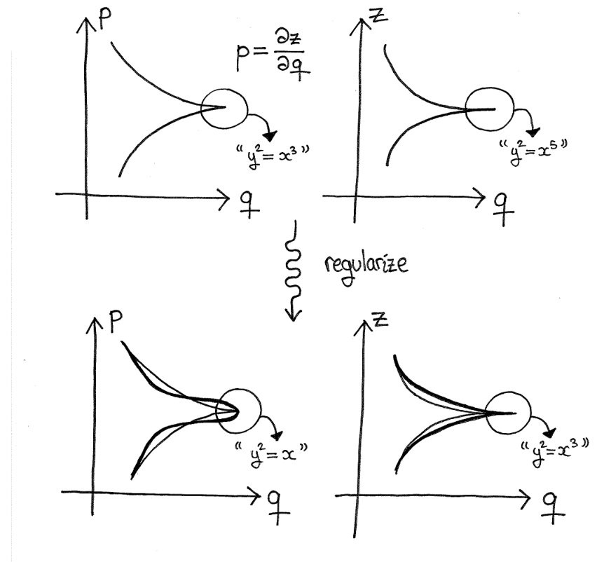
Wrinkles can be regularized as follows. Consider the local model introduced in Section 2.1. Let be a -small function such that on and such that . Let and observe that is a smooth regular embedding such that outside of , see Figure 16.

Next, require further that
whenever , and consider the modified integral
We obtain a regular Lagrangian embedding such that outside of by the formula
The Legendrian counterpart of the regularization is the local model . See Figure 17 for an illustration of the regularization process in the front projection. Given a wrinkled Lagrangian or Legendrian embedding , we can apply this local procedure to every wrinkle and obtain a regular Lagrangian or Legendrian embedding . Similarly, a fibered wrinkled Lagrangian or Legendrian embedding can be regularized to a fibered regular Lagrangian or Legendrian embedding . If is an exact homotopy of wrinkled Lagrangian embeddings, then is an exact homotopy of regular Lagrangian embeddings.

The change in the order of tangency as well as the geometric meaning of the condition can be better appreciated if we focus on the complement of the equator. See Figure 18 for an illustration of the regularization process near a cusp point.
Remark 2.9.
Observe that the regularization process depends on the choice of . However, the space of possible is convex and therefore is well defined up to a contractible choice. Different choices alter by an ambient Hamiltonian isotopy supported on a neighborhood of the image of the wrinkling locus.
Remark 2.10.
In the Lagrangian case, let be foliated by the fibres of the standard projection and in the contact case, let be foliated by the fibres of the front projection . Observe that the standard Lagrangian and Legendrian wrinkles are transverse to these foliations. Moreover, when we regularize the Lagrangian or Legendrian wrinkle we obtain a regular Lagrangian or Legendrian embedding whose singularities of tangency with respect to the corresponding foliation consist of folds away from the equator and of pleats on the equator.
2.6. Sharpening the wrinkles
Let be the north and south hemispheres of the unit sphere and let be the closed unit disk in , which we think of as sitting in via the inclusion . The standard Lagrangian wrinkle is equivalent on to the following local model on .
Note that is the product of and the zero section . By scaling the model by any small number in the direction of the cotangent fibres we get a sharpened Lagrangian cusp . Explicitly, we set
It will be useful for us later on to sharpen the cusps of a Lagrangian wrinkle. This sharpening can be achieved by interpolating between the two models and . The key property of the sharpening construction is that the interpolation can be achieved by a -small perturbation. The precise result that we will need is the following, where we recall the notation , .
Lemma 2.11.
For any there exists an exact homotopy such that the following properties hold.
-
.
-
when or .
-
when and .
-
for some constant independent of and .
The same Lemma also holds for the Legendrian cusp , where . We prove the Lagrangian and Legendrian versions simultaneously.
Proof.
Let be a function satisfying the following properties.
-
for ,
-
for ,
-
for .
We also demand, as we may, that the following bounds hold for some constant independent of and .
-
.
-
.
Finally, we may also choose such that when .
Set and . The front generates the Lagrangian and Legendrian cusps and respectively. To be explicit, we have
The first three properties stated in the Lemma are clearly satisfied. The fourth property follows from the uniform bounds on the first and second partial derivatives of . ∎

Next we explain how to sharpen the birth/deaths of zig-zags on the equator of each wrinkle. The standard Lagrangian wrinkle is equivalent on to the following local model on .
We remark that is the product of with the zero section . For any , the sharpened model is given by
The following result allows us to interpolate between and while maintaining control throughout the perturbation.
Lemma 2.12.
For any there exists an exact homotopy such that the following properties hold.
-
.
-
when or .
-
when and .
-
for some constant independent of and .
As before, the same Lemma also holds for the Legendrian counterpart and we prove both versions simultaneously.
Proof.
Let be a function satisfying the following properties.
-
for ,
-
for ,
-
for .
We again demand that the following bounds hold for a constant independent of and .
-
.
-
.
Moreover, we may also choose such that if .
Set and . The front generates the Lagrangian and Legendrian birth/deaths of zig-zags and respectively. To be explicit, we have
The first three properties stated in the Lemma are clearly satisfied. The fourth property follows from the uniform bounds on the first and second partial derivatives of . ∎

Remark 2.13.
The sharpening construction can also be applied to a family of wrinkled Lagrangian or Legendrian embeddings. To do this, one needs to work instead with the local model for the fibered wrinkle and repeat the above construction in the fibered setting. The proofs only differ in notation.
3. Lagrangian and Legendrian rotations
3.1. Tangential rotations
In Section 1.5 we introduced the notion of a tangential rotation, which decouples a Gauss map from its underlying Lagrangian or Legendrian embedding . We repeat the definition below for convenience. Recall that denotes the Lagrangian Grassmannian of a symplectic or contact manifold .
Definition 3.1.
A tangential rotation of a regular Lagrangian or Legendrian embeddings is a compactly supported deformation , , of such that .
We will also need to consider tangential rotations of wrinkled Lagrangian and Legendrian embeddings. As in the unwrinkled case, a tangential rotation of a wrinkled Lagrangian or Legendrian embedding is a compactly supported deformation , , of such that .
3.2. Simple tangential rotations
Let be a tangential rotation of a possibly wrinkled Lagrangian or Legendrian embedding . A priori, the one-parameter family of Lagrangian planes could rotate around wildly inside . It will be useful for us to restrict these rotations to be of a particularly simple type. See Figure 21 for an illustration of the desired simplicity.
Definition 3.2.
A tangential rotation of a possibly wrinkled Lagrangian or Legendrian embedding is simple if there exists a field of -dimensional planes defined along some open subset such that
-
on we have for all .
-
on the rotation is constant.
We say that is simple with respect to .
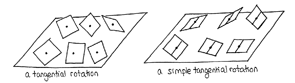
If is regular, then we can think of as a hyperplane field in . When is wrinkled we need to be a little bit careful near the wrinkling locus so it will be best to think of as an ambient -plane field in .
Remark 3.3.
Our definition of simple tangential rotations is slightly more restrictive than the definition given by Eliashberg and Mishachev in [15] for the smooth analogue of this notion. This is the case because the Lagrangian or Legendrian wrinkling model that we are able to construct below is less general than the model used in their proof.
We will also need the notion of piecewise simplicity. A tangential rotation of a regular Lagrangian or Legendrian embedding is piecewise simple if we can subdivide the time interval so that the following property holds. We demand that there exist -plane fields defined along open subsets such that outside of and on for all . We will prove below that any tangential rotation of a regular Lagrangian or Legendrian embedding can be -approximated as accurately as desired by a piecewise simple tangential rotation. In order to do this we first translate the notion of a tangential rotation into the language of jet spaces.
3.3. Rotations of -jets
Let be a regular Lagrangian embedding. Fix once and for all a Riemannian metric on . For small enough, the Weinstein theorem guarantees the existence of a symplectomorphism between a neighborhood of in and , where . We call the Weinstein parametrization. The zero section corresponds under to the embedding . More generally, for any open subset and any function such that , the section corresponds under to a regular Lagrangian embedding which is graphical over .

Similarly, if is a regular Legendrian embedding, then for some small enough there exists a contactomorphism between a neighborhood of in and , which is equipped with the standard contact structure. We still call the Weinstein parametrization. For any open subset and any function such that and , we obtain a regular Legendrian embedding which is graphical over . The embedding corresponds under to the section .
In order to capture the tangential information contained in -jets we must consider -jets. The Riemannian metric fixed on induces the following trivialization of the -jet space .
where is a linear form and is a quadratic form. Explicitly, given a germ of a function , we set . We obtain a vector bundle , where the linear structure is induced by the above trivialization.
Example 3.4.
When with the standard Euclidean metric and standard coordinates , we have a canonical identification for each . Under this identification, and for all .
Definition 3.5.
A -jet rotation of is a compactly supported deformation , , of the zero section which is of the form for some family of quadratic forms .
In other words, a -jet rotation is a deformation of the zero section whose -jet component is zero at all times. The corresponding notion of simplicity for -jet rotations is the following.
Definition 3.6.
A -jet rotation is simple if there exists a hyperplane field defined along an open subset containing such that for all . We say that is simple with respect to .
Remark 3.7.
Observe in particular that has rank . However, the condition of simplicity is stronger, we demand that the kernel always contains a fixed -dimensional distribution. See Figure 23 for an illustration of -jet simplicity.

In the same vein, we say that a -jet rotation is piecewise simple if there exists a subdivision of the time interval such that on each subinterval we have for some simple -jet rotation .
Remark 3.8.
The proper language for this discussion would naturally extend our definitions to include the concepts of - and -holonomic sections of the -jet bundle associated to any fibre bundle. These ideas were introduced by Gromov in [26] in the context of convex integration. We explore these notions further in the context of holonomic approximation in our paper [1], the results of which will be crucially used below.
Given a regular Lagrangian or Legendrian embedding , a Weinstein parametrization of a neighborhood of in and a -jet rotation , we can define a tangential rotation of associated to and . Explicitly, we set at each point , where is any function germ such that and is the Lagrangian or Legendrian embedding corresponding to under . Observe that if is simple, then is also simple.
Conversely, given a regular Lagrangian or Legendrian embedding , a Weinstein parametrization and a tangential rotation of , there exists a unique -jet rotation such that . To be more precise, might only be defined in a small time interval , since the Lagrangian planes could at some point stop being graphical over with respect to , see Figure 24.
Definition 3.9.
When is defined for all , we say that is graphical.
The Weinstein parametrization is implicit in the definition. Observe again that if is simple, then is also simple. The notions of piecewise simplicity also coincide under this correspondence.

3.4. Approximation by simple rotations
Let denote the unit -dimensional cube. The following lemma will allow us to replace any tangential rotation of a Lagrangian or Legendrian embedding by a piecewise simple tangential rotation.
Lemma 3.10.
Let be a -jet rotation such that on . Then there exists a piecewise simple -jet rotation which is -close to and such that on .
Lemma 3.10 is an immediate consequence of a more general approximation result which we prove in [1]. For completeness we present below the outline of the argument in our concrete setting. The idea goes back to Gromov’s iterated convex hull extensions in [26], which used similar decompositions into so-called principal subspaces. Indeed, in convex integration one is also forced to work one pure partial derivative at a time. These decompositions are studied carefully in Spring’s book [39].
For our purposes, we only need to remark that any homogeneous degree polynomial can be written as a sum of squares of linear polynomials. Explicitly, we have the polynomial identity . We can think of a -jet rotation as a parametric family of Taylor polynomials which are homogeneous of degree . By applying the above identity we obtain a decomposition , where the -jet rotation is simple with respect to the hyperplane field and the sum is taken over all . Moreover, it follows that if on , then on for all .

Once we have this decomposition, we can subdivide the interval very finely and add a fraction of each at a time to obtain the desired piecewise simple approximation of . The parametric version is proved in the exact same way. The statement reads as follows.
Lemma 3.11.
Let be a family of -jet rotations parametrized by a compact manifold such that on and such that for . Then there exists a family of piecewise simple -jet rotations which is -close to , such that on and such that for .
To be more precise, for the piecewise simple family we demand that there exists a single subdivision of the time interval such that every is simple on each piece . We can translate Lemmas 3.10 and 3.11 from the world of jet spaces back into the world of symplectic and contact topology. The precise consequence that we wish to extract is the following.
Proposition 3.12.
Let be a tangential rotation of a regular Lagrangian or Legendrian embedding . Then we can -approximate as much as desired by a piecewise simple tangential rotation .
Proof.
By using a partition of unity and a fine enough subdivision of the interval , we can localize in space and time to obtain a tangential rotation which is -close to and such that on each subinterval the rotation is constant outside of some ball . In the Lagrangian case, let be a symplectic isomorphism of the symplectic vector bundle such that . In the Legendrian case, we ask that satisfies the same property but is instead a symplectic isomorphism of the symplectic vector bundle , where on the ball .
Consider the tangential rotation , . Observe that on . By further subdividing the time interval if necessary, we may assume that is graphical. In other words, corresponds to a -jet rotation such that on . Lemma 3.10 asserts the existence of a piecewise simple -jet rotation which is -close to and such that on . We obtain a corresponding piecewise simple tangential rotation which is -close to and such that on . Set , on . Outside of we extend by setting , which is constant for . This piecewise definition yields a tangential rotation , , where each piece is itself a piecewise simple tangential rotation. Hence is also a piecewise simple tangential rotation. Moreover, is everywhere -close to , hence also to . ∎
Remark 3.13.
From the proof we can also deduce the relative version of Proposition 3.12. If on for some closed subset , then we can arrange it so that on .
The parametric version is proved in the same way. The corresponding relative version also holds. As in the case of -jet rotations, by a family of piecewise simple tangential rotations we mean a family of tangential rotations such that for some subdivision of the time interval , every tangential rotation of the family is simple on each subinterval . The precise statement that we will need reads as follows.
Proposition 3.14.
Let be a family of tangential rotations of regular Lagrangian or Legendrian embeddings parametrized by a compact manifold such that for . Then we can -approximate the family as much as desired by a family of piecewise simple tangential rotations such that for .
4. Wiggling embeddings
4.1. Regular approximation near the -skeleton
Let be a tangential rotation of a regular Lagrangian or Legendrian embedding . It is in general impossible to globally -approximate by the Gauss maps of an exact homotopy of regular Lagrangian or Legendrian embeddings , . However, it is always possible to achieve this approximation in a wiggled neighborhood of any reasonable subset of which has positive codimension, see Figure 26. For simplicity, we will restrict ourselves to the following class of stratified subsets.
Definition 4.1.
A closed subset is called a polyhedron if it is a subcomplex of some smooth triangulation of .
In [1] we prove several refinements of the holonomic approximation lemma. The following result is a straightforward application of our holonomic approximation lemma for -holonomic sections.
Theorem 4.2.
Let be a polyhedron of positive codimension and let be a tangential rotation of a regular Lagrangian or Legendrian embedding . Then there exists an exact homotopy of regular Lagrangian or Legendrian embeddings , , such that is -close to on .

Remark 4.3.
We can arrange it so that is -close to on all of and so that outside of a slightly bigger neighborhood of in . Moreover, the result also holds in relative and parametric forms.
Remark 4.4.
As far as the author can tell, Theorem 4.2 does not follow formally from Eliashberg and Mishachev’s holonomic approximation lemma [14] or from any of the other standard -principle techniques. However it does follow immediately from the holonomic approximation lemma for -holonomic sections which we established in [1]. The added difficulty stems from the pervasive danger of cutoffs in symplectic topology.
In Section 5 we will prove that any tangential rotation can be globally -approximated by the Gauss maps of an exact homotopy of wrinkled Lagrangian or Legendrian embeddings . This is the main technical ingredient in the proof of the -principle for the simplification of singularities in Section 6 below. In the course of the proof of this global -approximation theorem we will need to use a result of the same flavour as Theorem 4.2, taking to be the -skeleton of a smooth triangulation of . The idea is to construct the homotopy by first wiggling near the -skeleton. Then one can apply a wrinkling construction on each of the top dimensional simplices to complete the approximation.
However, on the nose Theorem 4.2 is not quite sufficient for our purposes. The issue is that the local wrinkling model which we construct in Section 5 can only be applied if the tangential rotation is simple. Initially this is not a problem because we can use Proposition 3.12 to first approximate any given rotation by a piecewise simple rotation. We can then attempt to deal with each simple piece in the decomposition separately, working step by step. Unfortunately the following additional and subtler difficulty arises. When at each step we apply Theorem 4.2 near the -skeleton of we might find that our fixed decomposition is no longer piecewise simple with respect to the wiggled embedding . If this is the case, then we cannot continue on to the next step. To fix this issue we need a stronger version of Theorem 4.2 which allows us to control the wiggles with respect to a given simple tangential rotation. We phrase and prove this stronger version in the next section, stated as Theorem 4.5.
4.2. Keeping things simple
The precise result that we need is the following application of our holonomic approximation lemma for -holonomic sections from [1]. The choice of a Riemannian metric on and a Weinstein parametrization of a neighborhood of in is implicit throughout. We use the language of -jet rotations introduced in Section 3.3.
Theorem 4.5.
Let be a polyhedron of positive codimension and let be a graphical simple tangential rotation of a regular Lagrangian or Legendrian embedding . Then there exists a graphical simple tangential rotation of and an exact homotopy of regular Lagrangian or Legendrian embeddings , , such that the following properties hold.
-
is -close to on
-
is -close to on all of .
-
is simple with respect to the same hyperplane field as .
-
and outside of a slightly bigger neighborhood of in .
Remark 4.6.
Observe that the second property implies that is everywhere -close to .
Remark 4.7.
The relative form of Theorem 4.5 also holds. If on for some closed subset , then we can arrange it so that and on .
Proof.
By definition of graphicality, we can think of as a -jet rotation which is simple with respect to some hyperplane field . We can therefore apply the (-parametric) holonomic approximation lemma for -holonomic sections from [1] to . The output is a family of functions , and an isotopy such that the following properties hold.
-
is -close to on .
-
is -small on all of .
-
is -small on all of .
-
is -small.
-
is -close to .
-
and outside of a slightly bigger neighborhood of in .
The -smallness of allows us to think of (in the Lagrangian case) or of (in the Legendrian case) as an exact homotopy of regular Lagrangian or Legendrian embeddings . We define the simple tangential rotation by specifying its corresponding simple -jet rotation as follows. Write for a family of quadratic forms and set to obtain the desired , where is the orthogonal projection with kernel . All the properties listed in Theorem 4.5 hold. ∎
The condition that is -close to was not used in this proof but will be used below so we include it for future reference. The above argument also works for families. In the parametric case, we note that the polyhedron may also vary with the parameter. To be more precise, we have the following definition.
Definition 4.8.
A closed subset is called a fibered polyhedron if it is a subcomplex of a smooth triangulation of which is in general position with respect to the fibres , .
A consequence of this definition is that for every the subset given by is a polyhedron in . If has positive codimension in , then has positive codimension in for all . The parametric version of Theorem 4.5 is proved in the same way, by adding a parameter in the notation everywhere and invoking our parametric holonomic approximation lemma for -holonomic sections from [1]. The statement reads as follows. We note that the relative version also holds, as in Remark 4.7.
Theorem 4.9.
Let be a fibered polyhedron of positive codimension and let be a family of graphical simple tangential rotations of regular Lagrangian or Legendrian embeddings parametrized by a compact manifold such that for . Then there exists a family of graphical simple tangential rotations of and a family of exact homotopies of regular Lagrangian or Legendrian embeddings , , such that the following properties hold.
-
is -close to on .
-
is -close to on all of .
-
is simple with respect to the same hyperplane field as .
-
and outside of a slightly bigger neighborhood of in .
-
and for .
4.3. Wiggling the wrinkles
In this section we extend Theorems 4.5 and 4.9, which were stated for regular Lagrangian or Legendrian embeddings, to the case of wrinkled Lagrangian or Legendrian embeddings. In the wrinkled case, we cannot invoke our holonomic approximation lemma for -holonomic sections from [1] directly because a wrinkled Lagrangian or Legendrian embedding is not regular near the wrinkles. The sharpening construction described in section 2.6 will allow us to resolve this issue, since the sharper the wrinkles, the better they can be approximated locally by a regular Lagrangian or Legendrian submanifold..
Given a wrinkled Lagrangian or Legendrian embedding , recall that the subset on which is wrinkled consists of a disjoint union of finitely many -dimensional embedded spheres . Each sphere has an -dimensional equator on which has birth/deaths of zig-zags. The complement consists of two hemispheres on which has cusps.
We say that a polyhedron is compatible with the wrinkles of if the following condition holds. We demand that the wrinkling locus is contained in the -skeleton of and that the union of the equators is contained in the -skeleton of . In the same way we can define what it means for a fibered polyhedron to be compatible with the fibered wrinkles of a family of wrinkled Lagrangian or Legendrian embeddings parametrized by a compact manifold .
We now prove the analogue of Theorem 4.5 for wrinkled Lagrangian and Legendrian embeddings. The precise statement is the following.
Theorem 4.10.
Let be a polyhedron of positive codimension which is compatible with the wrinkles of a wrinkled Lagrangian or Legendrian embedding . Let be a graphical simple tangential rotation of . Then there exists a graphical simple tangential rotation of and a family of exact homotopies , , of wrinkled Lagrangian or Legendrian embeddings such that all of the properties listed in Theorem 4.5 hold.
Proof.
Consider first a single wrinkle in the wrinkling locus of . The wiggling on is performed in two steps. First we will wiggle near the equator and then we will wiggle near the remaining part of . In both cases this wiggling is achieved by replacing the singular Lagrangian or Legendrian submanifold with a regular approximation to which holonomic approximation can be applied. We then use the resulting ambient Hamiltonian isotopy to induce a wiggling of . We will restrict our attention to the Lagrangian case for the sake of concreteness, but the Legendrian case is no different.
In Section 2.6 we introduced the Lagrangian local model for the birth/death of zig-zags. Recall that is given by
Near the equator , our wrinkled Lagrangian embedding is locally equivalent to near . Working in this local model, we can think of as a tangential rotation of which is simple with respect to an -plane field . Consider the zero section , which is a Lagrangian cylinder. Observe that , and moreover that . Extend to , a tangential rotation of which is simple with respect to .
Let and set . Apply Theorem 4.5 to the regular Legendrian embedding , the simple tangential rotation and the stratified subset . We obtain an exact homotopy of regular Legendrian embeddings which we may assume is constant outside of . Recall that is -close to near . Recall also that is everywhere -close to a tangential rotation which is also simple with respect to and which is supported on .
Write for an ambient Hamiltonian isotopy which we may assume constant outside of . Let and consider the sharpening of described in Section 2.6 with respect to the parameters and . Recall that for some constant independent of and , so by taking small enough we may replace with from the onset up to an error which is proportional to . Recall also that sharpening is supported on and is -sharp on . For details see Section 2.6.
Consider now . Note that on the Gauss map of this composition is -close to . Indeed, and are tangent along and when we invoke Theorem 4.5 to construct we can demand as much accuracy in the approximation as we want. Next, observe that is supported on and on that neighborhood is -close to a tangential rotation which is simple with respect to . Let denote the standard projection. As in the sharpening , for each the tangent plane converges to the horizontal plane tangent to the zero section at the point , and hence converges to . It follows that by taking as small as is necessary, we can use to exhibit a tangential rotation of which is simple with respect to and which is arbitrarily -close to on all of . We have therefore achieved the required global approximation up to an error which is proportional to . Since we can take to be arbitrarily small, this completes the wiggling near the equator.
Once we have wiggled near the equator we proceed to wiggle on the two hemispheres of the complement . Near the interior of each of the two disks and the map is equivalent to the local model on , where we recall from Section 2.6 that
Our input this time is a simple tangential rotation of the local model which we assume to be constant on . The strategy is the same as before. Consider the zero section and extend to a simple tangential rotation of . Then apply (the relative version of) Theorem 4.5 to , and to obtain an exact homotopy of regular Lagrangian embeddings which is induced by an ambient Hamiltonian isotopy fixing the boundary. For a suitable choice of parameters and , the concatenation of the sharpening homotopy described in Section 2.6 followed by the isotopy gives the required wiggling on
The analogue of the parametric Theorem 4.9 for families of wrinkled Lagrangian or Legendrian embeddings also holds, where we demand that the fibered polyhedron is compatible with the wrinkles. The proof only differs in notation and the precise statement reads as follows.
Theorem 4.11.
Let be a fibered polyhedron of positive codimension which is compatible with the wrinkles of a family of wrinkled Lagrangian or Legendrian embeddings parametrized by a compact manifold . Let be a family of graphical simple tangential rotations of such that for . Then there exists a family of graphical simple tangential rotations of and an exact homotopy of wrinkled Lagrangian or Legendrian embeddings , , such that all of the properties listed in Theorem 4.9 hold.
Remark 4.12.
5. Wrinkling embeddings
5.1. Wrinkled approximation on the whole manifold
As we already mentioned, we cannot in general hope to globally -approximate a tangential rotation of a regular Lagrangian or Legendrian embedding by the Gauss maps of a homotopy of regular Lagrangian or Legendrian embeddings. In the previous section, we showed that the approximation can nevertheless be achieved by such a regular homotopy in a small neighborhood of any polyhedron of positive codimension. In this section we show that the approximation can be globally achieved on the whole manifold if we allow the homotopy to be wrinkled. See Figure 28 for an illustration. More, precisely we have the following theorem, which is the main result of this section.
Theorem 5.1.
Let be a tangential rotation of a regular Lagrangian or Legendrian embedding . Then there exists a compactly supported exact homotopy of wrinkled Lagrangian or Legendrian embeddings , such that is -close to .

Theorem 5.2.
Let be a graphical simple rotation of a wrinkled Lagrangian or Legendrian embedding . Then there exists a compactly supported exact homotopy of wrinkled Lagrangian or Legendrian embeddings , such that is -close to .
The parametric version of Theorem 5.1 reads as follows.
Theorem 5.3.
Let be a family of tangential rotations of regular Lagrangian or Legendrian embeddings parametrized by a compact manifold such that for . Then there exists a family of compactly supported exact homotopies of wrinkled Lagrangian or Legendrian embeddings , such that is -close to and such that for .
As in the non-parametric case, by Proposition 3.14 we can reduce Theorem 5.3 to the following statement.
Theorem 5.4.
Let be a family of graphical simple rotations of wrinkled Lagrangian or Legendrian embeddings parametrized by a compact manifold such that for . Then there exists a family of compactly supported exact homotopies of wrinkled Lagrangian or Legendrian embeddings , such that is -close to and such that for .
The proof of Theorems 5.2 and 5.4 consists of two steps. The first step is the construction of a local wrinkling model, which we carry out in Section 5.2. The second step is to combine this local wrinkling model with the wiggling results established in Section 4 to obtain the desired global approximation. We carry out this second step in Section 5.3.
5.2. Local wrinkling model
We begin by describing the local model for the oscillating function that will generate the wrinkles. This is essentially the same local model used by Eliashberg and Mishachev in [15]. In fact, our local wrinkling model for Lagrangians and Legendrians is obtained from theirs by simply integrating and differentiating the formulae, just like we did in Section 2 with the definition of wrinkled Lagrangian and Legendrian embeddings.
The basic geometric idea behind the construction is quite straightforward. One wishes to wrinkle the Lagrangian or Legendrian submanifold back and forth so that the wrinkles are parallel to the rotating planes . Since we model the wrinkles on a highly oscillating function, the Gauss map of the resulting wrinkled embedding gives an arbitrarily good approximation of . There is a delicate part of the construction regarding the embryos of the zig-zags because the oscillating function is forced to have a derivative with the ‘wrong sign’ in some neighboring region. However, we will impose bounds on the size of this bad derivative to ensure that its effect is not significant.
Construction 5.5 (The oscillating function).
First, we fix some notation. We will localize our problem from a general -dimensional manifold to the unit cube . A point will be written as , where . We will consider rotations which are simple with respect to the (constant) hyperplane field spanned by the vectors . Hence the last coordinate will play a special role in our discussion. We will also need a time parameter, which will be denoted by . Sometimes it will be convenient to consider time as another spatial parameter, in which case we will think of the domain of our local model as .
Consider the family of curves , , given by parametric equations
The curve is a graph of a continuous function which is smooth for and smooth on for , where we note that . See Figure 29 for an illustration. We note that the constants and are chosen for convenience in the calculation but are otherwise immaterial.
Remark 5.6.
Observe that the composition is smooth for all .

Let be small and choose an odd -periodic family of functions , , illustrated in Figure 30, which satisfies the following properties.

Let denote the closed unit dimensional disk. We now use the family to define a model which like depends on but also depends on three more parameters and .
Fix a non-increasing function such that
-
for ,
-
for .
Fix a non-increasing cutoff function such that
-
for
-
for near .
Fix also another non-increasing cutoff function such that
-
for
-
for near .
We define our oscillating model by the following formula, see Figure 31 for an illustration.

Given , and , let denote the box
which is a copy of centered at and scaled by and in the and directions respectively. Let be the obvious diffeomorphism obtained by translating and rescaling. Define . The oscillating function also depends on the parameters , and . We will call and the top and bottom of the box respectively. We will also need to consider the slightly smaller boxes
Observe that has wild oscillations on which die out on , so that is smooth on and on .
Finally, we modify our local model to make it Lagrangian. We do this by integrating and differentiating as in the definition of wrinkled Lagrangian embeddings. Define by the formula
Observe that is defined in terms of , hence also depends on the parameters and . Observe also that is odd in the variable, hence on . It follows that has a Legendrian lift which agrees with the zero section on .
Given any box we can similarly define a translated and scaled version of which has support in . This completes the construction of our local wrinkling model.
Remark 5.7.
The function is not smooth and hence is also not smooth. However, can be smoothly reparametrized and therefore so can . We will revisit this nuance later on but it will not cause us any trouble.
We are now ready to state and prove the local wrinkling lemma. Note that a tangential rotation of the inclusion of the zero section is simple with respect to the hyperplane field if it can be written as
for some angle function . According to our previous definition we say that is graphical when . We will say that is quasi-graphical when .

Lemma 5.8 (Local wrinkling for Lagrangians).
Let be a tangential rotation of the zero section which is quasi-graphical and simple with respect to and such that on . Then there exists an exact homotopy of wrinkled Lagrangian embeddings , , such that the following properties hold.
-
is -close to .
-
on .
Proof.
Let be small. We will be precise about exactly how small we need to be later on. Wrinkling is dangerous and unnecessary where is close to zero, so we will first use our oscillating model to define a similar model which does not oscillate on the subset of in which .
Remark 5.9.
Although we want to think of time as a spatial parameter, observe that on the boundary face , so we are not quite in the relative setting. To remedy this, we extend the time interval from to by setting for . We can then work with the box as our local model, which has the advantage that on . We can later restrict back to only considering times and forget about the rest.
Let . We call a box special if for near the top and bottom of . Choose special boxes which are contained in and such that the smaller boxes are still special and cover . This can be achieved if is sufficiently small and is sufficiently big. Write for the parametrizing diffeomorphisms as above. We can assume that the sets are disjoint. Therefore for each integer there exists a number such that for all the subsets
are also disjoint. When we let below, we will let accordingly so that we always have .
For each box we have an oscillating Lagrangian model . Let . Define the Lagrangian oscillating model adapted to by setting . More precisely, we set
Observe that and outside of . At this point we can restrict back to the time interval , which is all that we really cared about.
Consider the Hamiltonian function given by . For each we get a Hamiltonian isotopy such that the vector field is the symplectic dual of . Hence we have
It follows by explicit computation that
We set . Note that on since . Note moreover that on we have
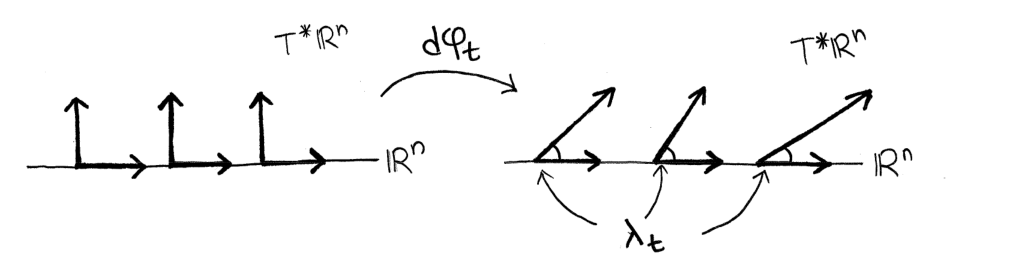
Hence in particular on we have
Set . We recall from Remark 5.7 that each is not smooth, hence is not smooth, hence the same is true for . However, we can precompose with a reparametrization of the domain so that and hence also is smooth. Note moreover that this reparametrization does not change the image of and therefore it also doesn’t change the image of the Gauss map , which is what we actually care about. By abusing notation we will also use to denote the reparametrized smooth map whenever this is convenient. See Figures 34 and 35 for an illustration of .


Claim 5.10.
For any we can choose parameters and so that .
We recall the parameters at play. The game is all about controlling the different rates at which the parameters tend to zero or infinity, so it will be important to be precise in the interdependence of the parameters and in the order of quantifiers.
-
is the cutoff angle of under which we will perform no wrinkling.
-
is proportional to the the width of the shell between a box and the smaller box .
-
is the order of magnitude of on the regions where it is large and negative (inside the wrinkles).
-
controls the magnitude of the ‘bad’ negative derivative when the wrinkles die out.
-
is the height of the oscillating model .
-
is proportional to the number of wrinkles in .
We begin by fixing arbitrarily small. To choose , observe that
and hence if , then the scalar product of and is positive and moreover we have
Recall that on the subset we have . Suppose that . It follows that if , then we have
Once is fixed, we choose small enough so that the construction of (which depends implicitly on ) is possible. The other parameters must be chosen somewhat more judiciously. Our first task is to understand the geometry of the initial local model in order to control the error produced when we modify the model to make it Lagrangian.
Consider the Lagrangian version in given by the formula
where we recall that
We also have the corresponding scaled version
If and in such a way that , then the Gauss map converges (on compact subsets of the plane) to the distribution spanned by the vectors and . The proof is the following explicit computation.
It will we convenient to carry out our calculations in terms of the function and its derivative . Note that the zero set is precisely the wrinkling locus of . We compute:
and hence provided that we have
With some minor modifications we can extend our computations to the scaled dimensional model for the Lagrangian wrinkle as it appears in .
where . Indeed, the only difference comes from the terms for and their partial derivatives, which give an error that tends to zero as and . The conclusion is that provided we have , the Gauss map converges to the distribution
Recall that we must ensure so that the singularity loci are disjoint. Hence if we let , then we must also allow for . But this only helps us in the above computation so there is no issue.
Consider next the oscillating model defined above. Let be the locus on which is not smooth. The set consists of a disjoint union of spheres with cuspidal equators. Let be the compact region bounded by . If and so that , then the above computations show that on the Gauss map of converges to the distribution . In the complement of , the model is smooth and for we have as . On the subset the Gauss map of converges to , indeed on the remaining part the derivative is strictly positive and scales by while scales by for . On we cannot control so precisely but we assert that outside of there still holds the following lower bound:
To confirm this assertion, we compute
Since and in the region where , the first term is always non-negative. For the second term we use our assumption that and the desired inequality follows.
We deduce from this inequality that if we let and so that and , then on the complement of we have . Of course we also still have for , and as .
Next we proceed to study the model which is adapted to our rotation . Assume first for simplicity that , so that for all . Let be the non-smooth locus of . The set is again a disjoint union of spheres which have cuspidal equators. Let be the compact subset bounded by . Note that . On all the derivatives are bounded below by a positive constant times and at each point there is at least one of them which is bounded below by a constant times . This last assertion holds because the boxes cover . Inside all the derivatives are bounded above by a positive constant times and at each point there is exactly one derivative for which is bounded above by a constant times . This last derivative corresponds to the whose non-smooth locus bounds the given component of containing the point we’re looking at. We recall that we are letting with the only requirement that . Hence if and in such a way that this condition holds and if additionally we have and , then on the region the Gauss map of converges to the distribution and on and on we know that for and that gets arbitrarily close to the sector
Consider next the general case where we don’t assume that for all . Since is a disjoint union, we can repeat the above reasoning on each component and reach the same conclusion, provided that we modify that definition of the subset as follows
We now return to the wrinkled Lagrangian embedding . Recall that along the zero section the linear symplectic isomorphism is the map which sends
so that along the zero section. Recall also that we chose so that on we have for all . Under the above convergence assumptions it follows that we have on and hence also . Therefore on . Outside of we have . If we assume that on the Gauss map of converges to the distribution , then for we have
The analogous result for Legendrians is stated and proved in the same way. Observe as in the Lagrangian case that a tangential rotation of the inclusion of the zero section is simple with respect to the hyperplane field if it can be written as
for some function . According to our previous definition we say that is graphical when . We will say that is quasi-graphical when .
Lemma 5.11 (Local wrinkling for Legendrians).
Let be a tangential rotation of the zero section which is quasi-graphical and simple with respect to and such that on . Then there exists an exact homotopy of wrinkled Legendrian embeddings , , such that the following properties hold.
-
is -close to .
-
on .
Proof.
We proceed exactly like we did in the proof of Lemma 5.8. The Legendrian model is simply given by the Legendrian lift of the Lagrangian model which exists because of the exactness condition on . ∎
The parametric versions read as follows. Note that we also localize the problem from a general -dimensional parameter space to the unit cube .
Lemma 5.12 (Parametric local wrinkling for Lagrangians).
Let be a family of tangential rotations of the zero section parametrized by the unit cube which are all quasi-graphical and simple with respect to , such that on and such that for . Then there exists a family of exact homotopies of wrinkled Lagrangian embeddings , , such that the following properties hold.
-
is -close to .
-
on .
-
for .
Lemma 5.13 (Parametric local wrinkling for Legendrians).
Let be a family of tangential rotations of the zero section parametrized by the unit cube which are all quasi-graphical and simple with respect to , such that on and such that for . Then there exists a family of exact homotopies of wrinkled Legendrian embeddings , , such that the following properties hold.
-
is -close to .
-
on .
-
for .
Lemmas 5.12 and 5.13 are proved in the same way as Lemmas 5.8 and 5.11, adapting our construction to the fibered case as in [15]. To be more precise, in the local model for the oscillating function we replace the box by the box and set
The rest of the proof can then be repeated carrying the parameter along for the ride.
5.3. Wrinkling the wiggles
We are now ready to prove that tangential rotations can be globally approximated by Gauss maps of wrinkled embeddings.
Proof of Theorem 5.2.
Let be a graphical simple rotation of a wrinkled Lagrangian or Legendrian embedding . Let be a triangulation of which is compatible with the wrinkles of as in Section 4.3. Set , the -skeleton of . By Theorem 4.10, there exists an exact homotopy of wrinkled Lagrangian or Legendrian embeddings , , (which is in fact an isotopy in the sense of Remark 4.12) and a tangential rotation of such that the following properties hold.
-
is -close to on .
-
is -close to on all of .
-
is graphical and simple with respect to the same hyperplane field as .
-
and outside of a slightly bigger neighborhood of in .
Take an open simplex in , so that is an exact homotopy of regular Lagrangian or Legendrian embeddings. Replace the hyperplane field by a constant hyperplane field, so that we reduce to the model , . The error in the approximation can be made arbitrarily small by first subdividing the triangulation as finely as is necessary. There exists a tangential rotation covering the exact homotopy such that the following properties hold.
-
is -close to .
-
is quasi-graphical and simple with respect to .
-
on .
The rotation is nothing other than from the point of view of the deformed embedding . Hence we can apply our local wrinkling Lemma 5.8 or 5.11 to obtain an exact homotopy of wrinkled Lagrangian or Legendrian embeddings such that the following properties hold.
-
is -close to
-
on .
The local wrinklings glue up to an exact homotopy of wrinkled Lagrangian or Legendrian embeddings such that is -close to . The proof is complete. For an illustration of the argument, see Figure 36. ∎

The proof of the parametric Theorem 5.4 follows the same outline, using the parametric Theorem 4.9 instead of Theorem 4.5 and using the parametric Lemmas 5.12 and 5.13 instead of Lemmas 5.8 and 5.11. The only essential difference is that in order to localize the parameter space from an arbitrary -dimensional manifold to the unit cube we need to choose a triangulation of which is compatible with the wrinkles of and such that every simplex in the triangulation is in general position with respect to the fibres , . The existence of such a triangulation was proved by Thurston in [43]. Once we know that such a triangulation exists, we can take the fibered polyhedron and work simplex by simplex.
6. The simplification of singularities
6.1. Wrinkles, swallowtails and double folds
We now return to the setting described in Section 1. Let be a symplectic or contact manifold and let be a foliation of by Lagrangian or Legendrian leaves. Suppose that is a winkled Lagrangian or Legendrian embedding which is transverse to . We can apply the regularization procedure described in Section 2.5 to and obtain a regular Lagrangian or Legendrian embedding . We already observed in Remark 2.10 that only has -type singularities with respect to , see Figure 37 for an illustration. More precisely, consists of a disjoint union of regularized wrinkles, which are defined as follows.
Definition 6.1.
A regularized wrinkle of a regular Lagrangian or Legendrian embedding is a connected component of the singularity locus which consists of a topologically trivial codimension sphere such that we can decompose into two hemispheres and and an equator satisfying the following.
-
the equator consists of pleats.
-
the disks and consist of folds.
For a concrete local model, one can take the standard Lagrangian or Legendrian wrinkle defined in Section 2.2, after regularizing as described in Section 2.5. In the Lagrangian case, the foliation of the cotangent bundle is given by the fibres of the standard projection . In the Legendrian case, the foliation of the -jet space is given by the fibres of the projection .
Remark 6.2.
If the foliation is induced by a Lagrangian fibration , then for any regular Lagrangian embedding the following two conditions are equivalent.
-
the singularities of tangency of with respect to consist of a union of regularized wrinkles.
-
the front is a generalized wrinkled mapping in the sense of [15].
In the contact case where is a Legendrian fibration (which we think of as the front projection), we can think of regularized wrinkles in the following way. The singularities of tangency of a regular Legendrian embedding consist of a union of regularized wrinkles if and only if the front of the embedding has cusps on each sphere together with swallowtails on the equator of each .
Regularized wrinkles are also close relatives of the double folds introduced in Section 1.3. We recall the definition for convenience.
Definition 6.3.
A double fold is a pair of topologically trivial -spheres and in the fold locus which have opposite Maslov co-orientations and such that is the boundary of an embedded annulus .
Indeed, the Entov surgery of [19] can be used to open up a regularized wrinkle along its equator, producing a double fold. This is achieved by taking one of the two hemispheres of a regularized wrinkle and pushing it slightly away from while keeping it fixed on the equator . We obtain an embedded disk contained in an arbitrarily small neighborhood of in such that and . In fact, we require that is outside of the -ball bounded by . The surgery construction removes the pleats from and trades them for folds on two parallel copies of . One of these two parallel copies of is surgered onto one of the hemispheres of and the other parallel copy is surgered onto the other hemisphere, so that the end result consists of a disjoint union of two parallel spheres on which the embedding has folds. The Maslov co-orientations on the two resulting spheres are opposite of each other. Hence we end up with the desired double fold. See [19] for the details of the surgery construction and see Figure 38 for an illustration.

The precise statement that we will need is the following. Given a regular Lagrangian or Legendrian embedding and given a regularized wrinkle, there exists a -small ambient Hamiltonian isotopy such that outside of an arbitrarily small neighborhood of in and such that inside this neighborhood the regularized wrinkle of is replaced by a double fold of . If is the regularization of a wrinkled Lagrangian or Legendrian embedding , then the wrinkles of will typically be nested. By this we mean that the ball bounded by any wrinkle of may contain other wrinkles of . Hence when we apply the surgery construction on each regularized wrinkle of , we obtain a regular Lagrangian or Legendrian embedding whose singularity locus consists of a disjoint union of double folds which are nested in the sense of Section 1.3.
Remark 6.4.
We could of course have worked with double folds all along without ever mentioning wrinkles. Instead of defining wrinkled Lagrangian and Legendrian embeddings as we did, we could have defined ‘doubly cusped’ Lagrangian and Legendrian embeddings to be smooth Lagrangian or Legendrian embeddings away from a finite union of pairs of parallel spheres where the embedding has cusps of opposite Maslov co-orientation (the cusps are semi-quintic in the ambient symplectic or contact manifold and semi-cubic in the front projection).
Our -approximation result for a tangential rotation would also hold for the class of doubly cusped Lagrangian and Legendrian embeddings. Moreover, the regularization of a doubly cusped Lagrangian or Legendrian embedding which is transverse to a foliation is a regular Lagrangian or Legendrian embedding whose singularities of tangency with respect to consist of double folds. The -principle for the simplification of singularities proved below then follows with the same proof.
We have chosen to work with wrinkles for two reasons. One is historical, to draw the parallel with the smooth wrinkled embeddings theorem [15]. The second is pedagogic, since wrinkling is not only a central notion in flexible geometric topology but also the main idea in our proof, so hiding it in the background would be dishonest.
Suppose next that is a family of wrinkled Lagrangian or Legendrian embeddings parametrized by a compact manifold . We can also in this case regularize and obtain a family of regular Lagrangian or Legendrian embeddings . If is transverse to , then the singularities of tangency of the family with respect to consist of fibered regularized wrinkles. In particular, for some values of the parameter the regular Lagrangian or Legendrian embedding will have regularized embryos in addition to regularized wrinkles. Regularized embryos are non-generic -type singularities of tangency which occur at the instance of birth/death of a regularized wrinkle. One can of course give a concrete local model for the regularized embryo, however it is simpler to think about families as a single object using the fibered terminology. For a concrete local model, one can take the standard fibered Lagrangian or Legendrian wrinkle defined in Section 2.3, after regularizing as described in Section 2.5. The foliation is given as in the non-parametric case.
Remark 6.5.
If the foliation is induced by a Lagrangian fibration , then for any family of regular Lagrangian embeddings the following two conditions are equivalent.
-
the singularities of tangency of with respect to consist of a union of fibered regularized wrinkles.
-
the fibered front is a fibered generalized wrinkled mapping in the sense of [15].
In the Legendrian case one can of course reinterpret what fibered regularized wrinkles mean in the front projection in terms of cusps and swallowtails. Note that one can also use the Entov surgery in families to replace fibered regularized wrinkles with fibered double fold singularities. The embryos of regularized wrinkles will become embryos of double folds. An embryo of a double fold is a non-generic locus of -type singularities of tangency consisting of a single codimension sphere from which the two parallel spheres of folds can either be born or die, see Figure 39.

6.2. The -principle for the simplification of singularities
We are now ready to establish the flexibility of singularities of Lagrangian and Legendrian fronts. As above, denotes a foliation by Lagrangian or Legendrian leaves of a symplectic or contact manifold .
Theorem 6.6.
Suppose that there exists a tangential rotation of a regular Lagrangian or Legendrian embedding such that . Then there exists a compactly supported ambient Hamiltonian isotopy such that the singularities of consist of a union of nested regularized wrinkles.
Proof.
Apply the wrinkling Theorem 5.1 to and . We obtain a compactly supported exact homotopy of wrinkled Lagrangian or Legendrian embeddings such that . Next, apply the regularization process described in Section 2.5 to the homotopy . We obtain a compactly supported exact homotopy of regular Lagrangian or Legendrian embeddings such that the singularity locus consists of a disjoint union of regularized wrinkles. Finally, since the homotopy is exact and compactly supported, we can write for some compactly supported ambient Hamiltonian isotopy . ∎
To deduce the version with double folds stated in Theorem 1.11, we simply apply the Entov surgery construction of [19] to open up each of the wrinkles as described in the previous section.
Remark 6.7.
At each stage of the proof, when we apply Theorem 5.1, the regularization of Section 2.5 and the Entov surgery, we can always ensure that the resulting homotopy of embeddings is -close to . Hence Theorem 6.6 also holds in -close form, where we demand that the Hamiltonian isotopy is -close to the identity . Moreover, we can also ensure that outside of a neighborhood of in .
Remark 6.8.
Suppose that on for some closed subset . At each stage of the proof, when we apply Theorem 5.1, the regularization of Section 2.5 and the Entov surgery, we can always ensure that the resulting homotopy of embeddings agrees with on . Hence Theorem 6.6 also holds in relative form. More precisely, we can demand that on .
The parametric version reads as follows, and is proved in exactly the same way. At each stage we just need to invoke the parametric versions of each of the ingredients of the proof. The corresponding -close and relative versions also hold, for the same reasons as in the non-parametric case.
Theorem 6.9.
Suppose that there exists a family of tangential rotations of regular Lagrangian or Legendrian embeddings parametrized by a compact manifold such that for all and such that for . Then there exists a family of compactly supported ambient Hamiltonian isotopies such that the singularities of consist of a union of fibered nested regularized wrinkles and such that for .
As in the non-parametric case we can open up the fibered regularized wrinkles into fibered double folds using the Entov surgery construction [19].
Remark 6.10.
Observe that in the case there is no need to resolve a wrinkle into a double fold. Indeed a -dimensional regularized wrinkle consists of nothing more than a pair of points where the embedding has folds of opposite Maslov co-orientation. For fibered regularized wrinkles the two folds die as in the Legendrian Reidemeister I move. We explore the case further in Section 6.5 below.
6.3. The -principle for the prescription of singularities
We next prove a strengthened version of Entov’s Theorem 1.14. More precisely, we apply our -principle Theorem 6.6 to drop the -nonsingularity restriction from his result. As an application we establish some concrete results for the simplification of the caustics of spheres in Section 6.4 below.
Consider a Lagrangian or Legendrian embedding and let be a Lagrangian distribution in defined along . In the symplectic case, consists of linear Lagrangian subspaces of and in the contact case consists of linear Lagrangian subspaces of , where locally .
When for all we say that is -nonsingular. In this case, the structure of the singularity locus is quite simple. Indeed, for generic nonsingular the locus is a codimension submanifold which is naturally stratified as a flag as described in Section 1.3. Moreover, the flag comes equipped with certain co-orientation data which we hinted about in Section 1.9 and which more precisely consist of the following.
-
Unit vector fields , , where each is defined on , is normal to in and cannot be extended (as such a unit normal vector field) to any subset which has a nontrivial intersection with .
-
An additional unit vector field defined on the whole of which is normal to in . This vector field is called the Maslov co-orientation.
Adapting Eliashberg’s terminology from [9], Entov defined in [19] the chain of singularities associated to and to consist of the flag together with vector fields as above. The are uniquely determined by the geometry of the singularity. See Figure 40 for an illustration. Two chains of singularities are said to be equivalent if there exists an isotopy of that transforms one into the other, including the co-orientation data. We can now state and prove an -principle which allows for the prescription of any homotopically allowable chain of singularities. The result also holds in -close and relative forms.

Theorem 6.11.
Let be a regular Lagrangian or Legendrian embedding into a symplectic or contact manifold equipped with a foliation by Lagrangian or Legendrian leaves. Let be a homotopy of Lagrangian distributions defined along , fixed outside of a compact subset, such that and such that is -nonsingular with respect to the distribution . We moreover assume that outside of that compact subset. Then there exists a -small compactly supported Hamiltonian isotopy such that is -nonsingular with respect to and moreover such that the chain of singularities of with respect to is equivalent to the chain of singularities of with respect to , together with a union of nested double folds.
Proof.
We restrict our attention to the Lagrangian case for concreteness, the Legendrian analogue is no different. Let be the singularity locus of with respect to . By abusing notation, we will also denote by the chain of singularities which encodes the flag and the corresponding co-orientation data. Let be a homotopy of linear symplectic isomorphisms of defined along such that and . Set , a tangential rotation of .
Our plan will be the following. We will first apply our holonomic approximation lemma for holonomic sections to to make transverse to near a parallel copy of . Then we will introduce by hand a cancelling pair of singularity loci and in such that is equivalent to and such that bounds an embedded annulus which is disjoint from . Formally, and can be cancelled via a rotation which is fixed on and hence by our relative principle for the simplification of singularities we are able to keep the singularity locus and fill in the rest of the Lagrangian submanifold with double folds. See Figure 41 for an illustration of the strategy.

Let , which is a line field on defined along . Extend to a tubular neighborhood of in . Denote by the parallel copy of in . Apply Theorem 4.2 to the tangential rotation and the stratified subset . We obtain an exact homotopy of regular Lagrangian embeddings such that is -close to on . In particular, on a neighborhood of .
Along , the Lagrangian distributions and are transverse. We can therefore choose a symplectic isomorphism such that the horizontal distribution (which is tangent to the zero section) is mapped to using and such that the vertical distribution (which is tangent to the cotangent fibres) is mapped to . Choose an -dimensional complement for in . Set and , where denotes orthogonality with respect to the symplectic form . Let be a function satisfying the following properties.
-
for near .
-
for near .
-
for and for .
Fix nonzero vector fields and . Define a homotopy of Lagrangian distributions defined along by the formula
Note that , that on and that for all . The singularities of tangency of with respect to the zero section consist of two parallel copies and of , for concreteness say is between and . Along these singularitiy loci we have . The two corresponding chains of singularities, which we also denote by and , have opposite Maslov co-orientations but are otherwise equivalent. Replacing the function by the function if necessary, we may assume that the chain of singularities is equivalent to the chain .
At this point we wish to use to insert by hand a cancelling pair of singularities modelled on . The explicit formulas that we need are already written down in Entov’s paper [19]. We could use these formulas to write down a concrete model for the creation of the cancelling pair, but we can make our life even easier by directly applying Entov’s Theorem 1.14 to . The output of Entov’s theorem is an exact homotopy of regular Lagrangian embeddings such that is the inclusion of the zero section , such that is fixed on and such that the singularities of tangency of with respect to are equivalent to those of with respect to , together with a union of nested double folds. Furthermore, the homotopy can be assumed to be -small, so by taking an appropriate Weinstein neighborhood we can think of this homotopy as happening inside . The result is an exact regular homotopy of such that along the singularities of tangency of with respect to consist of a union , where the chain is equivalent to , the chain is equivalent to and is a union of nested double folds. Moreoever, bounds an annulus which is disjoint from .
Claim 6.12.
There exists a tangential rotation of which is fixed on and such that away from .
Once this claim is established we are done, since we can apply the relative version of Theorem 6.6 to construct an exact homotopy of regular Lagrangian embeddings which is fixed on and such that at the end of the homotopy the singularities of tangency away from consist of a union of nested double folds, which is exactly what we wanted to prove.
To justify the claim, we first observe that there exists a tangential rotation of such that is fixed on , such that outside of and such that away from . To define , choose such that the annuli contain . Inside of , we let kill the double folds of so that the only remaining singularities are . On the rest of (where we may assume that provided that and are close enough to ), we construct in three steps.
-
First, rotate to a distribution which equals away from and which interpolates between and on by means of .
-
Since is -close to on , we can then rotate to a distribution which equals away from , which interpolates between and on by means of and which then interpolates between and on .
-
We can then rotate to a distribution which equals outside of and which interpolates between and on . The distribution satisfies the required properties and the rotation is the concatenation of the three steps.
Consider now the annulus with boundary . The intersection consists of two line fields defined over the images of and . We claim that they extend to a line field defined over the image of the whole annulus .
Indeed, the chain of singularities of is equivalent to that of up to Maslov co-orientation. But the isotopy class of the line field which arises from a -type singularity locus is completely dictated by the flag together with the non-Maslov co-orientation data. Hence the line fields are isotopic in . It follows that we can find a line field defined along such that and such that .
Suppose that there exists a family of symplectic isomorphisms of such that , such that , such that near and such that near . Then the line field is the required extension. It remains to confirm that the family exists. We need to define over , where and we have prescribed over . Furthermore, we also have prescribed the image of under the map over all of . Since this map is a Serre fibration, it follows that we can find a lift to all of . This completes the proof of the existence of the line field .
Next we observe that the distribution satisfies and . Pick a complement to . Set and . Pick nonzero vector fields and such that on and define a rotation starting at by the formula
Observe that on we have and hence for all . Hence we can extend outside of by letting it equal elsewhere. Observe also that along and hence . Recall that is a two-sided hypersurface of , so that if is a small enough neighborhood of , then has exactly two connected components. The fact that the Maslov co-orientations of and are opposite means precisely that lies in the same connected component of . Hence we can push the image of entirely off of by a small deformation which is fixed outside of . The result is a rotation starting at such that on and such that away from . This completes the proof of Claim 6.12, hence also of Theorem 6.11. ∎
6.4. Application: the caustics of spheres
We now return to the first example considered in Section 1.1. Our goal is to study the extent to which it is possible to simply the caustic of an embedded Lagrangian or Legendrian sphere , where is a symplectic or contact manifold equipped with a foliation by Lagrangian or Legendrian leaves. For greater clarity of the exposition we will restrict our discussion to the Lagrangian version of the problem, but the Legendrian analogue is no different.
First we observe that by the Weinstein neighborhood theorem we can immediately reduce to the case where and is the image of the zero section , which we will also denote by . Note that for the problem is uninteresting because the generic caustic consists only of folds, so the simplification of singularities can be trivially achieved. We assume in what follows. Let be the restriction to of the distribution of Lagrangian planes tangent to . We begin with the following topological obstruction to the simplification of singularities.
Proposition 6.13.
If is Hamiltonian isotopic to a Lagrangian sphere whose singularities of tangency with respect to consist only of folds, then is stably trivial as a real vector bundle over the sphere.
We precede the proof with some notation. Let be any compact hypersurface. Following [17], it is conceptually useful to introduce a real -dimensional vector bundle which is obtained from by regluing along with a fold. More precisely, write for two compact -dimensional submanifolds whose common boundary is the hypersurface . Fix also an identification , where denotes the trivial line bundle. Define to be the real -dimensional vector bundle over given by gluing the disjoint union over the intersection via the isomorphism

The bundle can be realized as a distribution of Lagrangian planes in defined along the zero section whose singularities of tangency with respect to the zero section consist of folds along . In order to do this, we fix a co-orientation of , which will agree with the Maslov co-orientation induced by . Let be a tubular neighborhood of such that the canonical orientation of the interval induces the chosen co-orientation of . The Lagrangian Grassmannian is the trivial circle bundle . We use the canonical coordinates . Let be the rotating line field defined over the zero section by the formula

Define to be the distribution of Lagrangian planes defined over the zero section which corresponds to the product of the cotangent fibres of and the line field under the isomorphism . The distribution extends to the complement of in by letting it consist of the cotagent fibres of on . The real vector bundle underlying is isomorphic to .
Proof of Proposition 6.13.
We first consider the special case where itself has only fold singularities with respect to . Then the caustic is an embedded hypersurface in co-oriented by the Maslov co-orientation. A direct consequence of the local model for the fold is that and are homotopic in the space of Lagrangian distributions. Since the real vector bundle underlying is isomorphic to , it remains to show that is stably trivial. To see this, observe that is obtained from and by using the gluing along , where we still think of as . Nothing changes if instead we use the gluing , since the two linear isomorphims of given by and are in the same connected component of . We can therefore define a bundle map by sending via the inclusion , by sending via the map and by gluing the two pieces into a global map using . This glued up map is an isomorphism, hence , as claimed.
Consider now the general case where is a Hamiltonian isotopy such that only has fold singularities with respect to . Equivalently, only has fold singularities with respect to the pullback foliation . From the special case already considered it follows that the restriction to of the distribution must be stably trivial as a real vector bundle over the sphere. But and are homotopic as distributions of Lagrangian planes and therefore isomorphic as real vector bundles. Hence is also stably trivial. ∎
We now use our -principle for the prescription of singularities to show that for even, the necessary condition for the simplification of singularities provided by Proposition 6.13 is also sufficient.
Corollary 6.14.
Assume that is even and that is stably trivial as a real vector bundle over the sphere. Then there exists a compactly supported Hamiltonian isotopy such that the singularities of tangency of with respect to consist only of folds. Moreover, we can take to be -close to the identity and supported on an arbitrarily small neighborhood of the zero section.
Remark 6.15.
From the proof we can also extract a precise description of the permissible fold loci as hypersurfaces of in terms of the Euler number of . The locus can be arranged to consist of the boundary of any -dimensional compact submanifold of Euler characteristic , together with a disjoint union of nested double folds.
Proof.
If is a closed embedded ball, it is readily seen that is the trivial bundle. Fix a trivialization . We obtain a trivialization by identifying both bundles with . Suppose that is chosen so that is transverse to along . Then with respect to this trivialization the distribution determines a class , where is the Grassmannian of linear Lagrangian subspaces of and we choose any as a basepoint. Let be the image of under the map given by long exact sequence in homotopy groups associated to the fibration . Observe that is the clutching function corresponding to the real vector bundle underlying the distribution . Note that the choice of ball induces a choice of orientation on , which is encoded in the class .
The stable triviality of means that is in the kernel of the map , where is the stable orthogonal group. However, is an isomorphism as soon as , and therefore , where the map is given by the long exact sequence in homotopy groups associated to the fibration . Recall that under this map the fundamental class is sent to the clutching function corresponding to the tangent bundle . We can therefore write for some .
Let by any compact hypersurface disjoint from . Let and be as in the construction of , so that and . We choose the labels so that , and then we agree to orient so that the inclusion is orientation preserving. It is straightforward to compute the Euler class using for example the Poincaré-Hopf index theorem. Since , if we choose the hypersurface so that , then it follows that and are isomorphic as oriented real vector bundles.
Using the same construction as above, we can exhibit as a distribution of Lagrangian planes in defined along the zero section . Observe that the singularities of tangency of the zero section with respect to the distribution consist of folds along .
Since is even, and hence we have an injection . Observe that the homotopy classes in determined by the distributions and have the same image under this map. It follows that and are homotopic in the space of Lagrangian distributions. The -principle for the prescription of singularities Theorem 6.11 applies to produce a -small Hamiltonian isotopy supported in a neighborhood of the zero section such that the singularities of tangency of with respect to are equivalent to those of with together with a union of nested double folds, which completes the proof. ∎
In fact, the assumption that is stably trivial is automatically satisfied for all even such that mod . One can argue in the following way. Choose a class , which we think of as the clutching function of a real vector bundle. By exactness of the long exact sequence in homotopy groups associated to the fibration , it is equivalent to ask that is in the image of the map or to ask that it is in the kernel of the map . The first condition says that the vector bundle can be realized as a distribution of Lagrangian planes in defined along the zero section , while the second condition says that the complexification of the vector bundle is trivial. Suppose that is such a class and let be the image of under the stabilization map induced by the inclusion . By commutativity of the diagram below, observe that lies in the kernel of the map .
However, , since both homotopy groups lie in the stable range. This kernel can be computed from Bott periodicity. Indeed, implies that and therefore the groups appearing in the exact sequence depend on the residue class of mod as follows.
| mod | |||
|---|---|---|---|
From the table we deduce that except if or mod (in which case the kernel is isomorphic to ). It follows that if is even and mod , then we necessarily have , as claimed.
Remark 6.16.
The simplest example of a caustic that cannot be simplified to consist only of folds occurs when and is the Hopf bundle on . It is easy to check that in this case a pleat is unavoidable, in addition to the folds.
When is odd, the same reasoning still shows that a necessary and sufficient condition for the simplification of singularities to be possible is that is homotopic to one of the standard models in the space of Lagrangian distributions. However, stable triviality of the underlying real vector bundle is not sufficient to guarantee that this condition is satisfied because and hence the map need not be an injection.
We have only touched the surface of the homotopy theoretic calculations which are necessary to understand the formal condition obstructing the simplification of caustics. In the very concrete example of spheres considered above we were able to reason in a fairly hands-on manner. We believe that it should be possible to carry out a more systematic approach in the spirit of obstruction theory to study the general case.
6.5. Application: families of -dimensional Legendrians
We now turn to the second application discussed in Section 1.1. Our goal is to establish that higher singularities are unnecessary for the homotopy theoretic study of the space of Legendrian knots in the standard contact Euclidean . Recall that we think of as the jet space which comes equipped with the contact form . The Lagrangian projection is the map , which corresponds to the forgetful map . The front projection is the map , which corresponds to the forgetful map . The Reeb direction is and it will also be useful to think of the projection along the Reeb direction which is the map .
The fibres of the front projection form a Legendrian foliation of . Recall that a Legendrian knot is said to have mild singularities when the only singularities tangency of with respect to are folds and embryos. Folds are the generic singularities of a single Legendrian knot and in the front projection correspond to cusps, see Figure 44. Embryos are the generic singularities of a -parametric family of Legendrian knots and in the front projection correspond to Type I Reidemeister moves, namely the instances of birth/death of two cusps. See Figure 45.


Generically, a Legendrian knot only has folds and a -parametric family of Legendrian knots only has folds and embryos. However, the caustic of a family of Legendrian knots parametrized by a space of high dimension will generically be very complicated. It is therefore not a priori clear how the topology of the space of Legendrian knots is related to that of the subspace consisting of those Legendrian knots whose singularities are mild. In Section 1.1 we defined a space of decorations and a space of pairs consisting of a Legendrian knot with mild singularities together with a decoration of the singularities of . See Figure 46 for an example of a decoration compatible with the standard front projection of the figure eight knot.

By composing the forgetful map given by with the inclusion we obtain a map . In this section we will prove the following result, which is a consequence of our parametric -principle for the simplification of caustics.
Corollary 6.17.
The map is a weak homotopy equivalence on each connected component.
Remark 6.18.
The decoration is necessary because the inclusion is not a homotopy equivalence, indeed . To see this, let be a family of Legendrian knots parametrized the closed unit -disk which has mild singularities everywhere except for a single singularity appearing in the interior. Then it is easy to see that the family represents a nontrivial element of . The decoration is designed to kill this homotopy group.
Remark 6.19.
If is any Legendrian knot, then by a generic perturbation we may assume that the singularities of consist only of a finite number of folds. Then is compatible with the trivial decoration consisting of and . It follows that is surjective. However, is it easy to see that is not injective, since in the space we are keeping track of the decoration .
To prove Corollary 6.17 it suffices to show that for and that is surjective. We deal with each of the statements separately.
Proof that for .
Let be any class. We can represent by a map such that lifts to a map . To conclude that we must show that there exist a homotopy which is fixed on and such that extends to a lift of .
We begin by examining the singularity locus of on the boundary, which is the subset consisting of all pairs such that the front of the Legendrian knot has a fold or embryo singularity at the point . Denote the map which forgets the knot but remembers the decoration by . The family of decorations induces a decomposition of the singularity locus , where consists of folds and consists of pairs of folds with opposite Maslov co-orientations together with the embryos that give rise to the birth/death of such pairs. The folds of correspond to the points and the pairs of folds or embryos of correspond to the endpoints of the intervals . Note that the number of intervals may vary with the parameter but the number of points is fixed since . After a generic perturbation we may assume that and are smooth codimension submanifolds of and moreover that the set of embryos is a smooth codimension submanifold of .
Our strategy is the following. The first step is to construct near the boundary of the parameter space . This involves manually killing all the pairs of folds in . The next step is to extend the folds in to the interior of the parameter space . After these two preparatory steps we can apply the relative form of our parametric -principle to construct everywhere else so that the only additional singularities of the deformed family are the folds and embryos resulting from the wrinkling process. By construction the resulting map will have an obvious lift to , completing the proof.
We now perform the first of these preparatory steps. The key idea, which appears repeatedly throughout the literature of the wrinkling philosophy, is that to kill a zig-zag one may create a very small new zig-zag near one end of the old zig-zag and then slowly let the new zig-zag take over, eventually killing the old zig-zag and replacing it. The newly created zig-zag does not bother us because it will end up completely contained in the interior of the parameter space .
Fix a collar neighborhood of , which we parametrize radially as with corresponding to . It will be convenient to assume that is radially invariant on , and indeed by means of an initial homotopy of fixed on the boundary we can arrange it so that for all and all . Note then that and moreover . For an satisfying this condition we establish the following preparatory result.
Lemma 6.20 (Preliminary arrangement near the boundary).
There exists a homotopy of such that the following properties hold.
-
is fixed on .
-
.
-
The folds in are left untouched throughout the homotopy. To be more precise, the subset does not vary with time.
-
The pairs of folds in are killed at the end of the homotopy. To be more precise, over each cylinder the singularity locus contains arcs whose interiors lie in and whose endpoints lie in and in fact consist precisely of the endpoints of the intervals . Moreover, each arc consists everywhere of folds except at a single point in its interior, which is an embryo.

Proof.
To construct the homotopy we will use the parameter family of Legendrian fronts exhibited in Figure 47. Suppose that is a non-degenerate interval appearing in the decoration for some . Assume moreover that is isolated, meaning that there are no other intervals contained inside or containing . In a neighborhood of the front of the knot is equivalent to either the local model or to a flip of in the vertical direction, depending on the Maslov co-orientations. By replacing by the vertical flip of whenever this is needed, we may assume without loss of generality that the former case holds.
Note that the family of fronts can be made to be -close to the constant family , so that the resulting Legendrian isotopy is -small. We can therefore think of the parameter family as a Legendrian isotopy of supported on .
It is conceptually useful to understand the projection of the family along the Reeb direction. The front projects down to a zig-zag. As the parameter increases from to , a new zig-zag is created just outside of . We then make this new zig-zag bigger and bigger, until it takes over and replaces the old zig-zag, which has died by the time that is close to . This process is illustrated in Figure 48

To define formally, let be a function such that the following properties hold.
-
on .
-
on .
-
is non-decreasing on and non-increasing on .
We define the homotopy on by the formula . Suppose next that there are two nested intervals with no other interval either contained or containing or . Then we define the homotopy just like we did before, but using a nested version of the family which we exhibit in Figure 49. For more complicated configurations of intervals we repeat this strategy but using the obvious model which is obtained by nesting the parameter family (or its flip in the vertical direction) according to the nesting of the configuration of intervals.


The construction described above can be realized parametrically as varies, as long as no interval degenerates to a point. However, in a neighborhood of the locus of embryos we need a different local model so that the family does not degenerate into a higher singularity. The -parametric family exhibited in Figure 50 gets the job done. Let us first understand what the locus looks like in a neighborhood of . Fix a connected component and set . Consider the image of under the projection . Note that is a smooth codimension submanifold with boundary, that is the image of , that the map is a to cover away from and that along the map has folds. In particular, the restriction is an embedding, see Figure 51.

Let be a collar neighborhood of in such that . Given , let be its image in and let , correspond to the arc . Then the -parametric family is equivalent in a neighborhood of the embryo point to the -parametric family exhibited at the top row of Figure 50 (or to its flip in the vertical direction).
Observe that the family can be taken to be -close to the family which is constant in . We can therefore think of the -parametric family as a -small Legendrian isotopy of the -parametric family supported in a neighborhood of the embryo point. Notice that , so the isotopy is compatible with our previous isotopy. Notice also that is constant. We can therefore define the homotopy by the formula , where . The construction can be realized parametrically in , see Figure 52 for an illustration. The construction can also be realized with any configuration of intervals, by nesting the families shown in Figures 49 and 50 according to the nesting of the intervals. This completes the proof of Lemma 6.20. ∎

The next step is to extend the cusp locus to the interior of the parameter space . This is achieved by a second preparatory lemma. For notational convenience, we now forget about our old family and use the letter to denote the new family produced by Lemma 6.20. In particular, all of the properties listed in the conclusion of Lemma 6.20 are satisfied by .
Lemma 6.21 (Preliminary arrangement in the interior).
There exists a homotopy of such that the following properties hold.
-
is fixed on .
-
The singularity locus contains a properly embedded submanifold with boundary of codimension in which consists entirely of folds and such that .
Remark 6.22.
Since is fixed on , also contains the properly embedded codimension submanifold with boundary formed by the arcs which kill . In addition to and , the singularity locus may have other components, but we will not care about them because they are all homotopically trivial and contained in .
Proof.
We assume that , otherwise the Lemma is trivial. Recall that the space of decorations is fibered over the (unordered) configuration space of points on the circle . The map is and its fibers are contractible. Denote by the composition of with the fibration . We claim that the map extends to a map .
First observe that each component of is homotopy equivalent to . Hence for there is nothing to prove because . If , then we need to justify the claim. Write , where is Poincaré dual to and is Poincaré dual to . Consider the Gauss map , , where and we project away the factor. Explicitly, an angle corresponds to the line field spanned by . Observe that . Observe also that the fundamental class of is Poincaré dual to for some , where we recall that is the number of points in the decorations . If we write for the inclusion and denote by the class which is Poincaré dual (PD) to a point, then we have
However, has image generated by . It follows that and hence that is an embedded curve in which is homologous to . Note then that has necessarily components, each of which is homologous to . It is now a triviality to check that extends to a map , as claimed.
Choose then such an extension and assume without loss of generality that is radially constant in the annulus . Choose also a tangential rotation of the family such that the following properties hold.
-
is fixed on .
-
on the subset .
Using the parametric version of theorem Theorem 4.2 (which in the -dimensional case is the same as Theorem 4.9 since all rotations are simple) we obtain a homotopy of the family which is fixed on and such that is -close to on . The family does not quite have folds along , but is almost parallel to on and does have folds along . By implanting the local model for the creation of a pair of folds exhibited in Figure 53 into we can arrange it so that the new family does have folds precisely along . Moreover, we can arrange it so that the new family agrees with the old family inside . Away from the singularities of might be a mess but we don’t care. The proof of Lemma 6.21 is complete.∎

We can now conclude the proof that for . Given represented by a family , we can apply Lemmas 6.20 and 6.21 and replace with the family obtained after performing the two preliminary arrangements, in that order. For the new , we claim the existence of a family of tangential rotations of the family such that the following properties hold.
-
is fixed on
-
away from .
To verify the claim, we begin by considering the restriction of the Gauss map to the annulus . Note that by construction the lift extends to a lift , where we assign intervals to the new pair of folds created by the family . The intervals of the decoration which do not correspond to pairs of folds in give us a homotopically canonical deformation of such that is fixed on and such that away from . Together with the requirement that is fixed near , this defines the map on . Each connected component of the complement of in is diffeomorphic to , where is a closed interval and the diffeomorphism is of the form . Consider the cube
which we think of as a subset of via the above diffeomorphism. See Figure 54. Note that has boundary

The homotopy defined thus far gives a map of pairs , where . Since for , there exists a homotopy of pairs relative to the boundary so that at the end of the homotopy the image is disjoint from . This is precisely what we needed to define on the remaining part of so that the required conditions are satisfied.
Now that we have established the existence of such a tangential rotation , we can invoke Theorem 6.9 to construct a homotopy of which is fixed on and such that away from the singularities of the family consist of a finite union of fibered nested regularized wrinkles. It only remains to show that extends to a lift of to . However, this is clear because to the folds of and to the pairs of folds of we can assign points and intervals in the obvious way, while away from the singularities of consist only of the pairs of points in the fibered regularized wrinkles, to which intervals can be canonically assigned. This completes the proof that for . ∎
Proof that is surjective.
Let be any class. We can represent by a map such that . Choose any decoration which is compatible with . We must show that there exists a homotopy of such that for all and such that lifts to a map with .
Write for points and non-degenerate intervals . Let . Observe that the Gauss map of the family satisfies on . Let be a tangential rotation of the family such that is fixed on and such that on . Using Theorem 4.9 as above, we can construct a homotopy which is fixed near and such that is -close to on .
By the insertion of the local model in Figure 53 we can assume that actually has folds along . Theorem 6.9 can then be used to further homotope rel so that on the complement of the only singularities are fibered nested regularized wrinkles. This new admits a canonical lift by assigning intervals to the pairs of points in the fibered regularized wrinkles. This completes the proof that is surjective. Hence Corollary 6.17 is also proved. ∎
We conclude this section with a remark. Proving that for amounts to solving the following lifting problem. Given a diagram of the form
we must show that there exists a map such that when added to the above diagram all compositions commute up to a homotopy fixed on . The proof of Corollary 6.17 achieves this, but in fact proves slightly more. Because all of the theorems invoked hold in -close form and because all of the local models used are -small perturbations, it follows that the composition of the lift with the map can be taken to be -close to the original map . The analogous -approximation result holds for the corresponding lifting property for proving that is surjective.
6.6. Final remarks
We conclude our discussion with a couple of remarks.
Remark 6.23.
All of the results proved in this paper also hold for immersed rather than embedded Lagrangians or Legendrians . The reason is that from the onset one can replace with or by choosing a Weinstein neighborhood of the immersion, thereby reducing to the embedded case. The only difference in the conclusion is that the resulting exact homotopy of regular Lagrangian or Legendrian immersions will not be induced by an ambient Hamiltonian isotopy in the original manifold .
Remark 6.24.
It is worth giving the following warning. If the singularities of a regular Lagrangian or Legendrian embedding with respect to only consist of a disjoint union of regularized wrinkles (or double folds), then the singularity locus is quite simple in the source. However, in the target the image of the singularity locus is likely to be very complicated. Moreover, this complication is likely to encode most, if not all, of the rigidity of the Lagrangian or Legendrian submanifold.
Remark 6.25.
From Theorems 5.1 and 5.3 we can also deduce a full -principle for directed embeddings of wrinkled Lagrangian or Legendrian embeddings analogous to the one deduced by Eliashberg and Mishachev from their wrinkled embeddings theorem [15]. Before we can state it, we need a definition.
Definition 6.26.
For any Lagrangian or Legendrian embedding and for any subset , we say that is -directed if .
The result is then the following.
Theorem 6.27.
Let be a Lagrangian or Legendrian embedding, let be any open subset and assume that there exists a tangential rotation of such that . Then there exists an exact homotopy of wrinkled Lagrangian or Legendrian embeddings such that is -directed.
References
- [1] Alvarez-Gavela D. Refinements of the holonomic approximation lemma, ArXiv: —– 2015.
- [2] Arnold, V.I. A characteristic class entering in quantization conditions, Functional Analysis. and its Applications, 1:1 (1967), 1-13.
- [3] Arnold V.I. Singularities of Caustics and Wave Fronts, Kluwer Academic Publishers, 1990.
- [4] Arnold V.I. Gusein-Zade S.M. Varchenko A.N.Singularities of Differentiable Maps, Volume I, Springer, 1985.
- [5] Arnold V.I. Gusein-Zade S.M. Varchenko A.N.Singularities of Differentiable Maps, Volume II, Springer, 1988.
- [6] Boardman J.M. Singularities of differentiable maps, Publications Mathématiques de l’I.H.É.S, 33 (1967), no. 2, 21-57.
- [7] Ekholm T. Morse flow trees and Legendrian contact homology in 1-jet spaces, Geometry & Topology. 11 (2007), 1083-1224.
- [8] Eliashberg Y.M. On singularities of folding type Izv. Akad. Nauk SSSR Ser. Mat. (1970) Volume 4, Issue 5.
- [9] Eliashberg Y.M. Surgery of singularities of smooth mappings , Izv. Akad. Nauk SSSR Ser. Mat. (1972) Volume 36, Issue 6.
- [10] Eliashberg Y.M. Mishachev N.M. Wrinkling of smooth mappings and its applications. I, Inventiones mathematicae, 1997.
- [11] Eliashberg Y.M. Mishachev N.M. Wrinkling of smooth mappings. III. Foliations of codimension greater than one, Topological Methods in Nonlinear Analysis, 11 (1998), no. 2, 321-350.
- [12] Eliashberg Y.M. Mishachev N.M. Wrinkling of smooth mappings. II. Wrinkling of embeddings and K. Igusa’s theorem, Topology, 39 (2000), no. 4, 711-732.
- [13] Eliashberg Y.M. Mishachev N.M. Holonomic approximation and Gromov’s h-principle arXiv:math/0101196.
- [14] Eliashberg Y.M. Mishachev N.M. Introduction to the h-principle, Graduate Studies in Mathematics, Volume 48, 2002.
- [15] Eliashberg Y.M. Mishachev N.M. Wrinkled Embeddings, Foliations, geometry, and topology; Contemporary Mathematics, 498 (2009), 207-232.
- [16] Eliashberg Y.M. Mishachev N.M. The space of framed functions is contractible, Essays in mathematics and its applications, 81-109, Springer, Heidelberg, 2012.
- [17] Eliashberg Y.M Mishachev N.M. Topology of Spaces of S-Immersions, Perspectives in Analysis, Geometry, and Topology, Progress in Mathematics Volume 296, 2012, pp 147-167.
- [18] Eliashberg Y.M Galatius S. Mishachev N.M Madsen-Weiss for geometrically minded topologists, Geometry & Topology, 15 (2011), no. 1, 411-472.
- [19] Entov M. Surgery on Lagrangian and Legendrian Singularities, Geometric and Functional Analysis 9:2 (1999), 298-352.
- [20] Entov M. On the Necessity of Legendrian Fold Singularities, IMRN International Mathematics Research Notices 1998, No. 20.
- [21] Emmanuel F. Pushkar’ E.P. Non cancellation of singularities on wave fronts C. R. Acad. Sci. Paris, S?er. I Math. 327 8 (1998) 827?831.
- [22] Emmanuel F. Pushkar’ E.P. Morse theory and global coexistence of singularities on wave fronts Journal of the London Mathematical Society 74, no. 2, 527?544 2006.
- [23] Givental A.B. privative communication, 2017.
- [24] Gromov M.L. Stable maps of foliations into manifolds, Izv. Akad. Nauk SSSR Ser. Mat. (1969) Volume 33, Issue 4.
- [25] Gromov M.L. Convex integration of partial differential relations, Izv. Akad. Nauk SSSR Ser. Mat., 37(1973), 329-343.
- [26] Gromov M.L. Partial Differential Relations, Springer, 1986.
- [27] Hirsch M. Immersions of manifolds, Transactions of the American Mathematical Society, 93(1959), 242-276.
- [28] Igusa K. Higher singularities are unnecessary, Annals of Mathematics, 119(1984), 1-58.
- [29] Igusa K. The space of framed functions, Trans. of Amer. Math. Soc., 301(1987), no 2, 431?477.
- [30] Kragh T. Parametrized Ring-Spectra and the Nearby Lagrangian Conjecture, arXiv:1107.4674. 2011
- [31] Kupers S. Three applications of delooping applied to H-principles arXiv:1701.06788
- [32] Morin B. Formes canoniques des singularites d’une application differetiable C. R. Acad. Sci. Paris 260 1965.
- [33] Murphy E. Loose Legendrian Embeddings in High Dimensional Contact Manifolds, arXiv:1201.2245. 2012.
- [34] Lurie J. On the Classification of Topological Field Theories, arXiv:0905.0465.
- [35] Phillips A. Submersions of open manifolds, Topology, 6(1967), 171-206.
- [36] Rourke C. Sanderson B. The compression theorem I-II Geometry & Topology, 5(2001), 399-429, 431-440.
- [37] Rourke C. Sanderson B. The compression theorem III: applications Algebraic & Geometric Topology, 3, (2003), 857-872.
- [38] Smale S. The classification of immersions of spheres in Euclidean spaces, Annals of Mathematics, (2) 69(1959), 327-344
- [39] Spring D. Convex Integration Theory, Birkhäuser, 1998
- [40] Spring D. Directed embeddings and the simplification of singularities, Communications in Contemporary Mathematics, 4(2002), 107-144.
- [41] Spring D. Directed embeddings of closed manifolds, Communications in Contemporary Mathematics, 7(2005), 707-725.
- [42] Thom R. Les singularités des applications différentiables, Annales de l’Institut Fourier, 6 (1956), no. 6, 43-87.
- [43] Thurston W. The theory of foliations of codimension greater than one, Commentarii Mathematici Helvetici, 49(1974), 214Ð231.