Refinements of the holonomic approximation lemma

We begin by briefly recalling the holonomic approximation lemma, which is the starting point of our paper. Given a fibre bundle $p:X\to M$, where $X$ and $M$ are smooth manifolds, consider the bundle $p^{r}:X^{(r)}\to M$ of $r$-jets of $p$. The fibre of $p^{r}$ over a point $x\in M$ consists of equivalence classes of germs of sections $h:Op(x)\to X$ of $p$, where two germs are identified if they agree up to order $r$ at the point $x$. Throughout we use Gromov’s notation $Op(A)$ to denote an arbitrarily small but unspecified open neighborhood of a subset $A\subset M$. If $X=M\times N$ is a trivial bundle, then sections of $p$ are the same as maps from $M$ to $N$ and we usually write $X^{(r)}=J^{r}(M,N)$.

Given a section $h:U\to X$ of $p$ defined over an open subset $U\subset M$, we denote by $j^{r}(h):U\to X^{(r)}$ the section of $p^{r}$ consisting of the $r$-jets of $h$. Sections of $p^{r}$ of the form $j^{r}(h)$ are called holonomic. It is generally impossible to globally approximate an arbitrary section $s:M\to X^{(r)}$ of $p^{r}$ by a holonomic section. Nevertheless, the approximation can always be achieved in a deformed neighborhood of any reasonable stratified subset of positive codimension. For simplicity we restrict our discussion to the following class of stratified subsets.

The classical holonomic approximation lemma was first stated and proved in [3] by Eliashberg and Mishachev. They give numerous applications in their book [4]. Holonomic approximation is closely related to the method of continuous sheaves discovered by Gromov in his thesis [6] and further explored in his book [8]. Both of these techniques greatly generalize the immersion theory of Smale-Hirsch-Phillips [9], [10], [13]. The precise statement that we wish to recall reads as follows.

The holonomic approximation lemma 1.2 is an extremely useful tool for proving $h$-principles. However, it turns out that for certain applications a stronger statement is needed. The goal of this paper is to prove several refinements of the method of holonomic approximation, which we formulate in this section. In Section 1.3 we state the parametric versions. In Section 1.4 we explain how these refinements yield new flexibility results in symplectic and contact topology.

Recall that for $0\leq l<r$ there are maps $p^{r}_{l}:X^{(r)}\to X^{(l)}$ which forget higher order information. The projection $p^{r}_{l}$ gives $X^{(r)}$ the structure of an affine bundle over $X^{(l)}$. Given a section $s:A\to X^{(r)}$ of $p^{r}$ defined over any subset $A\subset M$, we call $s^{(l)}=p^{r}_{l}\circ s:A\to X^{(l)}$ the $l$-jet component of $s$.

Our first refinement of the holonomic approximation lemma states that if we start with an $l$-holonomic section $s$ of $p^{r}$, then it is possible to carry out the holonomic approximation process on $s$ while ensuring global control of the $l$-jet component.

Our second refinement concerns a specific class of $(r-1)$-holonomic sections of $p^{r}$, which we call $\perp$-holonomic. Informally, we can describe a $\perp$-holonomic section as a section of $p^{r}$ which differs from a holonomic section only by the formal analogue of a pure order $r$ partial derivative. We show that when the holonomic approximation process is applied to a $\perp$-holonomic section it is not only possible to globally control the $(r-1)$-jet component, but it is also possible to globally control the order $r$ information complementary to this formal pure order $r$ partial derivative. The precise statement is most cleanly phrased in terms of the bundle $X^{\perp}$, which we define below. This bundle was first introduced in by Gromov in [8] in the context of convex integration, where the language of $\perp$-jets is used to construct iterated convex hull extensions of partial differential relations. A thorough exposition of the theory of convex integration, including details on the geometry of $X^{\perp}$, can be found in Spring’s book [14].

Let $\tau\subset TM$ be a hyperplane field on $M$. We associate to $\tau$ a bundle $p^{\perp}:X^{\perp}\to M$ in the following way. The fibre of $p^{\perp}$ over a point $x\in M$ consists of equivalence classes of germs of sections $h:Op(x)\to X$ of $p$, where two germs are identified if their $(r-1)$-jets $y=j^{r-1}(h)(x)\in X^{(r-1)}$ at the point $x$ are the same and moreover if the restriction of their tangent maps $d\big(j^{r-1}(h)\big):T_{x}M\to T_{y}X^{(r-1)}$ to the hyperplane $\tau_{x}\subset T_{x}M$ are the same. When $X=M\times N$ is a trivial bundle we also write $X^{\perp}=J^{\perp}(M,N)$. Observe that $X^{\perp}$ lies between $X^{(r)}$ and $X^{(r-1)}$ in the sense that there exist natural affine bundle structures $p^{r}_{\perp}:X^{(r)}\to X^{\perp}$ and $p^{\perp}_{r-1}:X^{\perp}\to X^{(r-1)}$ such that $p^{\perp}_{r-1}\circ p^{r}_{\perp}=p^{r}_{r-1}$. Given a section $s:A\to X^{(r)}$ of $p^{r}$ defined over any subset $A\subset M$, we call $s^{\perp}=p^{r}_{\perp}\circ s:A\to X^{\perp}$ the $\perp$-component of $s$. Given a section $h:U\to X$ of $p$ defined over an open subset $U\subset M$, we denote by $j^{\perp}(h):U\to X^{\perp}$ the section of $p^{\perp}$ formed by the $\perp$-jets of $h$. Explicitly, $j^{\perp}(h)=p^{r}_{\perp}\circ j^{r}(h)$. Sections of $p^{\perp}$ of the form $j^{\perp}(h)$ are called holonomic.

Our main results Theorem 1.5 and Theorem 1.8 remain true in families. We take our parameter space to be a compact manifold $Z$, whose boundary $\partial Z$ is possibly nonempty. We consider families of sections parametrized by $Z$. For example, a family of sections $s_{z}:M\to X^{(r)}$ depending on the parameter $z\in Z$ is a smooth mapping $s:Z\times M\to X^{(r)}$ such that for every $z\in Z$ the assignment $x\mapsto s(z,x)$ defines a smooth section $s_{z}$ of $p^{r}$. Additionally, we allow the polyhedron $K$ to vary with the parameter in the following way.

A consequence of this definition is that for every $z\in Z$ the subset $K_{z}\subset M$ given by $K\cap(z\times M)=z\times K_{z}$ is a polyhedron in $M$, see Figure 4. If $K$ has positive codimension in $Z\times M$, then $K_{z}$ has positive codimension in $M$ for all $z\in Z$. We are now ready to formulate the parametric analogues of Theorems 1.5 and 1.8.

We begin with an example which illustrates the main point. Suppose that $f:L^{n}\to W^{2n}$ is a Lagrangian embedding of a manifold $L$ into a symplectic manifold $(W,\omega)$. Denote by $\pi:\Lambda_{n}(W)\to W$ the Grassmannian bundle of Lagrangian planes in $TW$. The fibre of $\pi$ over a point $x\in W$ consists of the linear Lagrangian subspaces of the symplectic vector space $(T_{x}W,\omega_{x})$. The Gauss map $G(df):L\to\Lambda_{n}(W)$ of the embedding $f$ is defined by $G(df)(q)=df(T_{q}M)\subset T_{f(q)}W$.

By compactly supported we mean that $G_{t}=G(df)$ for all $t\in[0,1]$ outside of a compact subset of $L$. The following approximation result is a simple corollary of our holonomic approximation lemma for $l$-holonomic sections.

If we attempt to prove Theorem 1.15 using the classical holonomic approximation lemma 1.2 instead, we run into the following difficulty. The functions $h_{t}$ produced by the holonomic approximation would a priori only be defined in open subsets $Op\big(F_{t}(K)\big)\subset L$. We would therefore need to extend $h_{t}$ to the whole of $L$ by hand. The most straightforward way of doing so is to choose a family of cutoff functions $\psi_{t}:L\to\mathbb{R}$ supported on the domain of $h_{t}$ such that $\psi_{t}=1$ near $F_{t}(K)$. The product $\widetilde{h}_{t}=\psi_{t}\cdot h_{t}:L\to\mathbb{R}$ is then well defined on all of $L$. It follows that the composition $f_{t}=d\widetilde{h}_{t}\circ F_{t}:L\to T^{*}L$ is an exact homotopy of Lagrangian embeddings whose Gauss map provides the desired approximation near $K$.

If $||d\widetilde{h}_{t}||<\delta$ on all of $L$, then $f_{t}$ has image contained in $T^{*}_{\delta}L$ and we can think of $f_{t}$ as an exact homotopy of Lagrangian embeddings $f_{t}:L\to W$ as before. Observe, however, that there is no guarantee that $d\widetilde{h}_{t}=\psi_{t}dh_{t}+h_{t}d\psi_{t}$ has norm $<\delta$, because $\psi_{t}$ will typically have a very large derivative. Indeed, the wiggling $F_{t}$ is quite dramatic, see Figure 6 for an illustration. Therefore, $f_{t}(L)$ might escape outside of our Weinstein neighborhood $T^{*}_{\delta}L\simeq\mathcal{N}$. Hence $f_{t}$ does not correspond to an exact homotopy of Lagrangian embeddings into $W$ and our proof breaks down. Our holonomic approximation lemma for $l$-holonomic sections with $l=1$ precisely provides the necessary global control on the $1$-jet component so that this issue does not arise.

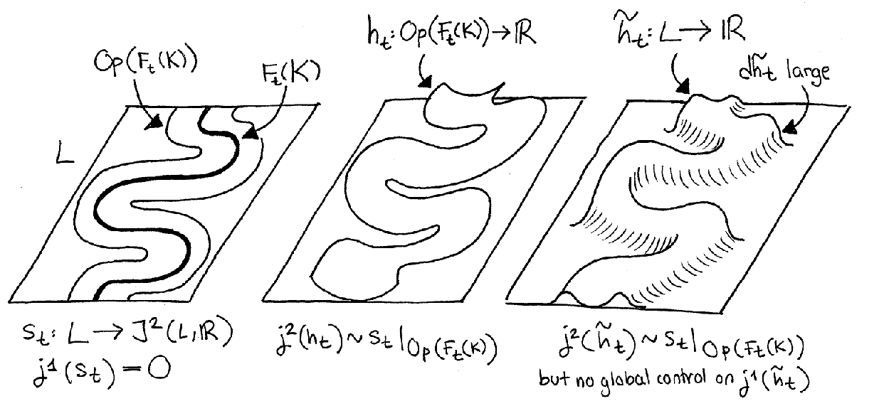
The parametric version of Theorem 1.15 also holds and is proved in the same way.

The following $h$-principle for directed embeddings follows immediately from the above approximation results. First, we recall the following definition of Gromov.

Analogous problems in geometric topology have been studied by several authors. In [8], Gromov proved an $h$-principle for $D$-directed smooth embeddings of an open manifold into some ambient manifold which holds for any open subset $D$ of the Grassmannian of the ambient manifold. See [15] for a discussion of Gromov’s argument. Rourke and Sanderson gave two independent proofs of this result in [11] and [12]. Another proof was obtained by Eliashberg and Mishachev using their holonomic approximation lemma [3]. For embeddings of a closed manifold one cannot hope to prove an $h$-principle for $D$-directed embeddings when $D$ is an arbitrary open subset of the Grassmannian. However, for certain special subsets $D$, called ample, Gromov proved in [7] and [8] that an $h$-principle does hold. In a different direction, Eliashberg and Mishachev showed in [5] that an $h$-principle for $D$-directed embeddings of a closed manifold hold for an arbitrary open $D$, but provided that we relax the notion of an embedding to that of a wrinkled embedding. In [1] we prove a symplectic and contact analogue of this last result using the tools developed in the present paper.

The main application (and source of motivation) for our holonomic approximation lemma for $\perp$-holonomic sections, as well as its parametric version, is given in [1]. The control on the $\perp$-jet component is a key ingredient in the proof of the $h$-principle for the (global) simplification of singularities of Lagrangian and Legendrian fronts. Indeed, when attempting to apply a holonomic approximation argument near the $(n-1)$-skeleton of a Lagrangian or Legendrian submanifold, difficulties similar to the one illustrated in the proof of Theorem 1.15 above inevitably arise. The situation is in fact much more subtle because we need to respect a certain decomposition of a tangential rotation into so-called simple tangential rotations. Theorems 1.8 and 1.12 provide the precise control needed to make the proof work.

The strategy of proof is to carry out a sequence of reductions which simplify our refined holonomic approximation lemmas for $l$- and $\perp$-holonomic sections to a problem described by a concrete local model. We can then carefully keep track of the geometry behind the holonomic approximation process in this carefully chosen model and establish the necessary estimates to achieve the desired global control. The outline of the paper is roughly as follows.

In Section 2 we reduce our global results to the local relative statements corresponding to the jet space $J^{r}(\mathbb{R}^{m},\mathbb{R}^{n})$ over the unit cube $I^{m}=[-1,1]^{m}$. In Section 3 we study the space $J^{r}(\mathbb{R}^{m},\mathbb{R}^{n})$ and reduce the holonomic approximation lemma for $l$-holonomic sections to the holonomic approximation lemma for $\perp$-holonomic sections. For a section which is $\perp$-holonomic with respect to a hyperplane field $\tau$, we construct in Section 5 a holonomic approximation with controlled $\perp$-component by wiggling the polyhedron $K$ in a way such that the wiggles are parallel to the hyperplanes in $\tau$. However, we cannot implement such a wiggling near the region where $\tau$ is almost tangent to $K$. A preliminary adjustment is therefore necessary in this region. This adjustment is performed in Section 4.

We should note that it is possible to prove the holonomic approximation lemma for $l$-holonomic sections in a more direct manner. One can extend by hand the holonomic approximation formulas written down in [4] or appeal to abstract extension results to reach the desired conclusion. However, we choose to deduce the holonomic approximation lemma for $l$-holonomic sections as a corollary of the holonomic approximation lemma for $\perp$-holonomic sections.

The main reason for doing so is that such a reduction involves decompositions of $(r-1)$-holonomic sections into so-called primitive sections, which we define in Section 2.1. A similar strategy appears in Gromov’s work [8] and is developed further in Spring’s book [14], related to the construction of iterated convex hull extensions in the theory of convex integration. Moreover, primitive sections play a crucial role the proof of our $h$-principle for the simplification of singularities of Lagrangian and Legendrian fronts [1], where they correspond to a particularly simple type of tangential rotation. We hope that the general idea of working one pure partial derivative at a time may have further applications to the philosophy of the $h$-principle and so have attempted to present the elements of the strategy as clearly as possible.

I am very grateful to my advisor Yasha Eliashberg for many insightful conversations and to Fran Presas from whom I first learnt about the philosophy of the $h$-principle. I am indebted to the ANR Microlocal group who held a workshop in January 2017 to dissect an early version of the paper and in particular to Hélène Eynard-Bontemps for spotting various errors and making useful suggestions for fixing them. I am also thankful to Nikolai Mishachev for reading the first draft of this paper.

For a general fibre bundle $p:X^{m+n}\to M^{m}$, the bundle of $r$-jets $p^{r}:X^{(r)}\to M$ can be messy to work with globally. However, global $h$-principle type problems can often be reduced to a local relative statement. In this section we explain how this reduction is accomplished for our refined holonomic approximation lemmas. We choose to work with the unit cube $I^{m}=[-1,1]^{m}\subset\mathbb{R}^{m}$ as our local model. In what follows we use the language of   $l$- and $\perp$-holonomic sections introduced in Section 1.2. We begin by recalling from [4] the following simple but crucial observation.

Under the above identification, sections $s:M\to\mathcal{N}\subset X^{(r)}$ such that $s=\hat{s}$ on $Op\big(M\setminus\text{int}(Q)\big)$ correspond to sections $\sigma:I^{m}\to J^{r}(\mathbb{R}^{m},\mathbb{R}^{n})$ such that $\sigma=0$ on $Op(\partial I^{m})$. The section $s$ is holonomic if and only if the section $\sigma$ is holonomic. The section $\hat{s}$ itself corresponds to the zero section $\sigma=0$.

Similarly, $l$-holonomic sections $s:M\to\mathcal{N}\subset X^{(r)}$ such that $s=\hat{s}$ on $Op\big(M\setminus\text{int}(Q)\big)$ and such that $s^{(l)}=\hat{s}^{(l)}$ on all of $M$ correspond to sections $\sigma:I^{m}\to J^{r}(\mathbb{R}^{m},\mathbb{R}^{n})$ such that $\sigma=0$ on $Op(\partial I^{m})$ and such that $\sigma^{(l)}=0$ on all of $I^{m}$.

Fix a hyperplane field $\tau\subset TM$. Then $\perp$-holonomic sections $s:M\to\mathcal{N}\subset X^{(r)}$ such that $s=\hat{s}$ on $Op\big(M\setminus\text{int}(Q)\big)$ and such that $s^{\perp}=\hat{s}^{\perp}$ on all of $M$ (with respect to $\tau$) correspond to sections $\sigma:I^{m}\to J^{r}(\mathbb{R}^{m},\mathbb{R}^{n})$ such that $\sigma=0$ on $Op(\partial I^{m})$ and such that $\sigma^{\perp}=0$ on all of $I^{m}$ (with respect to the hyperplane field associated to $\tau$ under the identification $Q\simeq I^{m}$). This last remark motivates the following definition, which we will use repeatedly in what follows.

The global versus local dictionary described in the previous subsection leads us to formulate the following local relative versions of our main results. We first state the non-parametric versions.

The global holonomic approximation lemmas for $l$- and $\perp$-holonomic sections 1.5 and 1.8 follow from the local relative statements 2.3 and 2.4 by induction over the skeleton of the polyhedron $K$, working one cube at a time. At each step we use the holonomic trivialization 2.1 to reduce the global problem to a local problem. Observe that the relative versions of the global holonomic approximation lemmas for $l$- and $\perp$-holonomic sections (see Remark 1.6) also follow from the above local relative statements.

Similarly, the parametric global holonomic approximation lemmas 1.11 and 1.12, including the corresponding relative versions, follow from the parametric local relative statements phrased below. In this case we also localize with respect to the parameter space, setting $Z=I^{q}$, the unit $q$-dimensional cube $[-1,1]^{q}$.

References

- [1] Alvarez-Gavela D. The simplification of singularities of Lagrangian and Legendrian fronts, ArXiv: —– 2015
- [2] Bogdanov I. Math overflow comment, http://mathoverflow.net/questions/180978/decomposition-of-symmetric-homogeneous-polynomials, 2014
- [3] Eliashberg Y.M. Mishachev N.M. Holonomic approximation and Gromov’s h-principle arXiv:math/0101196
- [4] Eliashberg Y.M. Mishachev N.M. Introduction to the h-principle, Graduate Studies in Mathematics, Volume 48, 2002
- [5] Eliashberg Y.M. Mishachev N.M. Wrinkled Embeddings, Foliations, geometry, and topology; Contemporary Mathematics, 498 (2009), 207-232.
- [6] Gromov M.L. Stable maps of foliations into manifolds, Izv. Akad. Nauk SSSR Ser. Mat., 1969, Volume 33, Issue 4
- [7] Gromov M.L. Convex integration of partial differential relations, Izv. Akad. Nauk SSSR Ser. Mat., 37(1973), 329-343.
- [8] Gromov M.L. Partial Differential Relations, Springer, 1986
- [9] Hirsch M. Immersions of manifolds, Transactions of the American Mathematical Society, 93(1959), 242-276
- [10] Phillips A. Submersions of open manifolds, Topology 6(1967), 171-206
- [11] Rourke C. Sanderson B. The compression theorem I Geometry & Topology, 2001
- [12] Rourke C. Sanderson C.The compression theorem II: directed embeddings, preprint
- [13] Smale S. The classification of immersions of spheres in Euclidean spaces, Annals of Mathematics, (2) 69(1959), 327-344
- [14] Spring D. Convex Integration Theory, Birkhäuser, 1998
- [15] Spring D. Directed embeddings and the simplification of singularities, Communications in Contemporary Mathematics, 2002