Entanglement and extreme spin squeezing of unpolarized states
Abstract
We present criteria to detect the depth of entanglement in macroscopic ensembles of spin- particles using the variance and second moments of the collective spin components. The class of states detected goes beyond traditional spin-squeezed states by including Dicke states and other unpolarized states. The criteria derived are easy to evaluate numerically even for systems of very many particles and outperform past approaches, especially in practical situations where noise is present. We also derive analytic lower bounds based on the linearization of our criteria, which make it possible to define spin-squeezing parameters for Dicke states. In addition, we obtain spin squeezing parameters also from the condition derived in [A. S. Sørensen and K. Mølmer, Phys. Rev. Lett. 86, 4431 (2001)]. We also extend our results to systems with fluctuating number of particles.
pacs
03.67.Mn 03.65.Ud 03.75.Dg 42.50.Dv1 Introduction
With an interest towards fundamental questions in quantum physics, as well as applications, larger and larger entangled quantum systems have been realized with photons, trapped ions, and cold atoms [1, 2, 3, 4, 5, 6, 7, 8, 9, 10, 11]. Entanglement is needed for certain quantum information processing tasks [12, 13], and it is also necessary to reach the maximum sensitivity in a wide range of interferometric schemes in quantum metrology [14]. Hence, the verification of the presence of entanglement is a crucial but exceedingly challenging task, especially in an ensemble of many, say or particles [7, 8, 5, 6, 9, 10, 11]. Moreover, in such experiments it is not sufficient to claim that “the state is entangled”, we need also to know how entangled the system is. Hence, quantifying entanglement in large ensembles has recently been at the center of attention. In several experiments the entanglement depth (i.e., the minimal number of mutually entangled particles consistent with the measurement data) was determined, reaching to the thousands [7, 8, 9, 10, 11].
In the many-particle case, especially in large ensembles of cold atoms, it is typically very difficult or even impossible to address the particles individually, while measuring collective quantities is still feasible. In this context, one of the most successful approaches to detect entanglement is based on the criterion [15]
| (1) |
where is the number of the spin- particles, for are the collective spin components, and are single particle spin components acting on the th particle. Every multiqubit state that violates (1) must be entangled [15]. The criterion (1) is best suited for states with a large collective spin in the -plane and a small variance in the orthogonal direction. For such states the variance of a spin component is reduced below what can be achieved with fully polarized spin-coherent states, hence they have been called spin squeezed in the context of metrology [16, 17].
As a generalization of (1), a criterion has also been derived by Sørensen and Mølmer [18] to detect the depth of entanglement of spin-squeezed states in an ensemble of particles with a spin For the criterion, we have to consider a subgroup of particles and define its total spin as
| (2) |
We also need to define a function via a minimization over quantum states of such a group as
| (3) |
where are the spin components of the group. In practice, the minimum will be the same if we carry out the minimization over states of a single particle with a spin [19]. Then, for all pure states with an entanglement depth of at most
| (4) |
holds. It is easy to see that (4) is valid even for mixed states with an entanglement depth of at most since the variance is concave in the state and is convex 11 1 The convexity of is observed numerically [18]. In case the right-hand side of (3) results in a non-convex function in then the convex hull of the right-hand side of (3) must be used in the place of .. Thus, every state that violates (4) must have a depth of entanglement of or larger. It is important to stress that the criterion (4) provides a tight lower bound on based on Spin squeezing has been demonstrated in many experiments, from cold atoms [20, 21, 22, 23, 24, 7, 25, 26] to trapped ions [27], magnetic systems [28] and photons [29], and in many of these experiments even multipartite entanglement has been detected using the condition (4) [23, 24, 7, 25, 26, 29].
Recently, the concept of spin squeezing has been extended to unpolarized states [30, 31, 32, 33, 34]. In particular, Dicke states are attracting increasing attention, since their multipartite entanglement is robust against particle loss, and they can be used for high precision quantum metrology [8]. Dicke states are produced in experiments with photons [35, 36] and Bose-Einstein condensates [37, 38, 8]. Suitable criteria to detect the depth of entanglement of Dicke states have also been derived. However, either they are limited to spin- particles [39, 8] or they do not give a tight lower bound on based on the expectation value measured for the criterion, concretely, [40].
In this paper, we present a general condition that: (i) provides a lower bound on the entanglement depth, (ii) is applicable to spin- systems, for any , (iii) works both for spin-squeezed states and Dicke states, and, (iv) is close to provide a tight bound in the sense mentioned above in the large particle number limit. Such a criterion can be applied immediately, for instance, in experiments producing Dicke states in spinor condensates [41].
We now summarize the main results of our paper. With a method similar to the one used for obtaining Eq. (4), we show that the condition
| (5) |
holds for states with an entanglement depth of at most of an ensemble of spin- particles, where we introduced the notation
| (6) |
with defined as in Eq. (3) and as in (2). Our approach is motivated by the fact that Eq. (4) fails to be a good criterion for mixed states with a low polarization . Thus, we consider the second moments instead, which are still large for many useful unpolarized quantum states, such as Dicke states. Using the second moments is advantageous even for states with a large spin polarization since criteria with second moments are more robust to noise, which will be demonstrated later on concrete examples. We also analyze the performance of our condition compared to other criteria in the literature.
In general, the function appearing on the right-hand side of (5) has to be evaluated numerically. However, due to its convexity properties we can bound it from below with the two lowest nontrivial orders of its Taylor expansion around yielding a spin-squeezing parameter similar to the one defined in (1). While states saturating (5) determine a curve in the -plane, such an analytic condition corresponds to tangents to this curve. Hence, we will refer to it as a linear criterion. Such a criterion for states with an entanglement depth or smaller is given by the inequality
| (7) |
where we require that is an integer. A similar condition can be obtained from the Sørensen–Mølmer criterion (4) as
| (8) |
again requiring that is integer. A direct comparison between and shows that the former is more suitable for detecting the depth of entanglement of unpolarized states, such as Dicke states. Note also the similarity between (8) and the original criterion for spin- particles (1). All these criteria are also generalized to the case when the particle number is not fixed, following [19].
Our paper is organized as follows. In section 2, we discuss how to evaluate our criteria numerically, while we also discuss cases where analytical formulas can be used instead of numerics. In section 3, we derive our nonlinear entanglement criterion. In section 4, we present linear criteria leading to new spin-squeezing parameters. In section 5, we compare our entanglement conditions to other conditions existing in the literature. Finally, in section 6, we discuss how to generalize our methods to the case of a fluctuating number of particles.
2 Numerical computation of
Before describing how to obtain and numerically, we define some notions necessary for our discussion. We distinguish various levels of multipartite entanglement based on the following definitions. A pure quantum state is -producible if it can be written as
| (9) |
where are states of particles, and stands for the number of particle groups. A mixed quantum state is -producible, if it can be written as a mixture of pure -producible states. Clearly, -producible states are separable states. A state that is not -producible is called -entangled. The entanglement depth is whenever the state is -producible but not -producible [42, 18].
Next, we will show a simple method to calculate and We will discuss both numerical and analytical approaches. Knowing the properties of these functions is necessary to prove later the relation (5). For an integer the function given in (3) can be efficiently computed for some interval of as follows [18]. We just need to calculate the ground states of the Hamiltonian
| (10) |
for a sufficiently wide interval of Note that the ground states of (10) are the extreme spin-squeezed states studied in [18]. Then, the points of the curve are obtained as and Note that the method takes into account that the state minimizing for a given has which is a property numerically observed to be true for integer [18]. The algorithm can be extended to half-integer ’s by adding a Lagrange multiplier term that constraints to some value, the details can be found in A. In practice, is computed typically for an integer only, which makes it possible to detect -particle entanglement for any for an integer and for an even for a half-integer In the latter case, it is not a large restriction to consider only even since the entanglement depth in cold atom experiments can be quite large [7, 8, 9].
In a similar fashion, we can also obtain the curve for defined in (6). The points of the curve are given as and In figure 1, we drew for various values of Based on these, the boundary for -producible states in the -plane is given by
| (11) |
In the numerical calculations, are Hermitian matrices of size Hence, it is possible to draw the boundaries for various levels of multipartite entanglement for reaching up to the thousands, and for an arbitrarily large

We mention that for we have , i.e., the function on the right-hand side of the criteria can be obtained analytically. Substituting into (5), we can obtain an analytic -producibility condition for qubits and an analytic separability condition for qutrits. In figure 2, we plotted the curves for -producible states for some examples with spin- and spin- particles. For higher , the function is not known analytically. Based on uncertainty relations of angular momentum operators, a lower bound on for any can be obtained as
| (12) |
which is not tight for small and small , but becomes tight for large and close to [18].

3 Nonlinear criterion
In this section, we present our first main result.
Observation 1. The inequality in (5) holds for all -producible states of spin- particles. Thus, every state of spin- particles that violates (5) must be -entangled. The condition (5) can be used if , while otherwise there is a -producible quantum state for which
Proof. The key argument of the proof is that for pure -producible states of spin- particles
| (13) |
holds, which is proven in B.1. Then, based on (13) and on the monotonicity of in we have for pure -producible states
| (14) |
Here, we used the notation and for the left-hand side and right-hand side of the relation (13), respectively. On the other hand, the Sørensen–Mølmer criterion (4) can be rewritten as
| (15) |
From (14) and (15) follows that (5) holds for pure -producible states.
Next, we will consider mixed states. In the formula (5) the argument of is linear in the state. Then, our criterion (5) can be extended to mixed -producible states via a convex hull of . However we can observe numerically that is convex already by itself. The tightness of (5) is discussed in B.2, while the convexity of is considered in detail in B.3.
The criterion (5) is especially suited to detect states for which is large and is small. A paradigmatic example for such a state is the unpolarized Dicke state in the -basis
| (16) |
that satisfies and and is detected as -entangled. In fact, substituting these quantities in the criterion (5) the left-hand side is zero, while the right-hand side is positive for Note also that the Dicke states violate maximally even the relation (13) for pure -producible states 22 2 We stress that (13) is not an entanglement criterion, since it does not hold for mixed states..
4 Linear analytic criteria
In this section, we will derive the spin-squeezing parameters (7) and (8). Complementary to the approximation (12), our approach is based on a lower bound on that is tighy for and improves at small by a factor of . For our derivation, we will compute the first terms of the Taylor expansion of around Using the convexity of we will obtain the bound with In other words, we will compute the tangent to the -producibility boundaries, near their intersection point with the horizontal axis.
In what follows, we present the details of the derivation. The expansion of can be obtained by employing the perturbation series for in powers of the parameter , taking advantage of the fact that corresponds to . The ground state of is then given by 33 3 is the usual Landau symbol used to describe the asymptotic behavior of a quantity for small , where is the ground state of the unperturbed Hamiltonian , i.e., the eigenstate of with eigenvalue zero. As in usual perturbation theory, the first order term is obtained by imposing and results in , where and are the energy levels of the unperturbed Hamiltonian. In our case, we obtain with where are the eigenstates of with eigenvalue The expansion of the ground state explicitly is as follows
| (17) |
Based on (17), we obtain for the dependence of and on respectively, and Hence, we arrive at
| (18) |
by employing the chain rule for near Based on this, we can derive an analytic criterion that becomes tight close to the point . Note that we could also use defined in (12) instead of for constructing our linear entanglement condition. However, taking the derivative of one obtains , which underestimates (18) by a factor of 2. Note that we computed the leading terms for the Taylor expansion of analytically, while the function itself is known only numerically.
Observation 2. The criteria in (7) and (8) hold for all -producible states of spin- particles such that given in (2) is an integer number. Every state of spin- particles that violates one of the criteria must be -entangled, i.e., has an entanglement depth at least
5 Comparison with similar criteria
Next, we compare our criteria with other similar entanglement conditions. First let us consider the Sørensen-Mølmer criterion (4).
Observation 3. Whenever the condition
| (19) |
holds then our criterion (5) is strictly stronger than the Sørensen–Mølmer criterion (4).
Proof. (a) Since is a monotonously increasing function of the inequality holds if and only if Hence, for comparing (4) and (5) it suffices to compare the arguments of the function in the two conditions. It is then straightforward to prove that (5) implies (4) whenever (19) holds. Then, let us now present a family of states that are detected by (5), but not detected by (4). We consider states of the form
| (20) |
where the unpolarized Dicke state is given in (16). From the linear criterion (7) we obtain that if then the state is detected by (5). On the other hand, is not detected by the Sørensen–Mølmer criterion (4), since for for this state for all
From Observation 3, we can immediately see that our criterion (5) is much stronger than the original spin-squeezing criterion (4) for states close to Dicke states (16) since for such states Here, we assumed that is much smaller than which is consistent with experiments, where criterion (4) always detects an entanglement depth much smaller than due to noise [7, 9].
Let us now study numerically how our criterion works for a relevant class of states. We consider spin-squeezed states of spin- particles obtained from ground states of the Hamiltonian
| (21) |
for simplicity assuming an even particle number. The Dicke state (16) corresponds to while the usual spin-squeezed states with a large spin polarization correspond to a large For such states without noise, our criterion (5) is not stronger than (4).

Simple calculations show that if some small noise is present in the system then (5) detect an entanglement depth higher than the original criterion (4). First we consider spin-squeezed states for spin- particles, such that particles are decohered into the fully mixed state. Such a noise is typical in cold atom experiments [43]. The results can be seen in figure 3. Our criterion (5) and the Sørensen-Mølmer criterion (4) detect the same entanglement depth for almost completely polarized spin-squeezed states. On the other hand, as the squeezing increases, our criterion detects a monotonically increasing entanglement depth, while the other criterion detects smaller and smaller multipartite entanglement. While we considered a noise affecting a few particles, still the detected entanglement depth is much smaller than Other types of noise, such as particle loss, small added white noise, or noise effects modelled considering the thermal states of (21) lead to a similar situation.
Next, we compare our criteria with another important condition that is designed to detect the depth of entanglement near unpolarized Dicke states (16). It is a linear criterion derived by Duan in [39], stating that
| (22) |
holds for all -producible states of spin- particles. Any state that violates (22) is detected as -entangled. In this case, we can compare it with the linear criterion (7), specialized to qubit-systems, i.e., for
| (23) |
It is easy to see that a violation of (22) implies a violation of (23). Thus, our condition detects more states, which can be seen in figure 2.
Finally, we note that (5) with is similar to the criterion for spin- particles used in the experiment described in [8]. A key difference is that in (5), in the denominator of the fraction, the term appears, while in the formula of [8] there is the term The difference between the two criteria is the largest when we examine highly entangled Dicke states or spin-squeezed states, and in the argument of we have a value close to In the vicinity of this point, the derivative of is very large, hence some improvement in the argument of makes the bound on the right-hand side of (5) significantly higher. As a consequence, the criterion (5) can be used to detect the noisy Dicke states of many particles even in case, while the criterion of [8] can be used only when and it does not detect the Dicke state as -entangled.
6 Extension to fluctuating number of particles
For macroscopic ensembles of particles, e.g., for , the total particle number is not under perfect control. In this section, we will generalize our entanglement criteria to such a situation. The quantum state of a large particle ensemble with a fluctuating particle number is given as
| (24) |
where are the density matrices corresponding to a subspace with a particle number and are probabilities. We also have to consider collective spin operators defined as for where act on the subspace with particles. In principle, one could evaluate an entanglement condition, e.g., (4) for one of the fixed- subspaces. If has an entanglement depth for some then the state has also at least an entanglement depth However, in practice, we would not have sufficient statistics to evaluate our entanglement criteria for some fixed This issue has been studied by Hyllus et al. [19], who generalized the definition of entanglement depth to the case of a fluctuating number of particles. They also showed how spin-squeezing criteria can be used in this case such that all the collected statistics is used, not only data for a given particle number For instance, (4) can be transformed to [19]
| (25) |
Here, (25) could be obtained from (4) simply with the substitution
Using methods similar to the ones in [19], we will now obtain the criterion (4) for fluctuating particle numbers.
Observation 4. All -producible states with a fluctuating particle number must satisfy the following inequality
| (26) |
where we define the operator
| (27) |
is required, and is the total spin of a -particle group given in (2).
Proof. We have to start from a state of the form (24). Due to the concavity of the variance, the variance of the mixed state can be bounded from below with the variances of as Moreover, since is convex in it has to satisfy Jensen’s inequality. Thus,
| (28) |
with and must hold. Based on these, the statement of the Observation follows.
Note that the operator defined in (27) is simply a sum of over all fixed- subspaces, normalized with . Thus, to apply our condition in experiments with fluctuating number of particles, one needs to measure the spin operators and the particle number jointly at each shot, and then average over an ensemble.
7 Conclusions
We derived a set of criteria to determine the depth of entanglement of spin-squeezed states and unpolarized Dicke states, extending and completing the results of Refs. [18, 8]. These generalized spin-squeezing conditions are valid even for an ensemble of spin- particles with which is very useful, since most experiments are carried out with particles with a higher spin, e.g., with spin- atoms. Since theory is mostly available for the spin- case, pseudo spin- particles are created artificially such that only two of the levels are populated. While the spin-squeezing approach to entanglement detection is already widely used in such systems [20, 21, 23, 22, 24, 7, 38, 33, 25, 8, 26], our criteria make it possible to study spin-squeezing in fundamentally new experiments. A clear advantage of using the physical spin is that it is typically much easier to manipulate than the pseudo spin- particles [33]. In future, it would be interesting to clarify the relation between generalized spin squeezing and metrological usefulness [44, 45, 46, 47, 48, 49], and also compare our results with the complete set of spin-squeezing criteria of [50], which contain one additional collective observable, related to single-spin average squeezing.
Appendix A Computing and for half-integer spin
For half-integer spins, we have to calculate numerically as follows. We consider the Hamiltonian [18]
| (29) |
and denote its ground state by Then, can be obtained as
| (30) |
which is a two-parameter optimization with the constraint
Appendix B Details of the proof of Observation 1
B.1 Proof. of (13)
To prove (13), let us consider the expression on pure -producible states (9). Due to the additivity of the variance for tensor products
| (31) |
holds, where the superscript indicates the th group, that is composed of particles. The inequality (31) is saturated by all quantum states for which is maximal, i.e., equal to , for all .
For simplifying our expression, we neglect the non-negative quantity
| (32) |
and after some rearrangement of the terms in (31) we arrive at
| (33) |
From (33), we can obtain a simpler bound as
| (34) |
due to the fact that and that the expression inside the round brackets in (34) is positive. Furthermore, using Jensen’s inequality in the form
| (35) |
with for we obtain
| (36) |
Hence, we proved (13).
B.2 Tightness of (13) and (5)
We will now examine, how the relation (13) would look for pure -producible states (9) without neglecting defined in (32). Simply, would be substituted by With a derivation similar to the one in B.1, it can be shown that such a condition would be saturated by all quantum states of the form if are -qubit states and is maximal, i.e., it is (Here we assumed that is defined such that all particle groups contain particles, i.e, for all )
Let us now see how large is for relevant states. For the state fully polarized in the -direction, we have
| (37) |
where we used the fact that for such a state. Let us consider now the ground states of the Hamiltonian (21) for a given parameter Such states include usual spin-squeezed states, as well as Dicke states (16). For any
| (38) |
holds, since for such states the variance of the -components of the collective angular momentum is squeezed below that of the completely polarized state for any particle group. Note that the upper bound in (38) does not grow with
Let us now consider the other relevant quantity, For the state fully polarized in the -direction, we have For the Dicke state (16), For ground states of (21) for is in between these two values. This can be seen noticing that for these states.
Based on the previous discusion, it is clear that holds for large Hence, in practical cases the relation (5) provides a tight bound on based on in the large limit.
B.3 Properties of and
The functions can be obtained from the optimal states for the problem defined in (3), i.e., the states that minimize for a given . As discussed in section 2, for an integer spin , such states are the ground states of (10), where is a parameter. They have [18]. Thus, yields the minimal for a given value of . Since the set of physical states is convex, the set of points in the space corresponding to physical states is also convex. Hence, is also a convex function and in particular its derivative is monotonously increasing with . Note that in [18] a different proof was presented for this fact. In principle, the derivative can be computed by numerical derivation of However, it is much simpler to obtain for some range of by plotting for some range of [18]. In other words, for the derivative is
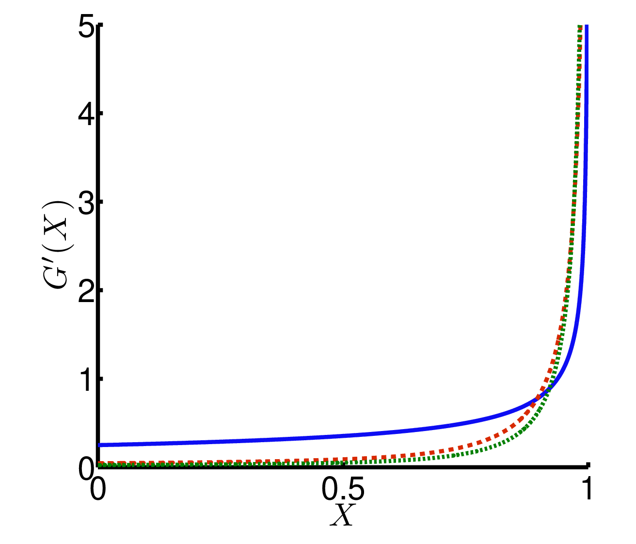
To show that also is convex we observe that is a monotonously increasing function of We evaluate numerically the derivative by plotting for a wide range of , cf. figure 4, and see explicitly its monotonicity. More generally, one can check whether or not is convex for any exponent . It can then be observed numerically (not shown) that is not convex for any .
So far we discussed the case of integer spin. For half-integer spin, the ideas mentioned before cannot be used. Then, the derivative of can be obtained via the numerical derivation of Based on numerics, we can make the same statements about the convexity of and as for the case of an integer spin.
References
- [1] Schwemmer C, Tóth G, Niggebaum A, Moroder T, Gross D, Gühne O and Weinfurter H 2014 Phys. Rev. Lett. 113 040503
- [2] Gao W B, Lu C Y, Yao X C, Xu P, Gühne O, Goebel A, Chen Y A, Peng C Z, Chen Z B and Pan J W 2010 Nat. Phys. 6 331–335
- [3] Leibfried D, Barrett M, Schaetz T, Britton J, Chiaverini J, Itano W, Jost J, Langer C and Wineland D 2004 Science 304 1476–1478
- [4] Huang Y F, Liu B H, Peng L, Li Y H, Li L, Li C F and Guo G C 2011 Nat. Commun. 2 546
- [5] Appel J, Windpassinger P J, Oblak D, Hoff U B, Kjærgaard N and Polzik E S 2009 PNAS 106 10960–10965
- [6] Sewell R J, Koschorreck M, Napolitano M, Dubost B, Behbood N and Mitchell M W 2012 Phys. Rev. Lett. 109 253605
- [7] Gross C, Zibold T, Nicklas E, Esteve J and Oberthaler M K 2010 Nature 464 1165–1169
- [8] Lücke B, Peise J, Vitagliano G, Arlt J, Santos L, Tóth G and Klempt C 2014 Phys. Rev. Lett. 112 155304
- [9] Hosten O, Engelsen N J, Krishnakumar R and Kasevich M A 2016 Nature 529 505–508
- [10] McConnell R, Zhang H, Hu J, Ćuk S and Vuletić V 2015 Nature 519 439–442
- [11] Haas F, Volz J, Gehr R, Reichel J and Esteve J 2014 Science 344 180–183
- [12] Horodecki R, Horodecki P, Horodecki M and Horodecki K 2009 Rev. Mod. Phys. 81 865–942
- [13] Gühne O and Tóth G 2009 Phys. Rep. 474 1–75
- [14] Pezzé L and Smerzi A 2009 Phys. Rev. Lett. 102 100401
- [15] Sørensen A, Duan L M, Cirac J and Zoller P 2001 Nature 409 63–66
- [16] Kitagawa M and Ueda M 1993 Phys. Rev. A 47 5138–5143
- [17] Wineland D J, Bollinger J J, Itano W M and Heinzen D J 1994 Phys. Rev. A 50 67–88
- [18] Sørensen A S and Mølmer K 2001 Phys. Rev. Lett. 86 4431–4434
- [19] Hyllus P, Pezzé L, Smerzi A and Tóth G 2012 Phys. Rev. A 86 012337
- [20] Hald J, Sørensen J L, Schori C and Polzik E S 1999 Phys. Rev. Lett. 83 1319–1322
- [21] Fernholz T, Krauter H, Jensen K, Sherson J F, Sørensen A S and Polzik E S 2008 Phys. Rev. Lett. 101 073601
- [22] Orzel C, Tuchman A K, Fenselau M L, Yasuda M and Kasevich M A 2001 Science 291 2386–2389
- [23] Riedel M F, Böhi P, Li Y, Hänsch T W, Sinatra A and Treutlein P 2010 Nature 464 1170–1173
- [24] Esteve J, Gross C, Weller A, Giovanazzi S and Oberthaler M 2008 Nature 455 1216–1219
- [25] Bohnet J G, Cox K C, Norcia M A, Weiner J M, Chen Z and Thompson J K 2014 Nat. Photon 8 731–736
- [26] Cox K C, Greve G P, Weiner J M and Thompson J K 2016 Phys. Rev. Lett. 116 093602
- [27] Meyer V, Rowe M A, Kielpinski D, Sackett C A, Itano W M, Monroe C and Wineland D J 2001 Phys. Rev. Lett. 86 5870–5873
- [28] Auccaise R, Araujo-Ferreira A G, Sarthour R S, Oliveira I S, Bonagamba T J and Roditi I 2015 Phys. Rev. Lett. 114 043604
- [29] Mitchell M W and Beduini F A 2014 New J. Phys. 16 073027
- [30] Tóth G, Knapp C, Gühne O and Briegel H J 2007 Phys. Rev. Lett. 99 250405
- [31] He Q Y, Peng S G, Drummond P D and Reid M D 2011 Phys. Rev. A 84 022107
- [32] Reis M S, Soriano S, dos Santos A M, Sales B C, Soares-Pinto D O and Brandão P 2012 Europhys. Lett. 100 50001
- [33] Behbood N, Ciurana F M, Colangelo G, Napolitano M, Tóth G, Sewell R J and Mitchell M W 2014 Phys. Rev. Lett. 113 093601
- [34] Vitagliano G, Apellaniz I, Egusquiza I L and Tóth G 2014 Phys. Rev. A 89 032307
- [35] Wieczorek W, Krischek R, Kiesel N, Michelberger P, Tóth G and Weinfurter H 2009 Phys. Rev. Lett. 103 020504
- [36] Prevedel R, Cronenberg G, Tame M S, Paternostro M, Walther P, Kim M S and Zeilinger A 2009 Phys. Rev. Lett. 103 020503
- [37] Lücke B, Scherer M, Kruse J, Pezzé L, Deuretzbacher F, Hyllus P, Peise J, Ertmer W, Arlt J, Santos L, Smerzi A and Klempt C 2011 Science 334 773–776
- [38] Hamley C, Gerving C, Hoang T, Bookjans E and Chapman M 2012 Nat. Phys. 8 305–308
- [39] Duan L M 2011 Phys. Rev. Lett. 107 180502
- [40] Zhang Z and Duan L M 2013 Phys. Rev. Lett. 111 180401
- [41] Hoang T M, Anquez M, Boguslawski M J, Bharath H M, Robbins B A and Chapman M S 2016 Proc. Natl. Acad. Sci. 113 9465
- [42] Gühne O, Tóth G and Briegel H J 2005 New J. Phys. 7 229
- [43] de Echaniz S R, Mitchell M W, Kubasik M, Koschorreck M, Crepaz H, Eschner J and Polzik E S 2005 J. Opt. B: Quantum and Semiclassical Opt. 7 S548
- [44] Hyllus P, Laskowski W, Krischek R, Schwemmer C, Wieczorek W, Weinfurter H, Pezzé L and Smerzi A 2012 Phys. Rev. A 85 022321
- [45] Tóth G 2012 Phys. Rev. A 85 022322
- [46] Zhang Z and Duan L M 2014 New J. Phys. 16 103037
- [47] Tóth G and Apellaniz I 2014 J. Phys. A: Math. Theor. 47 424006
- [48] Apellaniz I, Lücke B, Peise J, Klempt C and Tóth G 2015 New J. Phys. 17 083027
- [49] Apellaniz I, Kleinmann M, Gühne O and Tóth G (Preprint 1511.05203)
- [50] Vitagliano G, Hyllus P, Egusquiza I L and Tóth G 2011 Phys. Rev. Lett. 107 240502