跳到论文正文
W Papers独立论文阅读器 arXiv:1605.07098 论文正文 计算阅读时间 · 0%
引用这篇论文根据当前论文元数据生成,正式投稿前建议核对。


License: arXiv.org perpetual non-exclusive license
arXiv:1605.07098v1 [cs.IT] 23 May 2016

Free Deterministic Equivalents for the Analysis of MIMO Multiple Access Channel

An-An Lu    Xiqi Gao       Chengshan Xiao    Thanks: The work of A.-A.˜Lu and X.˜Q.˜Gao was supported in part by National Natural Science Foundation of China under Grants 61320106003, 61471113 and 61401095, the China High-Tech 863 Plan under Grant Grants 2015AA01A701 and 2014AA01A704, National Science and Technology Major Project of China under Grant 2014ZX03003006-003, and the Huawei Cooperation Project. The work of C.˜Xiao was supported in part by the U.S. National Science Foundation under Grants ECCS-1231848 and ECCS-1539316. Part of this work was carried out while An-An Lu was visiting Missouri University of Science and Technology, Rolla, MO. Part of the material in this paper was presented at the IEEE International Conference on Communications, London, U.K., June 2015. Thanks: A.-A.˜Lu and X.˜Q.˜Gao are with the National Mobile Communications Research Laboratory, Southeast University, Nanjing 210096, China (e-mail: aalu@seu.edu.cn, xqgao@seu.edu.cn). Thanks: C.˜Xiao is with the Department of Electrical and Computer Engineering, Missouri University of Science and Technology, Rolla, MO 65409, USA ( email: xiaoc@mst.edu). Thanks: Communicated by O.˜Simeone, Associate Editor for Communications. Thanks: Copyright ©˜2014 IEEE. Personal use of this material is permitted. However, permission to use this material for any other purposes must be obtained from the IEEE by sending a request to pubs-permissions@ieee.org.
Abstract

In this paper, a free deterministic equivalent is proposed for the capacity analysis of the multi-input multi-output (MIMO) multiple access channel (MAC) with a more general channel model compared to previous works. Specifically, a MIMO MAC with one base station (BS) equipped with several distributed antenna sets is considered. Each link between a user and a BS antenna set forms a jointly correlated Rician fading channel. The analysis is based on operator-valued free probability theory, which broadens the range of applicability of free probability techniques tremendously. By replacing independent Gaussian random matrices with operator-valued random variables satisfying certain operator-valued freeness relations, the free deterministic equivalent of the considered channel Gram matrix is obtained. The Shannon transform of the free deterministic equivalent is derived, which provides an approximate expression for the ergodic input-output mutual information of the channel. The sum-rate capacity achieving input covariance matrices are also derived based on the approximate ergodic input-output mutual information. The free deterministic equivalent results are easy to compute, and simulation results show that these approximations are numerically accurate and computationally efficient.

Index Terms: 
Operator-valued free probability, deterministic equivalent, massive multi-input multi-output (MIMO), multiple access channel (MAC).

I Introduction

For the development of next generation communication systems, massive multiple-input multiple-output (MIMO) technology has been widely investigated during the last few years [1, 2, 3, 4, 5, 6]. Massive MIMO systems provide huge capacity enhancement by employing hundreds of antennas at a base station (BS). The co-location of so many antennas on a single BS is a major challenge in realizing massive MIMO, whereas dividing the BS antennas into distributed antenna sets (ASs) provides an alternative solution [7]. In most massive MIMO literature, it is assumed that each user equipment (UE) is equipped with a single-antenna. Since multiple antenna UEs are already used in practical systems, it would be of both theoretical and practical interest to investigate the capacity of massive MIMO with distributed ASs and multiple antenna users.

In [8], Zhang et al. investigated the capacity of a MIMO multiple access channel (MAC) with distributed sets of correlated antennas. The results of [8] can be applied to a massive MIMO uplink with distributed ASs and multiple antenna UEs directly. The channel between a user and an AS in [8] is assumed to be a Kronecker correlated MIMO channel [9] with line-of-sight (LOS) components. In [10], Oestges concluded that the validity of the Kronecker model decreases as the array size increases. Thus, we consider in this paper a MIMO MAC with a more general channel model than that in [8]. More precisely, we consider also distributed ASs and multiple antenna UEs, but assume that each link between a user and an AS forms a jointly correlated Rician fading channel [11, 12]. If the BS antennas become co-located, then the considered channel model reduces to that in [13]. To the best of our knowledge, a capacity analysis for such MIMO MACs has not been addressed to date.

For the MIMO MAC under consideration, an exact capacity analysis is difficult and might be unsolvable when the number of antennas grows large. In this paper, we aim at deriving an approximate capacity expression. Deterministic equivalents [14], which have been addressed extensively, are successful methods to derive the approximate capacity for various MIMO channels. These deterministic equivalent approaches fall into four main categories: the Bai and Silverstein method[15, 16, 17], the Gaussian method[18, 19, 8], the replica method[20, 13] and free probability theory[21, 22].

The Bai and Silverstein method has been applied to various MIMO MACs. Couillet et al. [15] used it to investigate the capacity of a MIMO MAC with separately correlated channels. Combining it with the generalized Lindeberg principle [23], Wen et al. [17] derived the ergodic input-output mutual information of a MIMO MAC where the channel matrix consists of correlated non-Gaussian entries. In the Bai and Silverstein method, one needs to “guess” the deterministic equivalent of the Stieltjes transform. This limits its applicability since the deterministic equivalents of some involved models might be hard to “guess” [14]. By using an integration by parts formula and the Nash-Poincare inequality, the Gaussian method is able to derive directly the deterministic equivalents and can be applied to random matrices with involved correlations. It is particularly suited to random matrices with Gaussian entries. Combined with the Lindeberg principle, the Gaussian method can be used to treat random matrices with non-Gaussian entries as in [8].

The replica method developed in statistical physics [24] is a widely used approach in wireless communications. It has also been applied to the MIMO MAC. Wen et al. [13] used it to investigate the sum-rate of multiuser MIMO uplink channels with jointly correlated Rician fading. Free probability theory [25] provides a better way to understand the asymptotic behavior of large dimensional random matrices. It was first applied to wireless communications by Evans and Tse to investigate the multiuser wireless communication systems [26].

The Bai and Silverstein method and the Gaussian method are very flexible. Both of them have been used to handle deterministic equivalents for advanced Haar models [16, 27]. Although its validity has not yet been proved [14], the replica method is also a powerful tool. Meanwhile, the applicability of free probability theory is commonly considered very limited as it can be only applied to large random matrices with unitarily invariant properties, such as standard Gaussian matrices and Haar unitary matrices.

The domain of applicability of free probability techniques can be broadened tremendously by operator-valued free probability theory [28, 29], which is a more general version of free probability theory and allows one to deal with random matrices with correlated entries [21]. In [21], Far et al. first used operator-valued free probability theory in wireless communications to study slow-fading MIMO systems with nonseparable correlation. The results of [21] were then used by Pan et al. to study the approximate capacity of uplink network MIMO systems [30] and the asymptotic spectral efficiency of uplink MIMO-CDMA systems over arbitrarily spatially correlated Rayleigh fading channels [31]. Quaternionic free probability used in [32] by Müller and Cakmak can be seen as a particular kind of operator-valued free probability[33].

In [22], Speicher and Vargas provided the free deterministic equivalent method to derive the deterministic equivalents under the operator-valued free probability framework. A free deterministic equivalent of a random matrix is a non-commutative random variable or an operator-valued random variable, and the difference between the distribution of the latter and the expected distribution of the random matrix goes to zero in the large dimension limit. They viewed the considered random matrix as a polynomial in several matrices, and obtained its free deterministic equivalent by replacing the matrices with operator-valued random variables satisfying certain freeness relations. They observed that the Cauchy transform of the free deterministic equivalent is actually the solution to the iterative deterministic equivalent equation derived by the Bai and Silverstein method or the Gaussian method. Using the free deterministic equivalent approach, they recovered the deterministic equivalent results for the advanced Haar model from [34].

Motivated by the results from [22], we propose a free deterministic equivalent for the capacity analysis of the general channel model considered in this paper. The method of free deterministic equivalents provides a relatively formalized methodology to obtain the deterministic equivalent of the Cauchy transform. By replacing independent Gaussian matrices with random matrices that are composed of non-commutative random variables and satisfying certain operator-valued freeness relations, we obtain the free deterministic equivalent of the channel Gram matrix. The Cauchy transform of the free deterministic equivalent is easy to derive by using operator-valued free probability techniques, and is asymptotically the same as that of the channel Gram matrix. Then, we compute the approximate Shannon transform of the channel Gram matrix and the approximate ergodic input-output mutual information of the channel. Furthermore, we derive the sum-rate capacity achieving input covariance matrices based on the approximate ergodic input-output mutual information.

Our considered channel model reduces to that in [8] when the channel between a user and an AS is a Kronecker correlated MIMO channel, and to the channel model in [13] when there is one AS at the BS. In this paper, we will show that the results of [8] and [13] can be recovered by using the free deterministic equivalent method. Since many existing channel models are special cases of the channel models in [8] and [13], we will also be able to provide a new approach to derive the deterministic equivalent results for them.

The rest of this article is organized as follows. The preliminaries and problem formulation are presented in Section II. The main results are provided in Section III. Simulations are contained in Section IV. The conclusion is drawn in Section V. A tutorial on free probability theory and operator-valued free probability theory is presented in Appendix A, where the free deterministic equivalents used in this paper are also introduced and a rigorous mathematical justification of the free deterministic equivalents is provided. Proofs of Lemmas and Theorems are provided in Appendices B to G.

Notations: Throughout this paper, uppercase boldface letters and lowercase boldface letters are used for matrices and vectors, respectively. The superscripts (⋅)∗(\cdot)^{*}, (⋅)T(\cdot)^{T} and (⋅)H(\cdot)^{H} denote the conjugate, transpose and conjugate transpose operations, respectively. The notation 𝔼​{⋅}{\mathbb{E}}\{\cdot\} denotes the mathematical expectation operator. In some cases, where it is not clear from the context, we will employ subscripts to emphasize the definition. The notation g∘fg\circ f represents the composite function g⁡(f⁡(x))g(f(x)). We use 𝐀⊙𝐁\mathbf{A}\odot\mathbf{B} to denote the Hadamard product of two matrices 𝐀\mathbf{A} and 𝐁\mathbf{B} of the same dimensions. The N×NN\times N identity matrix is denoted by 𝐈N\mathbf{I}_{N}. The N×NN\times N and N×MN\times M zero matrices are denoted by 𝟎N\mathbf{0}_{N} and 𝟎N×M\mathbf{0}_{N\times M}. We use [𝐀]i​j[\mathbf{A}]_{ij} to denote the (i,j)(i,j)-th entry of the matrix 𝐀\mathbf{A}. The operators tr⁡(⋅){\rm{tr}}(\cdot) and det(⋅)\det(\cdot) represent the matrix trace and determinant, respectively. diag⁡(𝐱){\rm{diag}}(\mathbf{x}) denotes a diagonal matrix with 𝐱\mathbf{x} along its main diagonal. ℜ⁡(𝐖)\Re(\mathbf{W}) and ℑ⁡(𝐖)\Im(\mathbf{W}) denote 12​(𝐖+𝐖H)\frac{1}{2}(\mathbf{W}+\mathbf{W}^{H}) and 12​i​(𝐖−𝐖H)\frac{1}{2i}(\mathbf{W}-\mathbf{W}^{H}), respectively. 𝐃N​(ℂ)\mathbf{D}_{N}(\mathbb{C}) denotes the algebra of N×NN\times N diagonal matrices with elements in the complex field ℂ\mathbb{C}. Finally, we denote by 𝐌N​(ℂ)\mathbf{M}_{N}(\mathbb{C}) the algebra of N×NN\times N complex matrices and by 𝐌N×M​(ℂ)\mathbf{M}_{N\times M}(\mathbb{C}) the algebra of N×MN\times M complex matrices.

II Preliminaries and Problem Formulation

In this section, we first present the definitions of the Shannon transform and the Cauchy transform, and introduce the free deterministic equivalent method with a simple channel model, while our rigorous mathematical justification of the free deterministic equivalents is provided in Appendix A. Then, we present the general model of the MIMO MAC considered in this work, followed by the problem formulation.

II-A Shannon Transform and Cauchy Transform

Let 𝐇\mathbf{H} be an N×MN\times M random matrix and 𝐁N{\mathbf{B}_{N}} denote the Gram matrix 𝐇𝐇H\mathbf{H}\mathbf{H}^{H}. Let F𝐁N​(λ)F_{\mathbf{B}_{N}}(\lambda) denote the expected cumulative distribution of the eigenvalues of 𝐁N{\mathbf{B}_{N}}. The Shannon transform 𝒱𝐁N​(x)\mathcal{V}_{\mathbf{B}_{N}}(x) is defined as [35]

𝒱𝐁N​(x)=∫0∞log⁡(1+1x​λ)​d​F𝐁N​(λ).\mathcal{V}_{\mathbf{B}_{N}}(x)=\int_{0}^{\infty}\log(1+\frac{1}{x}\lambda)dF_{\mathbf{B}_{N}}(\lambda). (1)

Let μ\mu be a probability measure on ℝ\mathbb{R} and ℂ+\mathbb{C}^{+} denote the set

{z∈ℂ:ℑ⁡(z)>0}.\left\{z\in\mathbb{C}:\Im(z)>0\right\}.

The Cauchy transform Gμ​(z)G_{\mu}(z) for z∈ℂ+z\in\mathbb{C}^{+} is defined by [36]

Gμ​(z)=∫0∞1z−λ​𝑑μ​(λ).\displaystyle{G}_{\mu}(z)=\int_{0}^{\infty}\frac{1}{z-\lambda}d\mu(\lambda). (2)

Let G𝐁N​(z)G_{\mathbf{B}_{N}}(z) denote the Cauchy transform for F𝐁N​(λ)F_{\mathbf{B}_{N}}(\lambda). Then, we have G𝐁N​(z)=1N​𝔼​{tr⁡((z​𝐈N−𝐁N)−1)}.G_{\mathbf{B}_{N}}(z)=\frac{1}{N}{\mathbb{E}}\{{\rm{tr}}((z\mathbf{I}_{N}-\mathbf{B}_{N})^{-1})\}. The relation between the Cauchy transform G𝐁N​(z)G_{\mathbf{B}_{N}}(z) and the Shannon transform 𝒱𝐁N​(x)\mathcal{V}_{\mathbf{B}_{N}}(x) can be expressed as [35]

𝒱𝐁N​(x)=∫x+∞(1z+G𝐁N​(−z))​𝑑z.\mathcal{V}_{\mathbf{B}_{N}}(x)=\int_{x}^{+\infty}\left(\frac{1}{z}+G_{\mathbf{B}_{N}}(-z)\right)dz. (3)

Differentiating both sides of (3) with respect to xx, we obtain

d​𝒱𝐁N​(x)d​x=−x−1−G𝐁N​(−x).\frac{d\mathcal{V}_{\mathbf{B}_{N}}(x)}{dx}=-x^{-1}-G_{\mathbf{B}_{N}}(-x). (4)

Thus, if we are able to find a function whose derivative with respect to xx is −x−1−G𝐁N​(−x)-x^{-1}-G_{\mathbf{B}_{N}}(-x), then we can obtain 𝒱𝐁N​(x)\mathcal{V}_{\mathbf{B}_{N}}(x). In conclusion, if the Cauchy transform G𝐁N​(x)G_{\mathbf{B}_{N}}(x) is known, then the Shannon transform 𝒱𝐁N​(x)\mathcal{V}_{\mathbf{B}_{N}}(x) can be immediately obtained by applying (4).

II-B Free Deterministic Equivalent Method

In this subsection, we introduce the free deterministic equivalent method, which can be used to derive the approximation of G𝐁N​(z)G_{\mathbf{B}_{N}}(z). The associated definitions, such as that of free independence, circular elements, R-cyclic matrices and semicircular elements over 𝐃n​(ℂ)\mathbf{D}_{n}(\mathbb{C}), are provided in Appendix A-A.

The term free deterministic equivalent was coined by Speicher and Vargas in [22]. The considered random matrix in [22] was viewed as a polynomial in several deterministic matrices and several independent random matrices. The free deterministic equivalent of the considered random matrix was then obtained by replacing the matrices with operator-valued random variables satisfying certain freeness relations. Moreover, the difference between the Cauchy transform of the free deterministic equivalent and that of the considered random matrix goes to zero in the large dimension limit.

However, the method in [22] only showed how to obtain the free deterministic equivalents for the case where the random matrices are standard Gaussian matrices and Haar unitary matrices. A method similar to that in [22] was presented by Speicher in [37], which appeared earlier than [22]. The method in [37] showed that the random matrix with independent Gaussian entries having different variances can be replaced by the random matrix with free (semi)circular elements having different variances. But, it only considered a very simple case, and the replacement process had no rigorous mathematical proof. Moreover, the free deterministic equivalents were not mentioned in [37].

In this paper, we introduce in Appendix A-B the free deterministic equivalents for the case where all the matrices are square and have the same size, and the random matrices are Hermitian and composed of independent Gaussian entries with different variances. Similarly to [22], the free deterministic equivalent of a polynomial in matrices is defined. The replacement process used is that in [37]. Moreover, a rigorous mathematical justification of the free deterministic equivalents we introduce is also provided in Appendix A-B and Appendix A-C.

(z​𝒢𝓑𝑵𝒟N​(z2​𝐈N)𝟎𝟎z​𝒢𝓗H​𝓗𝒟M​(z2​𝐈M))\displaystyle\!\!\!\!\!\!\!\!\!\!\!\!\!\!\!\!\left(\begin{array}[]{cccccc}z\mathcal{G}_{\boldsymbol{\mathcal{B}_{N}}}^{\mathcal{D}_{N}}(z^{2}\mathbf{I}_{N})&\mathbf{0}\\ \mathbf{0}&z\mathcal{G}_{\boldsymbol{\mathcal{H}}^{H}\boldsymbol{\mathcal{H}}}^{\mathcal{D}_{M}}(z^{2}\mathbf{I}_{M})\\ \end{array}\right)
=E𝒟n​{(z​𝐈N−z​η𝒟N​(𝒢𝓗H​𝓗𝒟M​(z2​𝐈M))−𝐇¯−𝐇¯Hz​𝐈M−z​η𝒟M​(𝒢𝓑N𝒟N​(z2​𝐈N)))−1}\displaystyle=E_{\mathcal{D}_{n}}\left\{\left(\begin{array}[]{cccccc}z\mathbf{I}_{N}-z\eta_{\mathcal{D}_{N}}(\mathcal{G}_{\boldsymbol{\mathcal{H}}^{H}\boldsymbol{\mathcal{H}}}^{\mathcal{D}_{M}}(z^{2}\mathbf{I}_{M}))&-\overline{\mathbf{H}}\\ -\overline{\mathbf{H}}{}^{H}&z\mathbf{I}_{M}-z\eta_{\mathcal{D}_{M}}(\mathcal{G}_{\boldsymbol{\mathcal{B}}_{N}}^{\mathcal{D}_{N}}(z^{2}\mathbf{I}_{N}))\\ \end{array}\right)^{-1}\right\}


In [37], the deterministic equivalent results of [38] were rederived. But the description in [37] is not easy to follow. To show how the introduced free deterministic equivalents can be used to derive the approximation of the Cauchy transform G𝐁N​(z)G_{\mathbf{B}_{N}}(z), we use the channel model in [38] as a toy example and restate the method used in [37] as follows.

The channel matrix 𝐇\mathbf{H} in [38] consists of an N×MN\times M deterministic matrix 𝐇¯\overline{\mathbf{H}} and an N×MN\times M random matrix 𝐇~\widetilde{\mathbf{H}}, i.e., 𝐇=𝐇¯+𝐇~\mathbf{H}=\overline{\mathbf{H}}+\widetilde{\mathbf{H}}. The entries of 𝐇~\widetilde{\mathbf{H}} are independent zero mean complex Gaussian random variables with variances 𝔼⁡{[𝐇~]i​j​[𝐇~]i​j∗}=1N​σi​j2\mathbb{E}\{[\widetilde{\mathbf{H}}]_{ij}[\widetilde{\mathbf{H}}]_{ij}^{*}\}=\frac{1}{N}\sigma_{ij}^{2}.

Let nn denote N+MN+M, 𝒫\mathcal{P} denote the algebra of complex random variables and 𝐌n​(𝒫)\mathbf{M}_{n}(\mathcal{P}) denote the algebra of n×nn\times n complex random matrices. We define 𝔼𝒟n:𝐌n​(𝒫)→𝐃n​(ℂ)\mathbb{E}_{\mathcal{D}_{n}}:\mathbf{M}_{n}(\mathcal{P})\rightarrow\mathbf{D}_{n}(\mathbb{C}) by

𝔼𝒟n​{(X11X12⋯X1​nX21X22…X2​n⋮⋮⋱⋮Xn​1Xn​2…Xn​n)}\displaystyle\!\!\!\!\!\!\!\!\!\!\!\!{\mathbb{E}}_{\mathcal{D}_{n}}\left\{\left(\begin{array}[]{ccccc}X_{11}&X_{12}&\cdots&X_{1n}\\ X_{21}&X_{22}&\ldots&X_{2n}\\ \vdots&\vdots&\ddots&\vdots\\ X_{n1}&X_{n2}&\ldots&X_{nn}\\ \end{array}\right)\right\}
=(𝔼​{X11}0⋯00𝔼​{X22}⋯0⋮⋮⋱⋮00…𝔼​{Xn​n})\displaystyle=\left(\begin{array}[]{cccc}{\mathbb{E}}\{X_{11}\}&0&\cdots&0\\ 0&{\mathbb{E}}\{X_{22}\}&\cdots&0\\ \vdots&\vdots&\ddots&\vdots\\ 0&0&\ldots&{\mathbb{E}}\{X_{nn}\}\\ \end{array}\right)

where each Xi​jX_{ij} is a complex random variable. Hereafter, we use the notations ℳn:=𝐌n​(ℂ)\mathcal{M}_{n}:=\mathbf{M}_{n}(\mathbb{C}) and 𝒟n:=𝐃n​(ℂ)\mathcal{D}_{n}:=\mathbf{D}_{n}(\mathbb{C}) for brevity.

Let 𝐗\mathbf{X} be an n×nn\times n matrix defined by [21]

𝐗=(𝟎N𝐇𝐇H𝟎M).\displaystyle{\mathbf{X}}=\left(\begin{array}[]{cc}\mathbf{0}_{N}&{\mathbf{H}}\\ {\mathbf{H}}^{H}&\mathbf{0}_{M}\\ \end{array}\right).

The matrix 𝐗\mathbf{X} is even, i.e., all the odd moments of 𝐗\mathbf{X} are zeros, and

𝐗2=(𝐇𝐇H𝟎N×M𝟎M×N𝐇H​𝐇).\displaystyle{\mathbf{X}}^{2}=\left(\begin{array}[]{cc}{\mathbf{H}}{\mathbf{H}}^{H}&\mathbf{0}_{N\times M}\\ \mathbf{0}_{M\times N}&{\mathbf{H}}^{H}{\mathbf{H}}\\ \end{array}\right).

Let 𝚫n∈𝒟n\boldsymbol{\Delta}_{n}\in\mathcal{D}_{n} be a diagonal matrix with ℑ⁡(𝚫n)≻0\Im(\boldsymbol{\Delta}_{n})\succ 0. The 𝒟n\mathcal{D}_{n}-valued Cauchy transform 𝒢𝐗𝒟n​(𝚫n)\mathcal{G}_{\mathbf{X}}^{\mathcal{D}_{n}}(\boldsymbol{\Delta}_{n}) is given by

𝒢𝐗𝒟n​(𝚫n)=𝔼𝒟n​{(𝚫n−𝐗)−1}.\displaystyle\mathcal{G}_{\mathbf{X}}^{\mathcal{D}_{n}}(\boldsymbol{\Delta}_{n})={\mathbb{E}}_{\mathcal{D}_{n}}\{(\boldsymbol{\Delta}_{n}-\mathbf{X})^{-1}\}. (21)

When 𝚫n=z​𝐈n\boldsymbol{\Delta}_{n}=z\mathbf{I}_{n} and z∈ℂ+z\in\mathbb{C}^{+}, we have that

𝒢𝐗𝒟n​(z​𝐈n)\displaystyle\!\!\!\!\!\!\!\!\!\!\!\!\!\!\mathcal{G}_{\mathbf{X}}^{\mathcal{D}_{n}}(z\mathbf{I}_{n})
=𝔼𝒟n​{(z​𝐈n−𝐗)−1}\displaystyle\!\!\!\!\!\!\!\!\!\!={\mathbb{E}}_{\mathcal{D}_{n}}\!\!\left\{(z\mathbf{I}_{n}-\mathbf{X})^{-1}\right\}
=𝔼𝒟n​{(z​(z2​𝐈N−𝐇𝐇H)−1𝐇​(z2​𝐈M−𝐇H​𝐇)−1𝐇H​(z2​𝐈N−𝐇𝐇H)−1z​(z2​𝐈M−𝐇H​𝐇)−1)}\displaystyle\!\!\!\!\!\!\!\!\!\!={\mathbb{E}}_{\mathcal{D}_{n}}\!\!\left\{\!\!\left(\!\!\begin{array}[]{cc}\!\!z(z^{2}\mathbf{I}_{N}-\mathbf{H}\mathbf{H}^{H})^{-1}&\!\!{\mathbf{H}}(z^{2}\mathbf{I}_{M}-\mathbf{H}^{H}\mathbf{H})^{-1}\\ \!\!{\mathbf{H}}^{H}(z^{2}\mathbf{I}_{N}-\mathbf{H}\mathbf{H}^{H})^{-1}&\!\!z(z^{2}\mathbf{I}_{M}-\mathbf{H}^{H}\mathbf{H})^{-1}\\ \end{array}\right)\!\!\right\}
(25)

where the second equality is due to the block matrix inversion formula [39]. From (II-B) and (25), we obtain

𝒢𝐗𝒟n​(z​𝐈n)=z​𝒢𝐗2𝒟n​(z2​𝐈n)\mathcal{G}_{\mathbf{X}}^{\mathcal{D}_{n}}(z\mathbf{I}_{n})=z\mathcal{G}_{\mathbf{X}^{2}}^{\mathcal{D}_{n}}(z^{2}\mathbf{I}_{n}) (26)

for each z,z2∈ℂ+z,z^{2}\in\mathbb{C}^{+}. Furthermore, we write 𝒢𝐗2𝒟n​(z​𝐈n)\mathcal{G}_{\mathbf{X}^{2}}^{\mathcal{D}_{n}}(z\mathbf{I}_{n}) as

𝒢𝐗2𝒟n​(z​𝐈n)=(𝒢𝐁N𝒟N​(z​𝐈N)𝟎𝟎𝒢𝐇H​𝐇𝒟M​(z​𝐈M))\mathcal{G}_{\mathbf{X}^{2}}^{\mathcal{D}_{n}}(z\mathbf{I}_{n})=\left(\begin{array}[]{cccccc}\mathcal{G}_{\mathbf{B}_{N}}^{\mathcal{D}_{N}}(z\mathbf{I}_{N})&\mathbf{0}\\ \mathbf{0}&\mathcal{G}_{{\mathbf{H}}^{H}{\mathbf{H}}}^{\mathcal{D}_{M}}(z\mathbf{I}_{M})\\ \end{array}\right) (27)

where

𝒢𝐁N𝒟N​(z​𝐈N)=𝔼𝒟N​{(z​𝐈N−𝐁N)−1}\displaystyle\mathcal{G}_{\mathbf{B}_{N}}^{\mathcal{D}_{N}}(z\mathbf{I}_{N})={\mathbb{E}}_{\mathcal{D}_{N}}\{(z\mathbf{I}_{N}-\mathbf{B}_{N})^{-1}\}
𝒢𝐇H​𝐇𝒟M​(z​𝐈M)=𝔼𝒟M​{(z​𝐈M−𝐇H​𝐇)−1}.\displaystyle\mathcal{G}_{{\mathbf{H}}^{H}{\mathbf{H}}}^{\mathcal{D}_{M}}(z\mathbf{I}_{M})={\mathbb{E}}_{\mathcal{D}_{M}}\{(z\mathbf{I}_{M}-{\mathbf{H}}^{H}{\mathbf{H}})^{-1}\}.

Since G𝐁N​(z)=1N​tr​(𝒢𝐁N𝒟N​(z​𝐈N))G_{\mathbf{B}_{N}}(z)=\frac{1}{N}{\rm{tr}}(\mathcal{G}_{\mathbf{B}_{N}}^{\mathcal{D}_{N}}(z\mathbf{I}_{N})), we have related the calculation of G𝐁N​(z){G}_{\mathbf{B}_{N}}(z) with that of 𝒢𝐗𝒟n​(z​𝐈n)\mathcal{G}_{\mathbf{X}}^{\mathcal{D}_{n}}(z\mathbf{I}_{n}).

We define 𝐗¯\overline{\mathbf{X}} and 𝐗~\widetilde{\mathbf{X}} by

𝐗¯=(𝟎N𝐇¯𝐇¯H𝟎M)\displaystyle\overline{\mathbf{X}}=\left(\begin{array}[]{cc}\mathbf{0}_{N}&\overline{\mathbf{H}}\\ \overline{\mathbf{H}}{}^{H}&\mathbf{0}_{M}\\ \end{array}\right)

and

𝐗~=(𝟎N𝐇~𝐇~H𝟎M).\displaystyle\widetilde{\mathbf{X}}=\left(\begin{array}[]{cc}\mathbf{0}_{N}&\widetilde{\mathbf{H}}\\ \widetilde{\mathbf{H}}^{H}&\mathbf{0}_{M}\\ \end{array}\right).

Then, we have that 𝐗=𝐗¯+𝐗~\mathbf{X}=\overline{\mathbf{X}}+\widetilde{\mathbf{X}}.

The free deterministic equivalent of 𝐗\mathbf{X} is constructed as follows. Let 𝒜\mathcal{A} be a unital algebra, (𝒜,ϕ)(\mathcal{A},\phi) be a non-commutative probability space and 𝓗~\widetilde{\boldsymbol{\mathcal{H}}} denote an N×MN\times M matrix with entries from 𝒜\mathcal{A}. The entries [𝓗~]i​j∈𝒜[\widetilde{\boldsymbol{\mathcal{H}}}]_{ij}\in\mathcal{A} are freely independent centered circular elements with variances ϕ⁡([𝓗~]i​j​[𝓗~]i​j∗)=1N​σi​j2\phi([\widetilde{\boldsymbol{\mathcal{H}}}]_{ij}[\widetilde{\boldsymbol{\mathcal{H}}}]_{ij}^{*})=\frac{1}{N}\sigma_{ij}^{2}. Let 𝓗\boldsymbol{\mathcal{H}} denote 𝐇¯+𝓗~\overline{\mathbf{H}}+\widetilde{\boldsymbol{\mathcal{H}}}, 𝓧~\widetilde{\boldsymbol{\mathcal{X}}} denote

𝓧~=(𝟎𝓗~𝓗~H𝟎)\displaystyle\widetilde{\boldsymbol{\mathcal{X}}}=\left(\begin{array}[]{ccccc}\mathbf{0}&\widetilde{\boldsymbol{\mathcal{H}}}\\ \widetilde{\boldsymbol{\mathcal{H}}}^{H}&\mathbf{0}\\ \end{array}\right)

and 𝓧\boldsymbol{\mathcal{X}} denote

𝓧=(𝟎𝓗𝓗H𝟎).\displaystyle\boldsymbol{\mathcal{X}}=\left(\begin{array}[]{ccccc}\mathbf{0}&\boldsymbol{\mathcal{H}}\\ \boldsymbol{\mathcal{H}}^{H}&\mathbf{0}\\ \end{array}\right).

It follows that 𝓧=𝐗¯+𝓧~\boldsymbol{\mathcal{X}}=\overline{\mathbf{X}}+\widetilde{\boldsymbol{\mathcal{X}}}. The matrix 𝓧\boldsymbol{\mathcal{X}} is the free deterministic equivalent of 𝐗\mathbf{X}.

We define E𝒟n:𝐌n​(𝒜)→𝒟nE_{\mathcal{D}_{n}}:\mathbf{M}_{n}(\mathcal{A})\rightarrow\mathcal{D}_{n} by

E𝒟n​{(x11x12⋯x1​nx21x22…x2​n⋮⋮⋱⋮xn​1xn​2…xn​n)}\displaystyle\!\!\!\!\!\!\!\!\!\!\!\!E_{\mathcal{D}_{n}}\left\{\left(\begin{array}[]{ccccc}x_{11}&x_{12}&\cdots&x_{1n}\\ x_{21}&x_{22}&\ldots&x_{2n}\\ \vdots&\vdots&\ddots&\vdots\\ x_{n1}&x_{n2}&\ldots&x_{nn}\\ \end{array}\right)\right\}
=(ϕ⁡(x11)0⋯00ϕ⁡(x22)⋯0⋮⋮⋱⋮00…ϕ⁡(xn​n))\displaystyle=\left(\begin{array}[]{cccc}\phi(x_{11})&0&\cdots&0\\ 0&\phi(x_{22})&\cdots&0\\ \vdots&\vdots&\ddots&\vdots\\ 0&0&\ldots&\phi(x_{nn})\\ \end{array}\right)

where each xi​jx_{ij} is a non-commutative random variable from (𝒜,ϕ)(\mathcal{A},\phi). Then, (𝐌n​(𝒜),E𝒟n)(\mathbf{M}_{n}(\mathcal{A}),E_{\mathcal{D}_{n}}) is a 𝒟n\mathcal{D}_{n}-valued probability space.

From the discussion of the free deterministic equivalents provided in Appendix A-B, we have that 𝒢𝓧𝒟n​(z​𝐈n)\mathcal{G}^{\mathcal{D}_{n}}_{\boldsymbol{\mathcal{X}}}(z\mathbf{I}_{n}) and 𝒢𝐗𝒟n​(z​𝐈n)\mathcal{G}^{\mathcal{D}_{n}}_{\mathbf{X}}(z\mathbf{I}_{n}) are asymptotically the same. Let 𝓑N\boldsymbol{\mathcal{B}}_{N} denote 𝓗​𝓗H\boldsymbol{\mathcal{H}}\boldsymbol{\mathcal{H}}^{H}. The relation between 𝒢𝓧𝒟n​(z​𝐈n)\mathcal{G}_{\boldsymbol{\mathcal{X}}}^{\mathcal{D}_{n}}(z\mathbf{I}_{n}) and 𝒢𝓑N𝒟N​(z​𝐈N)\mathcal{G}_{\boldsymbol{\mathcal{B}}_{N}}^{\mathcal{D}_{N}}(z\mathbf{I}_{N}) is the same as that between 𝒢𝐗𝒟n​(z​𝐈n)\mathcal{G}_{\mathbf{X}}^{\mathcal{D}_{n}}(z\mathbf{I}_{n}) and 𝒢𝐁N𝒟N​(z​𝐈N)\mathcal{G}_{\mathbf{B}_{N}}^{\mathcal{D}_{N}}(z\mathbf{I}_{N}). Thus, we also have that 𝒢𝓑N𝒟N​(z​𝐈N)\mathcal{G}_{\boldsymbol{\mathcal{B}}_{N}}^{\mathcal{D}_{N}}(z\mathbf{I}_{N}) and 𝒢𝐁N𝒟N​(z​𝐈N)\mathcal{G}_{\mathbf{B}_{N}}^{\mathcal{D}_{N}}(z\mathbf{I}_{N}) are asymptotically the same and G𝓑N​(z)G_{\boldsymbol{\mathcal{B}}_{N}}(z) is the deterministic equivalent of G𝐁N​(z)G_{\mathbf{B}_{N}}(z). For convenience, we also call 𝓑N\boldsymbol{\mathcal{B}}_{N} the free deterministic equivalent of 𝐁N\mathbf{B}_{N}. In the following, we derive the Cauchy transform G𝓑N​(z)G_{\boldsymbol{\mathcal{B}}_{N}}(z) by using operator-valued free probability techniques.

Since its elements on and above the diagonal are freely independent, we have that 𝓧~\widetilde{\boldsymbol{\mathcal{X}}} is an R-cyclic matrix. From Theorem 8.2 of [40], we then have that 𝐗¯\overline{\boldsymbol{\mathbf{X}}} and 𝓧~\widetilde{\boldsymbol{\mathcal{X}}} are free over 𝒟n\mathcal{D}_{n}. The 𝒟n\mathcal{D}_{n}-valued Cauchy transform of the sum of two 𝒟n\mathcal{D}_{n}-valued free random variables is given by (143) in Appendix A-A. Applying (143), we have that

𝒢𝓧𝒟n​(z​𝐈n)\displaystyle\!\!\!\!\mathcal{G}_{\boldsymbol{\mathcal{X}}}^{\mathcal{D}_{n}}(z\mathbf{I}_{n})\!\!\!\! =\displaystyle= 𝒢𝐗¯𝒟n​(z​𝐈n−ℛ𝓧~𝒟n​(𝒢𝓧𝒟n​(z​𝐈n)))\displaystyle\!\!\!\!\mathcal{G}_{\overline{\boldsymbol{\mathbf{X}}}}^{\mathcal{D}_{n}}\!\!\left(z\mathbf{I}_{n}-\mathcal{R}_{\widetilde{\boldsymbol{\mathcal{X}}}}^{\mathcal{D}_{n}}\!\!\left(\mathcal{G}_{\boldsymbol{\mathcal{X}}}^{\mathcal{D}_{n}}(z\mathbf{I}_{n})\right)\right) (50)
=\displaystyle= E𝒟n​{(z​𝐈n−ℛ𝓧~𝒟n​(𝒢𝓧𝒟n​(z​𝐈n))−𝐗¯)−1}\displaystyle\!\!\!\!E_{\mathcal{D}_{n}}\!\!\left\{\!\!\left(z\mathbf{I}_{n}-\mathcal{R}_{\widetilde{\boldsymbol{\mathcal{X}}}}^{\mathcal{D}_{n}}\!\!\left(\mathcal{G}_{\boldsymbol{\mathcal{X}}}^{\mathcal{D}_{n}}(z\mathbf{I}_{n})\right)-\overline{\boldsymbol{\mathbf{X}}}\right)^{-1}\!\!\right\}

where ℛ𝓧~𝒟n\mathcal{R}_{\widetilde{\boldsymbol{\mathcal{X}}}}^{\mathcal{D}_{n}} is the 𝒟n\mathcal{D}_{n}-valued R-transform of 𝓧\boldsymbol{\mathcal{X}}.

Let η𝒟n​(𝐂)\eta_{\mathcal{D}_{n}}(\mathbf{C}) denote E𝒟n​{𝓧~​𝐂​𝓧~}E_{\mathcal{D}_{n}}\{\widetilde{\boldsymbol{\mathcal{X}}}\mathbf{C}\widetilde{\boldsymbol{\mathcal{X}}}\}, where 𝐂∈𝒟n\mathbf{C}\in\mathcal{D}_{n}. From Theorem 7.2 of [40], we obtain that 𝓧~\widetilde{\boldsymbol{\mathcal{X}}} is semicircular over 𝒟n\mathcal{D}_{n}, and thus its 𝒟n\mathcal{D}_{n}-valued R-transform is given by

ℛ𝓧~𝒟n​(𝐂)=η𝒟n​(𝐂).\mathcal{R}_{\widetilde{\boldsymbol{\mathcal{X}}}}^{\mathcal{D}_{n}}(\mathbf{C})=\eta_{\mathcal{D}_{n}}(\mathbf{C}). (51)

From (50) and the counterparts of (26) and (27) for 𝒢𝓧𝒟n​(z​𝐈n)\mathcal{G}_{\boldsymbol{\mathcal{X}}}^{\mathcal{D}_{n}}(z\mathbf{I}_{n}) and 𝒢𝓧2𝒟n​(z​𝐈n)\mathcal{G}_{\boldsymbol{\mathcal{X}}^{2}}^{\mathcal{D}_{n}}(z\mathbf{I}_{n}), we obtain equation (II-B) at the top of this page.

z𝒢𝓑N𝒟N(z𝐈N)=E𝒟N{(𝐈N−η𝒟N(𝒢𝓗H​𝓗𝒟M(z𝐈M))−𝐇¯(z𝐈M−zη𝒟M(𝒢𝓑N𝒟N(z𝐈N)))−1𝐇¯)H−1}\displaystyle\!\!\!\!z\mathcal{G}_{\boldsymbol{\mathcal{B}}_{N}}^{\mathcal{D}_{N}}(z\mathbf{I}_{N})=E_{\mathcal{D}_{N}}\left\{\left(\mathbf{I}_{N}-\eta_{\mathcal{D}_{N}}(\mathcal{G}_{\boldsymbol{\mathcal{H}}^{H}\boldsymbol{\mathcal{H}}}^{\mathcal{D}_{M}}(z\mathbf{I}_{M}))-\overline{\mathbf{H}}\left(z\mathbf{I}_{M}-z\eta_{\mathcal{D}_{M}}(\mathcal{G}_{\boldsymbol{\mathcal{B}}_{N}}^{\mathcal{D}_{N}}(z\mathbf{I}_{N}))\right)^{-1}\overline{\mathbf{H}}{}^{H}\right)^{-1}\right\} (20)
z𝒢𝓗H​𝓗𝒟M(z𝐈M)=E𝒟M{(𝐈M−η𝒟M(𝒢𝓑N𝒟N(z𝐈N))−𝐇¯(z𝐈N−zη𝒟N(𝒢𝓗H​𝓗𝒟M(z𝐈M)))−1H𝐇¯)−1}\displaystyle\!\!\!\!z\mathcal{G}_{\boldsymbol{\mathcal{H}}^{H}\boldsymbol{\mathcal{H}}}^{\mathcal{D}_{M}}(z\mathbf{I}_{M})=E_{\mathcal{D}_{M}}\left\{\left(\mathbf{I}_{M}-\eta_{\mathcal{D}_{M}}(\mathcal{G}_{\boldsymbol{\mathcal{B}}_{N}}^{\mathcal{D}_{N}}(z\mathbf{I}_{N}))-\overline{\mathbf{H}}{}^{H}\left(z\mathbf{I}_{N}-z\eta_{\mathcal{D}_{N}}(\mathcal{G}_{\boldsymbol{\mathcal{H}}^{H}\boldsymbol{\mathcal{H}}}^{\mathcal{D}_{M}}(z\mathbf{I}_{M}))\right)^{-1}\overline{\mathbf{H}}\right)^{-1}\right\} (21)


Furthermore, we obtain equations (20) and (21) at the top of the following page, where

η𝒟N(𝐂1)=E𝒟N{𝓗~𝐂1𝓗~}H,𝐂1∈𝒟M\displaystyle\eta_{\mathcal{D}_{N}}(\mathbf{C}_{1})=E_{\mathcal{D}_{N}}\{\widetilde{\boldsymbol{\mathcal{H}}}\mathbf{C}_{1}\widetilde{\boldsymbol{\mathcal{H}}}{}^{H}\},\mathbf{C}_{1}\in\mathcal{D}_{M}
η𝒟M​(𝐂2)=E𝒟M​{𝓗~​𝐂2H​𝓗~},𝐂2∈𝒟N.\displaystyle\eta_{\mathcal{D}_{M}}(\mathbf{C}_{2})=E_{\mathcal{D}_{M}}\{\widetilde{\boldsymbol{\mathcal{H}}}{}^{H}\mathbf{C}_{2}\widetilde{\boldsymbol{\mathcal{H}}}\},\mathbf{C}_{2}\in\mathcal{D}_{N}.

Equations (20) and (21) are equivalent to the ones provided by Theorem 2.4 of [38]. Finally, the Cauchy transform G𝓑N​(z)G_{\boldsymbol{\mathcal{B}}_{N}}(z) is obtained by G𝓑N​(z)=1N​tr​(𝒢𝓑N𝒟N​(z​𝐈N))G_{\boldsymbol{\mathcal{B}}_{N}}(z)=\frac{1}{N}{\rm{tr}}(\mathcal{G}_{\boldsymbol{\mathcal{B}}_{N}}^{\mathcal{D}_{N}}(z\mathbf{I}_{N})).

In conclusion, the free deterministic equivalent method provides a way to derive the approximation of the Cauchy transform G𝐁N​(z)G_{\mathbf{B}_{N}}(z). The fundamental step is to construct the free deterministic equivalent 𝓑N\boldsymbol{\mathcal{B}}_{N} of 𝐁N\mathbf{B}_{N}. After the construction, the Cauchy transform G𝓑N​(z)G_{\boldsymbol{\mathcal{B}}_{N}}(z) can be derived by using operator-valued free probability techniques. Moreover, G𝓑N​(z)G_{\boldsymbol{\mathcal{B}}_{N}}(z) is the deterministic equivalent of G𝐁N​(z)G_{\mathbf{B}_{N}}(z).

II-C General Channel Model of MIMO MAC

We consider a frequency-flat fading MIMO MAC channel with one BS and KK UEs. The BS antennas are divided into LL distributed ASs. The ll-th AS is equipped with NlN_{l} antennas. The kk-th UE is equipped with MkM_{k} antennas. Furthermore, we assume ∑l=1LNl=N\sum\nolimits_{l=1}^{L}N_{l}=N and ∑k=1KMk=M\sum\nolimits_{k=1}^{K}M_{k}=M. Let 𝐱k\mathbf{x}_{k} denote the Mk×1M_{k}\times 1 transmitted vector of the kk-th UE. The covariance matrices of 𝐱k\mathbf{x}_{k} are given by

𝔼⁡{𝐱k​𝐱k′H}={PkMk​𝐐k,if​k=k′𝟎,otherwise{\mathbb{E}}\{\mathbf{x}_{k}\mathbf{x}_{k^{\prime}}^{H}\}=\left\{\begin{array}[]{cc}\frac{P_{k}}{M_{k}}\mathbf{Q}_{k},&{\rm if}~k=k^{\prime}\\ \mathbf{0},&~~{\rm otherwise}\end{array}\right. (22)

where PkP_{k} is the total transmitted power of the kk-th UE, and 𝐐k\mathbf{Q}_{k} is an Mk×MkM_{k}\times M_{k} positive semidefinite matrix with the constraint tr⁡(𝐐k)≤Mk{\rm{tr}}(\mathbf{Q}_{k})\leq M_{k}. The received signal 𝐲\mathbf{y} for a single symbol interval can be written as

𝐲=∑k=1K𝐇k​𝐱k+𝐳\mathbf{y}=\sum\limits_{k=1}^{K}\mathbf{H}_{k}\mathbf{x}_{k}+\mathbf{z} (23)

where 𝐇k\mathbf{H}_{k} is the N×MkN\times M_{k} channel matrix between the BS and the kk-th UE, and 𝐳\mathbf{z} is a complex Gaussian noise vector distributed as 𝒞​𝒩​(0,σz2​𝐈N)\mathcal{CN}(0,\sigma_{z}^{2}\mathbf{I}_{N}). The channel matrix 𝐇k\mathbf{H}_{k} is normalized as

𝔼⁡{tr⁡(𝐇k​𝐇kH)}=N​MkM.\mathbb{E}\{{\rm{tr}}(\mathbf{H}_{k}\mathbf{H}_{k}^{H})\}=\frac{NM_{k}}{M}. (24)

Furthermore, 𝐇k\mathbf{H}_{k} has the following structure

𝐇k=𝐇¯k+𝐇~k\mathbf{H}_{k}=\overline{\mathbf{H}}_{k}+\widetilde{\mathbf{H}}_{k} (25)

where 𝐇¯k\overline{\mathbf{H}}_{k} and 𝐇~k\widetilde{\mathbf{H}}_{k} are defined by

𝐇¯k=(𝐇¯𝐇¯T1​k⋯T2​k𝐇¯)TL​kT\displaystyle\overline{\mathbf{H}}_{k}=\left(\vphantom{\widetilde{\mathbf{H}}}\overline{\mathbf{H}}{}_{1k}^{T}~\overline{\mathbf{H}}{}_{2k}^{T}~\cdots~\overline{\mathbf{H}}{}_{Lk}^{T}\right)^{T} (26)
𝐇~k=(𝐇~1​kT𝐇~2​kT⋯𝐇~L​kT)T.\displaystyle\widetilde{\mathbf{H}}_{k}=\left(\widetilde{\mathbf{H}}_{1k}^{T}~\widetilde{\mathbf{H}}_{2k}^{T}~\cdots~\widetilde{\mathbf{H}}_{Lk}^{T}\right)^{T}. (27)

Each 𝐇¯l​k\overline{\mathbf{H}}_{lk} is an Nl×MkN_{l}\times M_{k} deterministic matrix, and each 𝐇~l​k\widetilde{\mathbf{H}}_{lk} is a jointly correlated channel matrix defined by [11, 12]

𝐇~l​k=𝐔l​k​(𝐌l​k⊙𝐖l​k)​𝐕l​kH\widetilde{\mathbf{H}}_{lk}=\mathbf{U}_{lk}(\mathbf{M}_{lk}\odot{\mathbf{W}}_{lk})\mathbf{V}_{lk}^{H} (28)

where 𝐔l​k\mathbf{U}_{lk} and 𝐕l​k\mathbf{V}_{lk} are deterministic unitary matrices, 𝐌l​k\mathbf{M}_{lk} is an Nl×MkN_{l}\times M_{k} deterministic matrix with nonnegative elements, and 𝐖l​k\mathbf{W}_{lk} is a complex Gaussian random matrix with independent and identically distributed (i.i.d.), zero mean and unit variance entries. The jointly correlated channel model not only accounts for the correlation at both link ends, but also characterizes their mutual dependence. It provides a more adequate model for realistic massive MIMO channels since the validity of the widely used Kronecker model decreases as the number of antennas increases. Furthermore, the justification of using the jointly correlated channel model for massive MIMO channels has been provided in [41, 42, 43]. We assume that the channel matrices of different links are independent in this paper, i.e., when k≠mk\neq m or j≠nj\neq n, we have that

𝔼⁡{𝐇~k​j​𝐂j​n​𝐇~m​nH}=𝟎Nk×Nm\displaystyle{\mathbb{E}}\left\{\widetilde{\mathbf{H}}_{kj}\mathbf{C}_{jn}\widetilde{\mathbf{H}}_{mn}^{H}\right\}=\mathbf{0}_{N_{k}\times N_{m}} (29)
𝔼⁡{𝐇~k​jH​𝐂~k​m​𝐇~m​n}=𝟎Mj×Mn\displaystyle{\mathbb{E}}\left\{\widetilde{\mathbf{H}}_{kj}^{H}{\widetilde{\mathbf{C}}}_{km}\widetilde{\mathbf{H}}_{mn}\right\}=\mathbf{0}_{M_{j}\times M_{n}} (30)

where 𝐂j​n∈𝐌Mj×Mn​(ℂ)\mathbf{C}_{jn}\in\mathbf{M}_{M_{j}\times M_{n}}(\mathbb{C}) and 𝐂~k​m∈𝐌Nk×Nm​(ℂ)\widetilde{\mathbf{C}}_{km}\in\mathbf{M}_{N_{k}\times N_{m}}(\mathbb{C}). Let 𝐖~l​k\widetilde{\mathbf{W}}_{lk} denote 𝐌l​k⊙𝐖l​k\mathbf{M}_{lk}\odot{\mathbf{W}}_{lk}. We define 𝐆l​k\mathbf{G}_{lk} as 𝐆l​k=𝐌l​k⊙𝐌l​k\mathbf{G}_{lk}=\mathbf{M}_{lk}\odot\mathbf{M}_{lk}. The parameterized one-sided correlation matrix η~k​(𝐂k){\tilde{\eta}}_{k}(\mathbf{C}_{k}) is given by

η~k​(𝐂k)=\displaystyle{\tilde{\eta}}_{k}(\mathbf{C}_{k})= 𝔼⁡{𝐇~k​𝐂k​𝐇~kH}\displaystyle{\mathbb{E}}\left\{\widetilde{\mathbf{H}}_{k}\mathbf{C}_{k}\widetilde{\mathbf{H}}_{k}^{H}\right\}
=\displaystyle= diag⁡(𝐔1​k​𝚷~1​k​(𝐂k)​𝐔1​kH,𝐔2​k​𝚷~2​k​(𝐂k)​𝐔2​kHCLOSE,\displaystyle{\rm{diag}}\left(\mathbf{U}_{1k}\widetilde{\mathbf{\Pi}}_{1k}(\mathbf{C}_{k})\mathbf{U}_{1k}^{H},\mathbf{U}_{2k}\widetilde{\mathbf{\Pi}}_{2k}(\mathbf{C}_{k})\mathbf{U}_{2k}^{H},\right. (31)
OPEN⋯,𝐔L​k​𝚷~L​k​(𝐂k)​𝐔L​kH)\displaystyle~~~~~~~~~~~~~~~~~~~~\left.\cdots,\mathbf{U}_{Lk}\widetilde{\mathbf{\Pi}}_{Lk}(\mathbf{C}_{k})\mathbf{U}_{Lk}^{H}\right)

where 𝐂k∈ℳMk\mathbf{C}_{k}\in\mathcal{M}_{M_{k}}, and 𝚷~l​k​(𝐂k)\widetilde{\mathbf{\Pi}}_{lk}(\mathbf{C}_{k}) is an Nl×NlN_{l}\times N_{l} diagonal matrix valued function with the diagonal entries obtained by

[𝚷~l​k​(𝐂k)]i​i=∑j=1Mk[𝐆l​k]i​j​[𝐕l​kH​𝐂k​𝐕l​k]j​j.\left[\widetilde{\mathbf{\Pi}}_{lk}(\mathbf{C}_{k})\right]_{ii}=\sum\limits_{j=1}^{M_{k}}\left[{\mathbf{G}}_{lk}\right]_{ij}\left[\mathbf{V}_{lk}^{H}\mathbf{C}_{k}\mathbf{V}_{lk}\right]_{jj}. (32)

Similarly, the other parameterized one-sided correlation matrix ηk​(𝐂~){\eta}_{k}(\widetilde{\mathbf{C}}) is expressed as

ηk​(𝐂~)=𝔼⁡{𝐇~kH​𝐂~​𝐇~k}=∑l=1L𝐕l​k​𝚷l​k​(⟨𝐂~⟩l)​𝐕l​kH{\eta}_{k}(\widetilde{\mathbf{C}})={\mathbb{E}}\left\{\widetilde{\mathbf{H}}_{k}^{H}{\widetilde{\mathbf{C}}}\widetilde{\mathbf{H}}_{k}\right\}=\sum\limits_{l=1}^{L}\mathbf{V}_{lk}{\mathbf{\Pi}}_{lk}(\langle{\widetilde{\mathbf{C}}}\rangle_{l})\mathbf{V}_{lk}^{H} (33)

where 𝐂~∈ℳN\widetilde{\mathbf{C}}\in\mathcal{M}_{N}, the notation ⟨𝐂~⟩l\langle{\widetilde{\mathbf{C}}}\rangle_{l} denotes the Nl×NlN_{l}\times N_{l} diagonal block of 𝐂~\widetilde{\mathbf{C}}, i.e., the submatrix of 𝐂~{\widetilde{\mathbf{C}}} obtained by extracting the entries of the rows and columns with indices from ∑i=1l−1Ni+1\sum\nolimits_{i=1}^{l-1}N_{i}+1 to ∑i=1lNi\sum\nolimits_{i=1}^{l}N_{i}, and 𝚷l​k​(⟨𝐂~⟩l){\mathbf{\Pi}}_{lk}(\langle{\widetilde{\mathbf{C}}}\rangle_{l}) is an Mk×MkM_{k}\times M_{k} diagonal matrix valued function with the diagonal entries computed by

[𝚷l​k​(⟨𝐂~⟩l)]i​i=∑j=1Nl[𝐆l​k]j​i​[𝐔l​kH​⟨𝐂~⟩l​𝐔l​k]j​j.\left[{\mathbf{\Pi}}_{lk}(\langle{\widetilde{\mathbf{C}}}\rangle_{l})\right]_{ii}=\sum\limits_{j=1}^{N_{l}}\left[{\mathbf{G}}_{lk}\right]_{ji}\left[\mathbf{U}_{lk}^{H}\langle{\widetilde{\mathbf{C}}}\rangle_{l}\mathbf{U}_{lk}\right]_{jj}. (34)

The channel model described above is suitable for describing cellular systems employing cooperative multipoint (CoMP) processing [44], and also conforms with the framework of cloud radio access networks (C-RANs) [45]. Moreover, it embraces many existing channel models as special cases. When L=1L=1, the MIMO MAC in [13] is described. Let 𝐉l​k\mathbf{J}_{lk} be an Nl×MkN_{l}\times M_{k} matrix of all 11s, 𝚲r,l​k\boldsymbol{\Lambda}_{r,lk} be an Nl×NlN_{l}\times N_{l} diagonal matrix with positive entries and 𝚲t,l​k\boldsymbol{\Lambda}_{t,lk} be an Mk×MkM_{k}\times M_{k} diagonal matrix with positive entries. Set 𝐌l​k=𝚲r,l​k1/2​𝐉l​k​𝚲t,l​k1/2\mathbf{M}_{lk}=\boldsymbol{\Lambda}_{r,lk}^{1/2}\mathbf{J}_{lk}\boldsymbol{\Lambda}_{t,lk}^{1/2}. Then, we obtain 𝐇~l​k=𝐔l​k​(𝚲r,l​k1/2​𝐉l​k​𝚲t,l​k1/2⊙𝐖l​k)​𝐕l​kH=𝐔l​k​𝚲r,l​k1/2​(𝐉l​k⊙𝐖l​k)​𝚲t,l​k1/2​𝐕l​kH\widetilde{\mathbf{H}}_{lk}=\mathbf{U}_{lk}(\boldsymbol{\Lambda}_{r,lk}^{1/2}\mathbf{J}_{lk}\boldsymbol{\Lambda}_{t,lk}^{1/2}\odot{\mathbf{W}}_{lk})\mathbf{V}_{lk}^{H}=\mathbf{U}_{lk}\boldsymbol{\Lambda}_{r,lk}^{1/2}(\mathbf{J}_{lk}\odot{\mathbf{W}}_{lk})\boldsymbol{\Lambda}_{t,lk}^{1/2}\mathbf{V}_{lk}^{H} [46]. Thus, each 𝐇~l​k\widetilde{\mathbf{H}}_{lk} reduces to the Kronecker model, and the considered channel model reduces to that in [8]. Many channel models are already included in the channel models of [8] and [13]. See the references for more details.

II-D Problem Formulation

Let 𝐇\mathbf{H} denote [𝐇1𝐇2⋯𝐇K][\mathbf{H}_{1}~\mathbf{H}_{2}~\cdots~\mathbf{H}_{K}]. In this paper, we are interested in computing the ergodic input-output mutual information of the channel 𝐇\mathbf{H} and deriving the sum-rate capacity achieving input covariance matrices. In particular, we consider the large-system regime where LL and KK are fixed but NlN_{l} and MkM_{k} go to infinity with ratios MkNl=βl​k\frac{M_{k}}{N_{l}}=\beta_{lk} such that

0<min⁡lim infNl,k⁡βl​k<max⁡lim supNl,k⁡βl​k<∞.0<\min\limits_{l,k}\liminf\limits_{N}\beta_{lk}<\max\limits_{l,k}\limsup\limits_{N}\beta_{lk}<\infty. (35)

We first consider the problem of computing the ergodic input-output mutual information. For simplicity, we assume PkMk​𝐐k=𝐈Mk\frac{P_{k}}{M_{k}}\mathbf{Q}_{k}=\mathbf{I}_{M_{k}}. The results for general precoders can then be obtained by replacing 𝐇k\mathbf{H}_{k} with PkMk​𝐇k​𝐐k12\sqrt{\frac{P_{k}}{M_{k}}}\mathbf{H}_{k}\mathbf{Q}_{k}^{\frac{1}{2}}. Let ℐ𝐁N​(σz2)\mathcal{I}_{\mathbf{B}_{N}}(\sigma_{z}^{2}) denote the ergodic input-output mutual information of the channel 𝐇{\mathbf{H}} and 𝐁N\mathbf{B}_{N} denote the channel Gram matrix 𝐇𝐇H{\mathbf{H}}{\mathbf{H}}^{H}. Under the assumption that the transmitted vector is a Gaussian random vector having an identity covariance matrix and the receiver at the BS has perfect channel state information (CSI), ℐ𝐁N​(σz2)\mathcal{I}_{\mathbf{B}_{N}}(\sigma_{z}^{2}) is given by [47]

ℐ𝐁N(σz2)=𝔼{logdet(𝐈N+1σz2𝐁N)}.{\mathcal{I}_{\mathbf{B}_{N}}(\sigma_{z}^{2})}={\mathbb{E}}\left\{\log\det(\mathbf{I}_{N}+\frac{1}{\sigma_{z}^{2}}\mathbf{B}_{N})\right\}. (36)

Furthermore, we have ℐ𝐁N​(σz2)=N​𝒱𝐁N​(σz2)\mathcal{I}_{\mathbf{B}_{N}}(\sigma_{z}^{2})=N\mathcal{V}_{\mathbf{B}_{N}}(\sigma_{z}^{2}). For the considered channel model, an exact expression of ℐ𝐁N​(σz2)\mathcal{I}_{\mathbf{B}_{N}}(\sigma_{z}^{2}) is intractable. Instead, our goal is to find an approximation of ℐ𝐁N​(σz2)\mathcal{I}_{\mathbf{B}_{N}}(\sigma_{z}^{2}). From Section II-A and Section II-B, we know that the Shannon transform 𝒱𝐁N​(σz2)\mathcal{V}_{\mathbf{B}_{N}}(\sigma_{z}^{2}) can be obtained from the Cauchy transform G𝐁N​(z)G_{\mathbf{B}_{N}}(z) and the free deterministic equivalent method can be used to derive the approximation of G𝐁N​(z)G_{\mathbf{B}_{N}}(z). Thus, the problem becomes to construct the free deterministic equivalent 𝓑N\boldsymbol{\mathcal{B}}_{N} of 𝐁N\mathbf{B}_{N}, and to derive the Cauchy transform G𝓑N​(z)G_{\boldsymbol{\mathcal{B}}_{N}}(z) and the Shannon transform 𝒱𝓑N​(x)\mathcal{V}_{\boldsymbol{\mathcal{B}}_{N}}(x). This problem will be treated in Sections III-A to III-C.

To derive the sum-rate capacity achieving input covariance matrices, we then consider the problem of maximizing the ergodic input-output mutual information ℐ𝐁N​(σz2)\mathcal{I}_{\mathbf{B}_{N}}(\sigma_{z}^{2}). Since ℐ𝐁N​(σz2)=N​𝒱𝐁N​(σz2)\mathcal{I}_{\mathbf{B}_{N}}(\sigma_{z}^{2})=N\mathcal{V}_{\mathbf{B}_{N}}(\sigma_{z}^{2}), the problem can be formulated as

(𝐐1⋄,𝐐2⋄,⋯,𝐐K⋄)=arg⁡max(𝐐1,⋯,𝐐K)∈ℚ⁡𝒱𝐁N​(σz2)(\mathbf{Q}_{1}^{\diamond},\mathbf{Q}_{2}^{\diamond},\cdots,\mathbf{Q}_{K}^{\diamond})=\mathop{\arg\max}\limits_{(\mathbf{Q}_{1},\cdots,\mathbf{Q}_{K})\in\mathbb{Q}}\mathcal{V}_{\mathbf{B}_{N}}(\sigma_{z}^{2}) (37)

where the constraint set ℚ\mathbb{Q} is defined by

ℚ={(𝐐1,𝐐2,⋯,𝐐K):tr(𝐐k)≤Mk,𝐐k⪰0,∀k}.\displaystyle\!\!\!\!\!\!\!\!\mathbb{Q}=\{(\mathbf{Q}_{1},\mathbf{Q}_{2},\cdots,\mathbf{Q}_{K}):{\rm{tr}}(\mathbf{Q}_{k})\leq M_{k},\mathbf{Q}_{k}\succeq 0,\forall k\}. (38)

We assume that the UEs have no CSI, and that each 𝐐k\mathbf{Q}_{k} is fed back from the BS to the kk-th UE. Moreover, we assume that all 𝐐k\mathbf{Q}_{k} are computed from the deterministic matrices 𝐇¯l​k,𝐆l​k,𝐔l​k\overline{\mathbf{H}}_{lk},\mathbf{G}_{lk},\mathbf{U}_{lk} and 𝐕l​k,1≤l≤L,1≤k≤K\mathbf{V}_{lk},{1\leq l\leq L,1\leq k\leq K}.

Since ℐ𝐁N​(σz2)\mathcal{I}_{\mathbf{B}_{N}}(\sigma_{z}^{2}) is an expected value of the input-output mutual information, the optimization problem in (37) is a stochastic programming problem. As mentioned in [8] and [17], it is also a convex optimization problem, and thus can be solved by using approaches based on convex optimization with Monte-Carlo methods [48]. More specifically, it can be solved by the Vu-Paulraj algorithm [49], which was developed from the barrier method [48] with the gradients and Hessians provided by Monte-Carlo methods.

However, the computational complexity of the aforementioned method is very high [8]. Thus, new approaches are needed. Since the approximation 𝒱𝓑N​(σz2)\mathcal{V}_{\boldsymbol{\mathcal{B}}_{N}}(\sigma_{z}^{2}) of 𝒱𝐁N​(σz2)\mathcal{V}_{\mathbf{B}_{N}}(\sigma_{z}^{2}) will be obtained, we can use it as the objective function. Thus, the optimization problem can be reformulated as

(𝐐1⋆,𝐐2⋆,⋯,𝐐K⋆)=arg⁡max(𝐐1,⋯,𝐐K)∈ℚ⁡𝒱𝓑N​(σz2).(\mathbf{Q}_{1}^{\star},\mathbf{Q}_{2}^{\star},\cdots,\mathbf{Q}_{K}^{\star})=\mathop{\arg\max}\limits_{(\mathbf{Q}_{1},\cdots,\mathbf{Q}_{K})\in\mathbb{Q}}\mathcal{V}_{\boldsymbol{\mathcal{B}}_{N}}(\sigma_{z}^{2}). (39)

The above problem will be solved in Section III-D.

III Main Results

In this section, we present the free deterministic equivalent of 𝐁N\mathbf{B}_{N}, the deterministic equivalents of the Cauchy transform G𝐁N​(z)G_{\mathbf{B}_{N}}(z) and the Shannon transform 𝒱𝐁N​(x)\mathcal{V}_{\mathbf{B}_{N}}(x). We also present the results for the problem of maximizing the approximate ergodic input-output mutual information N​𝒱𝓑N​(σz2)N\mathcal{V}_{\boldsymbol{\mathcal{B}}_{N}}(\sigma_{z}^{2}).

Let 𝐇¯=[𝐇¯1𝐇¯2⋯𝐇¯K]\overline{\mathbf{H}}=[\overline{\mathbf{H}}_{1}~\overline{\mathbf{H}}_{2}~\cdots~\overline{\mathbf{H}}_{K}] and 𝐇~=[𝐇~1𝐇~2⋯𝐇~K]\widetilde{\mathbf{H}}=[\widetilde{\mathbf{H}}_{1}~\widetilde{\mathbf{H}}_{2}~\cdots~\widetilde{\mathbf{H}}_{K}]. We define 𝐗\mathbf{X}, 𝐗¯\overline{\mathbf{X}} and 𝐗~\widetilde{\mathbf{X}} as in (II-B), (II-B) and (II-B), respectively.

III-A Free Deterministic Equivalent of 𝐁N{\mathbf{B}}_{N}

In [50], independent rectangular random matrices are found to be asymptotically free over a subalgebra when they are embedded in a larger square matrix space. Motivated by this, we embed 𝐇~l​k\widetilde{\mathbf{H}}_{lk} in the larger matrix space 𝐌N×M​(𝒫)\mathbf{M}_{N\times M}(\mathcal{P}). Let 𝐇^l​k\widehat{\mathbf{H}}_{lk} be the N×MN\times M matrix defined by

𝐇^l​k=[𝟎N×M1⋯𝟎N×Mk−1𝐇ˇl​k𝟎N×Mk+1⋯𝟎N×MK]\!\!\widehat{\mathbf{H}}_{lk}=[\mathbf{0}_{N\times{M_{1}}}\cdots\mathbf{0}_{N\times{M_{k-1}}}\check{\mathbf{H}}_{lk}~\mathbf{0}_{N\times{M_{k+1}}}\cdots\mathbf{0}_{N\times{M_{K}}}] (40)

where 𝐇ˇl​k\check{\mathbf{H}}_{lk} is defined by

𝐇ˇl​k=[𝟎N1×MkT⋯𝟎Nl−1×MkT𝐇~l​kT𝟎Nl+1×MkT⋯𝟎NL×MkT]T.\check{\mathbf{H}}_{lk}=[\mathbf{0}_{N_{1}\times M_{k}}^{T}\cdots\mathbf{0}_{N_{l-1}\times M_{k}}^{T}\widetilde{\mathbf{H}}_{lk}^{T}~{\mathbf{0}_{N_{l+1}\times M_{k}}^{T}}\cdots\mathbf{0}_{N_{L}\times M_{k}}^{T}]^{T}. (41)

Then, 𝐗~\widetilde{\mathbf{X}} can be rewritten as

𝐗~=∑k=1K∑l=1L𝐗^l​k\widetilde{\mathbf{X}}=\sum\limits_{k=1}^{K}\sum\limits_{l=1}^{L}\widehat{\mathbf{X}}_{lk} (42)

where 𝐗^l​k\widehat{\mathbf{X}}_{lk} is defined by

𝐗^l​k=(𝟎N𝐇^l​k𝐇^l​kH𝟎M).\widehat{\mathbf{X}}_{lk}=\left(\begin{array}[]{cc}\mathbf{0}_{N}&\widehat{\mathbf{H}}_{lk}\\ \widehat{\mathbf{H}}_{lk}^{H}&\mathbf{0}_{M}\\ \end{array}\right). (43)

Recall that 𝐇~l​k=𝐔l​k​𝐖~l​k​𝐕l​kH\widetilde{\mathbf{H}}_{lk}={\mathbf{U}}_{lk}\widetilde{\mathbf{W}}_{lk}{\mathbf{V}}_{lk}^{H}. Inspired by [21], we rewrite 𝐗^l​k\widehat{\mathbf{X}}_{lk} as

𝐗^l​k=𝐀l​k​𝐘l​k​𝐀l​kH\widehat{\mathbf{X}}_{lk}={\mathbf{A}}_{lk}\mathbf{Y}_{lk}{\mathbf{A}}_{lk}^{H} (44)

where 𝐘l​k\mathbf{Y}_{lk} and 𝐀l​k{\mathbf{A}}_{lk} are defined by

𝐘l​k=(𝟎N𝐖^l​k𝐖^l​kH𝟎M)\mathbf{Y}_{lk}=\left(\begin{array}[]{cc}\mathbf{0}_{N}&\widehat{\mathbf{W}}_{lk}\\ \widehat{\mathbf{W}}_{lk}^{H}&\mathbf{0}_{M}\\ \end{array}\right) (45)

and

𝐀l​k=(𝐔^l​k𝟎N×M𝟎M×N𝐕^l​k){\mathbf{A}}_{lk}=\left(\begin{array}[]{cc}{\widehat{\mathbf{U}}}_{lk}&\mathbf{0}_{N\times M}\\ \mathbf{0}_{M\times N}&{\widehat{\mathbf{V}}}_{lk}\\ \end{array}\right) (46)

where

𝐖^l​k=[𝟎N×M1⋯𝟎N×Mk−1𝐖ˇl​k𝟎N×Mk+1⋯𝟎N×MK]\displaystyle\widehat{\mathbf{W}}_{lk}=[\mathbf{0}_{N\times{M_{1}}}\!\cdots\mathbf{0}_{N\times{M_{k-1}}}\check{\mathbf{W}}_{lk}~\mathbf{0}_{N\times{M_{k+1}}}\!\cdots\mathbf{0}_{N\times{M_{K}}}]
(47)
𝐖ˇl​k=[𝟎N1×MkT⋯𝟎Nl−1×MkT𝐖~l​kT𝟎Nl+1×MkT⋯𝟎NL×MkT]T\displaystyle\check{\mathbf{W}}_{lk}=[\mathbf{0}_{N_{1}\times M_{k}}^{T}\!\cdots\mathbf{0}_{N_{l-1}\times M_{k}}^{T}\widetilde{\mathbf{W}}_{lk}^{T}~{\mathbf{0}_{N_{l+1}\times M_{k}}^{T}}\!\cdots\mathbf{0}_{N_{L}\times M_{k}}^{T}]^{T}

and

𝐔^l​k=diag⁡(𝟎N1,⋯,𝟎Nl−1,𝐔l​k,𝟎Nl+1,⋯,𝟎NL)\displaystyle\!\!\!\!\!\!\widehat{\mathbf{U}}_{lk}={\rm{diag}}({\mathbf{0}}_{N_{1}},\cdots,{\mathbf{0}}_{N_{l-1}},{\mathbf{U}}_{lk},{\mathbf{0}}_{N_{l+1}},\cdots,{\mathbf{0}}_{N_{L}}) (49)
𝐕^l​k=diag⁡(𝟎M1,⋯,𝟎Mk−1,𝐕l​k,𝟎Mk+1,⋯,𝟎MK).\displaystyle\!\!\!\!\!\!\widehat{\mathbf{V}}_{lk}={\rm{diag}}({\mathbf{0}}_{M_{1}},\cdots,{\mathbf{0}}_{M_{k-1}},{\mathbf{V}}_{lk},{\mathbf{0}}_{M_{k+1}},\cdots,{\mathbf{0}}_{M_{K}}). (50)

The free deterministic equivalents of 𝐗\mathbf{X} and 𝐁N\mathbf{B}_{N} are constructed as follows. Let 𝒜\mathcal{A} be a unital algebra, (𝒜,ϕ)(\mathcal{A},\phi) be a non-commutative probability space and 𝓨11,⋯,𝓨L​K∈𝐌n​(𝒜)\boldsymbol{\mathcal{Y}}_{11},\cdots,\boldsymbol{\mathcal{Y}}_{LK}\in\mathbf{M}_{n}(\mathcal{A}) be a family of selfadjoint matrices. The entries [𝓨l​k]i​i[\boldsymbol{\mathcal{Y}}_{lk}]_{ii} are centered semicircular elements, and the entries [𝓨l​k]i​j,i≠j[\boldsymbol{\mathcal{Y}}_{lk}]_{ij},i\neq j, are centered circular elements. The variance of the entry [𝓨l​k]i​j[\boldsymbol{\mathcal{Y}}_{lk}]_{ij} is given by ϕ⁡([𝓨l​k]i​j​[𝓨l​k]i​j∗)=𝔼⁡{[𝐘l​k]i​j​[𝐘l​k]i​j∗}\phi([\boldsymbol{\mathcal{Y}}_{lk}]_{ij}[\boldsymbol{\mathcal{Y}}_{lk}]_{ij}^{*})=\mathbb{E}\{[\mathbf{Y}_{lk}]_{ij}[\mathbf{Y}_{lk}]_{ij}^{*}\}. Moreover, the entries on and above the diagonal of 𝓨l​k\boldsymbol{\mathcal{Y}}_{lk} are free, and the entries from different 𝓨l​k\boldsymbol{\mathcal{Y}}_{lk} are also free. Thus, we also have ϕ⁡([𝓨l​k]i​j​[𝓨p​q]r​s)=𝔼⁡{[𝐘l​k]i​j​[𝐘p​q]r​s}\phi([\boldsymbol{\mathcal{Y}}_{lk}]_{ij}[\boldsymbol{\mathcal{Y}}_{pq}]_{rs})=\mathbb{E}\{[\mathbf{Y}_{lk}]_{ij}[\mathbf{Y}_{pq}]_{rs}\}, where l​k≠p​qlk\neq pq, 1≤l,p≤L1\leq l,p\leq L, 1≤k,q≤K1\leq k,q\leq K and 1≤i,j,r,s≤n1\leq i,j,r,s\leq n.

Let 𝓧~\widetilde{\boldsymbol{\mathcal{X}}} denote ∑k=1K∑l=1L𝓧^l​k\sum_{k=1}^{K}\sum_{l=1}^{L}\widehat{\boldsymbol{\mathcal{X}}}_{lk}, where 𝓧^l​k=𝐀l​k​𝓨l​k​𝐀l​kH\widehat{\boldsymbol{\mathcal{X}}}_{lk}=\mathbf{A}_{lk}\boldsymbol{\mathcal{Y}}_{lk}\mathbf{A}_{lk}^{H}. Based on the definitions of 𝓨l​k\boldsymbol{\mathcal{Y}}_{lk}, we have that both the N×NN\times N upper-left block matrix and the M×MM\times M lower-right block matrix of 𝓧~\widetilde{\boldsymbol{\mathcal{X}}} are equal to zero matrices. Thus, 𝓧~\widetilde{\boldsymbol{\mathcal{X}}} can be rewritten as (II-B), where 𝓗~\widetilde{\boldsymbol{\mathcal{H}}} denotes the N×MN\times M upper-right block matrix of 𝓧~\widetilde{\boldsymbol{\mathcal{X}}}. For fixed nn, we define the map E:𝐌n​(𝒜)→ℳnE:\mathbf{M}_{n}(\mathcal{A})\rightarrow\mathcal{M}_{n} by [E⁡{𝓨l​k}]i​j=ϕ⁡([𝓨l​k]i​j)[E\{\boldsymbol{\mathcal{Y}}_{lk}\}]_{ij}=\phi([\boldsymbol{\mathcal{Y}}_{lk}]_{ij}). Then, we have that

E⁡{𝓧~​𝐂n​𝓧~}=𝔼⁡{𝐗~​𝐂n​𝐗~}E\{\widetilde{\boldsymbol{\mathcal{X}}}\mathbf{C}_{n}\widetilde{\boldsymbol{\mathcal{X}}}\}=\mathbb{E}\{\widetilde{\boldsymbol{\mathbf{X}}}\mathbf{C}_{n}\widetilde{\boldsymbol{\mathbf{X}}}\}

where 𝐂n∈ℳn\mathbf{C}_{n}\in\mathcal{M}_{n}. Let 𝓗\boldsymbol{\mathcal{H}} denote 𝐇¯+𝓗~\overline{\mathbf{H}}+\widetilde{\boldsymbol{\mathcal{H}}} and 𝓑N\boldsymbol{\mathcal{B}}_{N} denote 𝓗​𝓗H\boldsymbol{\mathcal{H}}\boldsymbol{\mathcal{H}}^{H}. Finally, we define 𝓧\boldsymbol{\mathcal{X}} as in (II-B). The matrices 𝓧\boldsymbol{\mathcal{X}} and 𝓑N\boldsymbol{\mathcal{B}}_{N} are the free deterministic equivalents of 𝐗\mathbf{X} and 𝐁N\mathbf{B}_{N} under the following assumptions.

Assumption 1.

The entries [M​𝐆l​k]i​j[M\mathbf{G}_{lk}]_{ij} are uniformly bounded.

Let ψl​k​[n]:𝒟n→𝒟n\psi_{lk}[n]:\mathcal{D}_{n}\rightarrow\mathcal{D}_{n} be defined by ψl​k​[n]​(𝚫n)=𝔼𝒟n​{𝐘l​k​𝚫n​𝐘l​k}\psi_{lk}[n](\mathbf{\Delta}_{n})=\mathbb{E}_{\mathcal{D}_{n}}\{\mathbf{Y}_{lk}\mathbf{\Delta}_{n}\mathbf{Y}_{lk}\}, where 𝚫n∈𝒟n\mathbf{\Delta}_{n}\in\mathcal{D}_{n}. We define in:𝒟n→L∞​[0,1]i_{n}:\mathcal{D}_{n}\rightarrow L^{\infty}[0,1] by in​(diag⁡(d1,d2,⋯,dn))=∑j=1ndj​χ[j−1n,jn]i_{n}({\rm{diag}}(d_{1},d_{2},\cdots,d_{n}))=\sum_{j=1}^{n}d_{j}\chi_{[\frac{j-1}{n},\frac{j}{n}]}, where χU\chi_{U} is the characteristic function of the set UU.

Assumption 2.

There exist maps ψl​k:L∞​[0,1]→L∞​[0,1]\psi_{lk}:L^{\infty}[0,1]\rightarrow L^{\infty}[0,1] such that whenever in​(𝚫n)→d∈L∞​[0,1]i_{n}(\mathbf{\Delta}_{n})\rightarrow d\in L^{\infty}[0,1] in norm, then also limn→∞ψl​k​[n]​(𝚫n)=ψl​k​(d)\lim_{n\rightarrow\infty}\psi_{lk}[n](\mathbf{\Delta}_{n})=\psi_{lk}(d).

Assumption 3.

The spectral norms of 𝐇¯k𝐇¯kH\overline{\mathbf{H}}_{k}\overline{\mathbf{H}}{}_{k}^{H} are uniformly bounded in NN.

To rigorously show the relation between 𝒢𝐗𝒟n​(z​𝐈n)\mathcal{G}^{\mathcal{D}_{n}}_{\mathbf{X}}(z\mathbf{I}_{n}) and 𝒢𝓧𝒟n​(z​𝐈n)\mathcal{G}^{\mathcal{D}_{n}}_{\boldsymbol{\mathcal{X}}}(z\mathbf{I}_{n}), we present the following theorem.

Theorem 1.

Let ℰn\mathcal{E}_{n} denote the algebra of n×nn\times n diagonal matrices with uniformly bounded entries and 𝒩n\mathcal{N}_{n} denote the algebra generated by 𝐀11,⋯,𝐀L​K\mathbf{A}_{11},\cdots,\mathbf{A}_{LK}, 𝐗¯\overline{\mathbf{X}} and ℰn\mathcal{E}_{n}. Let mm be a positive integer and 𝐂0,𝐂1,⋯,𝐂m∈𝒩n\mathbf{C}_{0},\mathbf{C}_{1},\cdots,\mathbf{C}_{m}\in\mathcal{N}_{n} be a family of n×nn\times n deterministic matrices. Assume that Assumptions 1 and 3 hold. Then,

limn→∞in(𝔼𝒟n{𝐂0𝐘p1​q1𝐂1𝐘p2​q2𝐂2⋯𝐘pm​qm𝐂m}\displaystyle\lim\limits_{n\rightarrow\infty}i_{n}(\mathbb{E}_{\mathcal{D}_{n}}\{\mathbf{C}_{0}\mathbf{Y}\!_{p_{1}q_{1}}\!\mathbf{C}_{1}\mathbf{Y}\!_{p_{2}q_{2}}\!\mathbf{C}_{2}\cdots\mathbf{Y}\!_{p_{m}q_{m}}\!\mathbf{C}_{m}\}
−E𝒟n{𝐂0𝓨p1​q1𝐂1𝓨p2​q2𝐂2⋯𝓨pm​qm𝐂m})=0L∞​[0,1]\displaystyle~~~~~-E_{\mathcal{D}_{n}}\{\mathbf{C}_{0}\boldsymbol{\mathcal{Y}}\!_{p_{1}q_{1}}\!\mathbf{C}_{1}\boldsymbol{\mathcal{Y}}\!_{p_{2}q_{2}}\!\mathbf{C}_{2}\cdots\boldsymbol{\mathcal{Y}}\!_{p_{m}q_{m}}\!\mathbf{C}_{m}\})=0_{L^{\infty}[0,1]}

where 1≤p1,⋯,pm≤L1\leq p_{1},\cdots,p_{m}\leq L, 1≤q1,⋯,qm≤K1\leq q_{1},\cdots,q_{m}\leq K and the definition of E𝒟n​{⋅}E_{\mathcal{D}_{n}}\{\cdot\} is given in (II-B). Furthermore, if Assumption 2 also holds, then 𝐘11,⋯,𝐘L​K\mathbf{Y}_{11},\cdots,\mathbf{Y}_{LK}, 𝒩n\mathcal{N}_{n} are asymptotically free over L∞​[0,1]L^{\infty}[0,1].

Proof:

From (35) and Assumption 1, we obtain that the entries [n​𝐆l​k]i​j[n\mathbf{G}_{lk}]_{ij} are uniformly bounded. According to Assumption 3, the spectral norm of 𝐗¯\overline{\mathbf{X}} is uniformly bounded in nn. Furthermore, the matrices 𝐀l​k\mathbf{A}_{lk} have unit spectral norm. Thus, this theorem can be seen as a corollary of Theorem 6 in Appendix A-C. ∎

Theorem 1 implies that 𝓧\boldsymbol{\mathcal{X}} and 𝐗\mathbf{X} have the same asymptotic L∞​[0,1]L^{\infty}[0,1]-valued distribution. This further indicates that 𝒢𝐗𝒟n​(z​𝐈n)\mathcal{G}_{\mathbf{X}}^{\mathcal{D}_{n}}(z\mathbf{I}_{n}) and 𝒢𝓧𝒟n​(z​𝐈n)\mathcal{G}_{\boldsymbol{\mathcal{X}}}^{\mathcal{D}_{n}}(z\mathbf{I}_{n}) are the same in the limit, i.e.,

limn→∞in​(𝒢𝐗𝒟n​(z​𝐈n)−𝒢𝓧𝒟n​(z​𝐈n))=0L∞​[0,1].\lim\limits_{n\rightarrow\infty}i_{n}\left(\mathcal{G}_{\mathbf{X}}^{\mathcal{D}_{n}}(z\mathbf{I}_{n})-\mathcal{G}_{\boldsymbol{\mathcal{X}}}^{\mathcal{D}_{n}}(z\mathbf{I}_{n})\right)=0_{L^{\infty}[0,1]}. (52)

Following a derivation similar to that of (26), we have that

𝒢𝓧𝒟n​(z​𝐈n)=z​𝒢𝓧2𝒟n​(z2​𝐈n)\mathcal{G}_{\boldsymbol{\mathcal{X}}}^{\mathcal{D}_{n}}(z\mathbf{I}_{n})=z\mathcal{G}_{\boldsymbol{\mathcal{X}}^{2}}^{\mathcal{D}_{n}}(z^{2}\mathbf{I}_{n}) (53)

where z,z2∈ℂ+z,z^{2}\in\mathbb{C}^{+}. According to (26), (52) and (53), we have

limn→∞in​(𝒢𝐗2𝒟n​(z​𝐈n)−𝒢𝓧2𝒟n​(z​𝐈n))=0L∞​[0,1].\lim\limits_{n\rightarrow\infty}i_{n}\left(\mathcal{G}_{\mathbf{X}^{2}}^{\mathcal{D}_{n}}(z\mathbf{I}_{n})-\mathcal{G}_{\boldsymbol{\mathcal{X}}^{2}}^{\mathcal{D}_{n}}(z\mathbf{I}_{n})\right)=0_{L^{\infty}[0,1]}. (54)

Furthermore, from (27) and its counterpart for 𝒢𝓧2𝒟n​(z​𝐈n)\mathcal{G}_{\boldsymbol{\mathcal{X}}^{2}}^{\mathcal{D}_{n}}(z\mathbf{I}_{n}) we obtain

limN→∞iN​(𝒢𝐁N𝒟N​(z​𝐈N)−𝒢𝓑N𝒟N​(z​𝐈N))=0L∞​[0,1].\lim\limits_{N\rightarrow\infty}i_{N}\left(\mathcal{G}_{\mathbf{B}_{N}}^{\mathcal{D}_{N}}(z\mathbf{I}_{N})-\mathcal{G}_{\boldsymbol{\mathcal{B}}_{N}}^{\mathcal{D}_{N}}(z\mathbf{I}_{N})\right)=0_{L^{\infty}[0,1]}. (55)

Since

G𝓑N​(z)=1N​tr​(𝒢𝓑N𝒟N​(z​𝐈N))G_{\boldsymbol{\mathcal{B}}_{N}}(z)=\frac{1}{N}{\rm{tr}}(\mathcal{G}_{\boldsymbol{\mathcal{B}}_{N}}^{\mathcal{D}_{N}}(z\mathbf{I}_{N}))

and

G𝐁N​(z)=1N​tr​(𝒢𝐁N𝒟N​(z​𝐈N))G_{\boldsymbol{\mathbf{B}}_{N}}(z)=\frac{1}{N}{\rm{tr}}(\mathcal{G}_{\boldsymbol{\mathbf{B}}_{N}}^{\mathcal{D}_{N}}(z\mathbf{I}_{N}))

we have that G𝓑N​(z)G_{\boldsymbol{\mathcal{B}}_{N}}(z) is the deterministic equivalent of G𝐁N​(z)G_{\boldsymbol{\mathbf{B}}_{N}}(z).

III-B Deterministic Equivalent of G𝐁N​(z)G_{\mathbf{B}_{N}}(z)

The calculation of G𝓑N​(z)G_{\boldsymbol{\mathcal{B}}_{N}}(z) can be much easier than that of G𝐁N​(z)G_{\boldsymbol{\mathbf{B}}_{N}}(z) by using operator-valued free probability techniques. Let 𝒢𝓑NℳN​(z​𝐈N)=E⁡{(z​𝐈N−𝓑N)−1}\mathcal{G}_{\boldsymbol{\mathcal{B}}_{N}}^{\mathcal{M}_{N}}(z\mathbf{I}_{N})=E\{(z\mathbf{I}_{N}-\boldsymbol{\mathcal{B}}_{N})^{-1}\}. Since 𝒢𝓑N𝒟N​(z​𝐈N)=E𝒟N​{𝒢𝓑NℳN​(z​𝐈N)}\mathcal{G}_{\boldsymbol{\mathcal{B}}_{N}}^{\mathcal{D}_{N}}(z\mathbf{I}_{N})=E_{\mathcal{D}_{N}}\{\mathcal{G}_{\boldsymbol{\mathcal{B}}_{N}}^{\mathcal{M}_{N}}(z\mathbf{I}_{N})\}, where E𝒟N​{⋅}E_{\mathcal{D}_{N}}\{\cdot\} is defined according to (II-B), we can obtain G𝓑N​(z)G_{\boldsymbol{\mathcal{B}}_{N}}(z) from 𝒢𝓑NℳN​(z​𝐈N)\mathcal{G}_{\boldsymbol{\mathcal{B}}_{N}}^{\mathcal{M}_{N}}(z\mathbf{I}_{N}). We denote by 𝒟\mathcal{D} the algebra of the form

𝒟=(ℳN𝟎⋯𝟎𝟎ℳM1…𝟎⋮⋮⋱⋮𝟎𝟎…ℳMK).\mathcal{D}=\left(\begin{array}[]{ccccc}\mathcal{M}_{N}&\mathbf{0}&\cdots&\mathbf{0}\\ \mathbf{0}&\mathcal{M}_{M_{1}}&\ldots&\mathbf{0}\\ \vdots&\vdots&\ddots&\vdots\\ \mathbf{0}&\mathbf{0}&\ldots&\mathcal{M}_{M_{K}}\\ \end{array}\right). (56)

We define the conditional expectation E𝒟:𝐌n​(𝒜)→𝒟E_{\mathcal{D}}:\mathbf{M}_{n}(\mathcal{A})\rightarrow\mathcal{D} by

E𝒟​{(𝓒11𝓒12⋯𝓒1​(K+1)𝓒21𝓒22…𝓒2​(K+1)⋮⋮⋱⋮𝓒(K+1)​1𝓒(K+1)​2…𝓒(K+1)​(K+1))}\displaystyle E_{\mathcal{D}}\left\{\left(\begin{array}[]{ccccc}\boldsymbol{\mathcal{C}}_{11}&\boldsymbol{\mathcal{C}}_{12}&\cdots&\boldsymbol{\mathcal{C}}_{1(K+1)}\\ \boldsymbol{\mathcal{C}}_{21}&\boldsymbol{\mathcal{C}}_{22}&\ldots&\boldsymbol{\mathcal{C}}_{2(K+1)}\\ \vdots&\vdots&\ddots&\vdots\\ \boldsymbol{\mathcal{C}}_{(K+1)1}&\boldsymbol{\mathcal{C}}_{(K+1)2}&\ldots&\boldsymbol{\mathcal{C}}_{(K+1)(K+1)}\\ \end{array}\right)\right\}
=(E​{𝓒11}𝟎⋯𝟎𝟎E​{𝓒22}…𝟎⋮⋮⋱⋮𝟎𝟎…E​{𝓒(K+1)​(K+1)})\displaystyle=\left(\begin{array}[]{ccccc}E\{\boldsymbol{\mathcal{C}}_{11}\}&\mathbf{0}&\cdots&\mathbf{0}\\ \mathbf{0}&E\{\boldsymbol{\mathcal{C}}_{22}\}&\ldots&\mathbf{0}\\ \vdots&\vdots&\ddots&\vdots\\ \mathbf{0}&\mathbf{0}&\ldots&E\{\boldsymbol{\mathcal{C}}_{(K+1)(K+1)}\}\\ \end{array}\right)

where 𝓒11∈𝐌N​(𝒜)\boldsymbol{\mathcal{C}}_{11}\in\mathbf{M}_{N}(\mathcal{A}), and 𝓒k​k∈𝐌Mk−1​(𝒜)\boldsymbol{\mathcal{C}}_{kk}\in\mathbf{M}_{M_{k-1}}(\mathcal{A}) for k=2,3,⋯,K+1k=2,3,\cdots,K+1. Then, we can write 𝒢𝓧2𝒟​(z​𝐈n)\mathcal{G}_{\boldsymbol{\mathcal{X}}^{2}}^{\mathcal{D}}(z\mathbf{I}_{n}) for z∈ℂ+z\in\mathbb{C}^{+} as

𝒢𝓧2𝒟​(z​𝐈n)\displaystyle\!\!\!\!\mathcal{G}_{\boldsymbol{\mathcal{X}}^{2}}^{\mathcal{D}}(z\mathbf{I}_{n})\!\!\!\! =\displaystyle= E𝒟​{(z​𝐈n−𝓧2)−1}\displaystyle\!\!\!\!E_{\mathcal{D}}\left\{(z\mathbf{I}_{n}-\boldsymbol{\mathcal{X}}^{2})^{-1}\right\}
=\displaystyle= (𝒢𝓑NℳN​(z​𝐈N)𝟎⋯𝟎𝟎𝒢1​(z)…𝟎⋮⋮⋱⋮𝟎𝟎…𝒢K​(z))\displaystyle\!\!\!\!\left(\begin{array}[]{ccccc}\mathcal{G}_{\boldsymbol{\mathcal{B}}_{N}}^{\mathcal{M}_{N}}(z\mathbf{I}_{N})&\mathbf{0}&\cdots&\mathbf{0}\\ \mathbf{0}&\mathcal{G}_{1}(z)&\ldots&\mathbf{0}\\ \vdots&\vdots&\ddots&\vdots\\ \mathbf{0}&\mathbf{0}&\ldots&\mathcal{G}_{K}(z)\\ \end{array}\right)

where 𝒢k​(z)\mathcal{G}_{k}(z) denotes (E⁡{(z​𝐈M−𝓗H​𝓗)−1})k(E\{(z\mathbf{I}_{M}-\boldsymbol{\mathcal{H}}^{H}\boldsymbol{\mathcal{H}})^{-1}\})_{k} for k=1,⋯,Kk=1,\cdots,K, and (𝐀)k(\mathbf{A})_{k} denotes the submatrix of 𝐀\mathbf{A} obtained by extracting the entries of the rows and columns with indices from ∑i=1k−1Mi+1\sum\nolimits_{i=1}^{k-1}M_{i}+1 to ∑i=1kMi\sum\nolimits_{i=1}^{k}M_{i}. Thus, we can obtain 𝒢𝓑NℳN​(z​𝐈N)\mathcal{G}_{\boldsymbol{\mathcal{B}}_{N}}^{\mathcal{M}_{N}}(z\mathbf{I}_{N}) from 𝒢𝓧2𝒟​(z​𝐈n)\mathcal{G}_{\boldsymbol{\mathcal{X}}^{2}}^{\mathcal{D}}(z\mathbf{I}_{n}), which is further related to 𝒢𝓧𝒟​(z​𝐈n)\mathcal{G}_{\boldsymbol{\mathcal{X}}}^{\mathcal{D}}(z\mathbf{I}_{n}).

Lemma 1.

𝓧~\widetilde{\boldsymbol{\mathcal{X}}} is semicircular over 𝒟\mathcal{D}. Furthermore, 𝓧~\widetilde{\boldsymbol{\mathcal{X}}} and ℳn\mathcal{M}_{n} are free over 𝒟\mathcal{D}.

Proof:

The proof is given in Appendix B. ∎

Since 𝐗¯∈ℳn\overline{\boldsymbol{\mathbf{X}}}\in\mathcal{M}_{n}, we have that 𝓧~\widetilde{\boldsymbol{\mathcal{X}}} and 𝐗¯\overline{\boldsymbol{\mathbf{X}}} are free over 𝒟\mathcal{D}. Recall that 𝓧=𝐗¯+𝓧~\boldsymbol{\mathcal{X}}=\overline{\mathbf{X}}+\widetilde{\boldsymbol{\mathcal{X}}}. Then, 𝒢𝓧𝒟​(z​𝐈n)\mathcal{G}_{\boldsymbol{\mathcal{X}}}^{\mathcal{D}}(z\mathbf{I}_{n}) and 𝒢𝓧2𝒟​(z​𝐈n)\mathcal{G}_{\boldsymbol{\mathcal{X}}^{2}}^{\mathcal{D}}(z\mathbf{I}_{n}) can be derived. Moreover, we obtain 𝒢𝓑NℳN​(z​𝐈N)\mathcal{G}_{\boldsymbol{\mathcal{B}}_{N}}^{\mathcal{M}_{N}}(z\mathbf{I}_{N}) as shown in the following theorem.

Theorem 2.

The ℳN\mathcal{M}_{N}-valued Cauchy transform 𝒢𝓑NℳN​(z​𝐈N)\mathcal{G}_{\boldsymbol{\mathcal{B}}_{N}}^{\mathcal{M}_{N}}(z\mathbf{I}_{N}) for z∈ℂ+z\in\mathbb{C}^{+} satisfies

𝚽~​(z)=𝐈N−∑k=1Kη~k​(𝒢k​(z))\displaystyle{\tilde{{\boldsymbol{\Phi}}}}(z)=\mathbf{I}_{N}-\sum\limits_{k=1}^{K}{\tilde{\eta}}_{k}(\mathcal{G}_{k}(z)) (72)
𝚽⁡(z)=diag⁡(𝐈M1−η1​(𝒢𝓑NℳN​(z​𝐈N))CLOSE,\displaystyle{{\boldsymbol{\Phi}}}(z)={\rm{diag}}\left(\mathbf{I}_{M_{1}}-\eta_{1}(\mathcal{G}_{\boldsymbol{\mathcal{B}}_{N}}^{\mathcal{M}_{N}}(z\mathbf{I}_{N})),\right.
𝐈M2−η2​(𝒢𝓑NℳN​(z​𝐈N)),⋯,\displaystyle~~~~~~~~~~~~~~~~~~~~\mathbf{I}_{M_{2}}-\eta_{2}(\mathcal{G}_{\boldsymbol{\mathcal{B}}_{N}}^{\mathcal{M}_{N}}(z\mathbf{I}_{N})),\cdots,
OPEN𝐈MK−ηK​(𝒢𝓑NℳN​(z​𝐈N)))\displaystyle\left.~~~~~~~~~~~~~~~~~~~~~~~\mathbf{I}_{M_{K}}-\eta_{K}(\mathcal{G}_{\boldsymbol{\mathcal{B}}_{N}}^{\mathcal{M}_{N}}(z\mathbf{I}_{N}))\right) (73)
𝒢𝓑NℳN(z𝐈N)=(z𝚽~(z)−𝐇¯𝚽(z)−1𝐇¯)H−1\displaystyle\mathcal{G}_{\boldsymbol{\mathcal{B}}_{N}}^{\mathcal{M}_{N}}(z\mathbf{I}_{N})=\left(z{\tilde{{\boldsymbol{\Phi}}}}(z)-\overline{\mathbf{H}}{{\boldsymbol{\Phi}}}(z)^{-1}\overline{\mathbf{H}}{}^{H}\right)^{-1} (74)
𝒢k​(z)=((z​𝚽​(z)−𝐇¯​𝚽~H​(z)−1​𝐇¯)−1)k.\displaystyle\mathcal{G}_{k}(z)=\left(\left(z{{\boldsymbol{\Phi}}}(z)-\overline{\mathbf{H}}{}^{H}{\tilde{{\boldsymbol{\Phi}}}}(z)^{-1}\overline{\mathbf{H}}\right)^{-1}\right)_{k}. (75)

Furthermore, there exists a unique solution of 𝒢𝓑NℳN​(z​𝐈N)∈ℍ−​(ℳN):={b∈ℳN:ℑ⁡(b)≺0}\mathcal{G}_{\boldsymbol{\mathcal{B}}_{N}}^{\mathcal{M}_{N}}(z\mathbf{I}_{N})\in\mathbb{H}_{-}(\mathcal{M}_{N}):=\{b\in\mathcal{M}_{N}:\Im(b)\prec 0\} for each z∈ℂ+z\in\mathbb{C}^{+}, and the solution is obtained by iterating (59)-(62). The Cauchy transform G𝓑N​(z)G_{\boldsymbol{\mathcal{B}}_{N}}(z) is given by

G𝓑N​(z)=1N​tr​(𝒢𝓑NℳN​(z​𝐈N)).G_{\boldsymbol{\mathcal{B}}_{N}}(z)=\frac{1}{N}{\rm{tr}}(\mathcal{G}_{\boldsymbol{\mathcal{B}}_{N}}^{\mathcal{M}_{N}}(z\mathbf{I}_{N})). (76)
Proof:

The proof is given in Appendix C. ∎

In massive MIMO systems, NlN_{l} can go to a very large value. In this case, 𝐔l​k\mathbf{U}_{lk} can be assumed to be independent of kk, i.e., 𝐔l​1=𝐔l​2=⋯=𝐔l​K\mathbf{U}_{{l1}}=\mathbf{U}_{{l2}}=\cdots=\mathbf{U}_{{lK}}, under some antenna configurations [51, 52, 42]. When uniform linear arrays (ULAs) are employed in all ASs and NlN_{l} grows very large, each 𝐔l​k\mathbf{U}_{lk} is closely approximated by a discrete Fourier transform (DFT) matrix [51, 52]. In [42], a more general BS antenna configuration is considered, and it is shown that the eigenvector matrices of the channel covariance matrices at the BS for different users tend to be the same as the number of antennas increases.

Under the assumption 𝐔l​1=𝐔l​2=⋯=𝐔l​K\mathbf{U}_{l1}=\mathbf{U}_{l2}=\cdots=\mathbf{U}_{lK}, we can obtain simpler results. For brevity, we denote all 𝐔l​k\mathbf{U}_{lk} by 𝐔l\mathbf{U}_{l}. Consider the Rayleigh channel case, i.e., 𝐇¯=𝟎\overline{\mathbf{H}}=\mathbf{0}. Let 𝚲~l​(z){\widetilde{\boldsymbol{\Lambda}}}_{l}(z) denote (𝐈Nl−∑k=1K𝚷~l​k​(𝒢k​(z)))−1(\mathbf{I}_{N_{l}}-\sum_{k=1}^{K}\widetilde{\mathbf{\Pi}}_{lk}(\mathcal{G}_{k}(z)))^{-1}. Then, (72) becomes

𝚽~​(z)=\displaystyle{\tilde{{\boldsymbol{\Phi}}}}(z)= diag⁡(𝐔1​(𝚲~1​(z))−1​𝐔1H,𝐔2​(𝚲~2​(z))−1​𝐔2HCLOSE,\displaystyle{\rm{diag}}\left(\mathbf{U}_{1}({\widetilde{\boldsymbol{\Lambda}}}_{1}(z))^{-1}\mathbf{U}_{1}^{H},\mathbf{U}_{2}({\widetilde{\boldsymbol{\Lambda}}}_{2}(z))^{-1}\mathbf{U}_{2}^{H},\right. (77)
OPEN⋯,𝐔L​(𝚲~L​(z))−1​𝐔LH).\displaystyle~~~~~~~~~~~~~~~~~~~\left.\cdots,\mathbf{U}_{L}({\widetilde{\boldsymbol{\Lambda}}}_{L}(z))^{-1}\mathbf{U}_{L}^{H}\right).

Furthermore, (74) and (75) become

𝒢𝓑NℳN​(z​𝐈N)=z−1​diag​(𝐔1​𝚲~1​(z)​𝐔1H,𝐔2​𝚲~2​(z)​𝐔2HCLOSE,\displaystyle\mathcal{G}_{\boldsymbol{\mathcal{B}}_{N}}^{\mathcal{M}_{N}}(z\mathbf{I}_{N})=z^{-1}{\rm{diag}}\left(\mathbf{U}_{1}{\widetilde{\boldsymbol{\Lambda}}}_{1}(z)\mathbf{U}_{1}^{H},\mathbf{U}_{2}{\widetilde{\boldsymbol{\Lambda}}}_{2}(z)\mathbf{U}_{2}^{H},\right.
OPEN⋯,𝐔L​𝚲~L​(z)​𝐔LH)\displaystyle~~~~~~~~~~~~~~~~~~~~~~~~~~~~~~~~~~~~~~\left.\cdots,\mathbf{U}_{L}{\widetilde{\boldsymbol{\Lambda}}}_{L}(z)\mathbf{U}_{L}^{H}\right) (78)
𝒢k​(z)=z−1​(𝐈Mk−ηk​(𝒢𝓑NℳN​(z​𝐈N)))−1.\displaystyle\mathcal{G}_{k}(z)=z^{-1}\left(\mathbf{I}_{M_{k}}-\eta_{k}(\mathcal{G}_{\boldsymbol{\mathcal{B}}_{N}}^{\mathcal{M}_{N}}(z\mathbf{I}_{N}))\right)^{-1}. (79)

From (33) and (34), we have that

ηk​(𝒢𝓑NℳN​(z​𝐈N))=∑l=1L𝐕l​k​𝚷l​k​(𝐔l​𝚲~l​(z)​𝐔lH)​𝐕l​kH\eta_{k}(\mathcal{G}_{\boldsymbol{\mathcal{B}}_{N}}^{\mathcal{M}_{N}}(z\mathbf{I}_{N}))=\sum\limits_{l=1}^{L}\mathbf{V}_{lk}{\mathbf{\Pi}}_{lk}(\mathbf{U}_{l}{\widetilde{\boldsymbol{\Lambda}}}_{l}(z)\mathbf{U}_{l}^{H})\mathbf{V}_{lk}^{H} (80)

where 𝚷l​k​(𝐔l​𝚲~l​(z)​𝐔lH){\mathbf{\Pi}}_{lk}(\mathbf{U}_{l}{\widetilde{\boldsymbol{\Lambda}}}_{l}(z)\mathbf{U}_{l}^{H}) is an Mk×MkM_{k}\times M_{k} diagonal matrix valued function with the diagonal entries computed by

[𝚷l​k​(𝐔l​𝚲~l​(z)​𝐔lH)]i​i\displaystyle\left[{\mathbf{\Pi}}_{lk}(\mathbf{U}_{l}{\widetilde{\boldsymbol{\Lambda}}}_{l}(z)\mathbf{U}_{l}^{H})\right]_{ii}\!\!\!\! =\displaystyle= ∑j=1Nl[𝐆l​k]j​i​[𝐔lH​𝐔l​𝚲~l​(z)​𝐔lH​𝐔l]j​j\displaystyle\!\!\!\!\sum\limits_{j=1}^{N_{l}}\left[{\mathbf{G}}_{lk}\right]_{ji}\!\left[\mathbf{U}_{{l}}^{H}\mathbf{U}_{l}{\widetilde{\boldsymbol{\Lambda}}}_{l}(z)\mathbf{U}_{l}^{H}\mathbf{U}_{{l}}\right]_{jj} (81)
=\displaystyle= ∑j=1Nl[𝐆l​k]j​i​[𝚲~l​(z)]j​j.\displaystyle\!\!\!\!\sum\limits_{j=1}^{N_{l}}\left[{\mathbf{G}}_{lk}\right]_{ji}\!\left[{\widetilde{\boldsymbol{\Lambda}}}_{l}(z)\right]_{jj}.

Thus, 𝐔1,𝐔2,⋯,𝐔L\mathbf{U}_{1},\mathbf{U}_{2},\cdots,\mathbf{U}_{L} can be omitted in the iteration process, and hence (59)-(63) reduce to

[𝚲~l​(z)]i​i=(1−∑k=1K[𝚷~l​k​(𝒢k​(z))]i​i)−1\displaystyle\left[{\widetilde{\boldsymbol{\Lambda}}}_{l}(z)\right]_{ii}=\left(1-\sum\limits_{k=1}^{K}\left[\widetilde{\mathbf{\Pi}}_{lk}(\mathcal{G}_{k}(z))\right]_{ii}\right)^{-1} (82)
𝚲~​(z)=diag⁡(𝚲~1​(z),𝚲~2​(z),⋯,𝚲~L​(z))\displaystyle\widetilde{\boldsymbol{\Lambda}}(z)={\rm{diag}}\left({\widetilde{\boldsymbol{\Lambda}}}_{1}(z),{\widetilde{\boldsymbol{\Lambda}}}_{2}(z),\cdots,{\widetilde{\boldsymbol{\Lambda}}}_{L}(z)\right) (83)
𝒢k​(z)=(z​𝐈Mk−ηk​(𝚲~​(z)))−1\displaystyle\mathcal{G}_{k}(z)=\left(z\mathbf{I}_{M_{k}}-\eta_{k}({\widetilde{\boldsymbol{\Lambda}}}(z))\right)^{-1} (84)
G𝓑N​(z)=z−1​1N​∑l=1L∑i=1Nl[𝚲~l​(z)]i​i\displaystyle{G}_{\boldsymbol{\mathcal{B}}_{N}}(z)=z^{-1}\frac{1}{N}\sum\limits_{l=1}^{L}\sum\limits_{i=1}^{N_{l}}\left[{\widetilde{\boldsymbol{\Lambda}}}_{l}(z)\right]_{ii} (85)

where the diagonal entries of 𝚷l​k​(⟨𝚲~​(z)⟩l){\mathbf{\Pi}}_{lk}(\langle{{\widetilde{\boldsymbol{\Lambda}}}(z)}\rangle_{l}), which is needed in the computation of ηk​(𝚲~​(z))\eta_{k}({\widetilde{\boldsymbol{\Lambda}}}(z)), are now redefined by

[𝚷l​k​(⟨𝚲~​(z)⟩l)]i​i=∑j=1Nl[𝐆l​k]j​i​[𝚲~l​(z)]j​j.\left[{\mathbf{\Pi}}_{lk}(\langle{{\widetilde{\boldsymbol{\Lambda}}}(z)}\rangle_{l})\right]_{ii}=\sum\limits_{j=1}^{N_{l}}\left[{\mathbf{G}}_{lk}\right]_{ji}\left[{\widetilde{\boldsymbol{\Lambda}}}_{l}(z)\right]_{jj}. (86)

Furthermore, the matrix inversion in (74) has been avoided. When L=1L=1, we have that

ηk​(𝚲~​(z))=𝐕1​k​𝚷1​k​(𝚲~1​(z))​𝐕1​kH\displaystyle\eta_{k}({\widetilde{\boldsymbol{\Lambda}}}(z))=\mathbf{V}_{1k}{\mathbf{\Pi}}_{1k}({\widetilde{\boldsymbol{\Lambda}}}_{1}(z))\mathbf{V}_{1k}^{H} (87)
𝒢k​(z)=𝐕1​k​(z​𝐈Mk−𝚷1​k​(𝚲~1​(z)))−1​𝐕1​kH.\displaystyle\mathcal{G}_{k}(z)=\mathbf{V}_{1k}\left(z\mathbf{I}_{M_{k}}-{\mathbf{\Pi}}_{1k}({\widetilde{\boldsymbol{\Lambda}}}_{1}(z))\right)^{-1}\mathbf{V}_{1k}^{H}. (88)

Let 𝚲k​(z){\boldsymbol{\Lambda}}_{k}(z) denote (z​𝐈Mk−𝚷1​k​(𝚲~1​(z)))−1(z\mathbf{I}_{M_{k}}-{\mathbf{\Pi}}_{1k}({\widetilde{\boldsymbol{\Lambda}}}_{1}(z)))^{-1}. From (32), we then obtain

[𝚷~1​k​(𝒢k​(z))]i​i\displaystyle\left[\widetilde{\mathbf{\Pi}}_{1k}(\mathcal{G}_{k}(z))\right]_{ii}\!\!\!\! =\displaystyle= ∑j=1Mk[𝐆1​k]i​j​[𝐕1​kH​𝐕1​k​𝚲k​(z)​𝐕1​kH​𝐕1​k]j​j\displaystyle\!\!\!\!\sum\limits_{j=1}^{M_{k}}\left[{\mathbf{G}}_{1k}\right]_{ij}\left[\mathbf{V}_{1k}^{H}\mathbf{V}_{1k}{\boldsymbol{\Lambda}}_{k}(z)\mathbf{V}_{1k}^{H}\mathbf{V}_{1k}\right]_{jj} (89)
=\displaystyle= ∑j=1Mk[𝐆1​k]i​j​[𝚲k​(z)]j​j.\displaystyle\!\!\!\!\sum\limits_{j=1}^{M_{k}}\left[{\mathbf{G}}_{1k}\right]_{ij}\left[{\boldsymbol{\Lambda}}_{k}(z)\right]_{jj}.

Thus, we can further omit 𝐕11,𝐕12,⋯,𝐕1​K\mathbf{V}_{11},\mathbf{V}_{12},\cdots,\mathbf{V}_{1K} in the iteration process. We redefine 𝚷~k​(𝚲k​(z))\widetilde{\mathbf{\Pi}}_{k}({\boldsymbol{\Lambda}}_{k}(z)) by

[𝚷~k​(𝚲k​(z))]i​i=∑j=1Mk[𝐆1​k]i​j​[𝚲k​(z)]j​j.\left[\widetilde{\mathbf{\Pi}}_{k}({\boldsymbol{\Lambda}}_{k}(z))\right]_{ii}=\sum\limits_{j=1}^{M_{k}}\left[{\mathbf{G}}_{1k}\right]_{ij}\left[{\boldsymbol{\Lambda}}_{k}(z)\right]_{jj}. (90)

Equations (59)-(63) can be further reduced to

[𝚲~1​(z)]i​i=(1−∑k=1K[𝚷~k​(𝚲k​(z))]i​i)−1\displaystyle\left[{\widetilde{\boldsymbol{\Lambda}}}_{1}(z)\right]_{ii}=\left(1-\sum\limits_{k=1}^{K}\left[\widetilde{\mathbf{\Pi}}_{k}({\boldsymbol{\Lambda}}_{k}(z))\right]_{ii}\right)^{-1} (91)
[𝚲k​(z)]i​i=(z−[𝚷k​(𝚲~1​(z))]i​i)−1\displaystyle\left[{\boldsymbol{\Lambda}}_{k}(z)\right]_{ii}=\left(z-\left[{\mathbf{\Pi}}_{k}({\widetilde{\boldsymbol{\Lambda}}}_{1}(z))\right]_{ii}\right)^{-1} (92)
G𝓑N​(z)=z−1​1N​∑i=1N[𝚲~1​(z)]i​i.\displaystyle G_{\boldsymbol{\mathcal{B}}_{N}}(z)=z^{-1}\frac{1}{N}\sum\limits_{i=1}^{N}\left[{\widetilde{\boldsymbol{\Lambda}}}_{1}(z)\right]_{ii}. (93)

In this case, all matrix inversions have been avoided. Since 𝐔1\mathbf{U}_{1} and 𝐕11,𝐕12,⋯,𝐕1​K\mathbf{V}_{11},\mathbf{V}_{12},\cdots,\mathbf{V}_{1K} have been omitted in the iteration process, we have that the distribution of 𝓑N\boldsymbol{\mathcal{B}}_{N} depends only on {𝐆1​k}\{{\mathbf{G}}_{1k}\}.

Consider now the Rician channel case, i.e., 𝐇¯≠𝟎\overline{\mathbf{H}}\neq\mathbf{0}. If 𝐇¯\overline{\mathbf{H}} has some special structures, we can still obtain simpler results. Let L=1L=1 and 𝐇¯1​k=𝐔1​𝚺1​k​𝐕1​kH\overline{\mathbf{H}}_{1k}=\mathbf{U}_{1}\mathbf{\Sigma}_{1k}\mathbf{V}_{1k}^{H}, where 𝚺1​k\mathbf{\Sigma}_{1k} is an N×MkN\times M_{k} deterministic matrix with at most one nonzero element in each row and each column. In this case, we have that

𝐇¯𝚽(z)−1𝐇¯=H𝐔1(∑k=1K𝚺1​k𝐕1​kH(𝐈Mk−\displaystyle\!\!\!\!\overline{\mathbf{H}}{{\boldsymbol{\Phi}}}(z)^{-1}\overline{\mathbf{H}}{}^{H}=\mathbf{U}_{1}\left(\sum\limits_{k=1}^{K}\mathbf{\Sigma}_{1k}\mathbf{V}_{1k}^{H}\left(\mathbf{I}_{M_{k}}-\vphantom{\mathcal{G}_{\boldsymbol{\mathcal{B}}_{N}}^{\mathcal{M}_{N}}}\right.\right.
OPENOPENηk​(𝒢𝓑NℳN​(z​𝐈N)))−1​𝐕1​k​𝚺1​kH)​𝐔1H\displaystyle~~~~~~~~~~~~~~~~~~\left.\left.\eta_{k}(\mathcal{G}_{\boldsymbol{\mathcal{B}}_{N}}^{\mathcal{M}_{N}}(z\mathbf{I}_{N}))\right)^{-1}\!\!\vphantom{\left(\sum\limits_{k=1}^{K}\mathbf{\Sigma}_{1k}\mathbf{V}_{1k}^{H}\left(\mathbf{I}_{M_{k}}-\right.\right.}\mathbf{V}_{1k}\mathbf{\Sigma}_{1k}^{H}\right)\mathbf{U}_{1}^{H} (94)
ηk​(𝒢𝓑NℳN​(z​𝐈N))=𝐕1​k​𝚷1​k​(𝚲~1​(z))​𝐕1​kH\displaystyle\!\!\!\!\eta_{k}(\mathcal{G}_{\boldsymbol{\mathcal{B}}_{N}}^{\mathcal{M}_{N}}(z\mathbf{I}_{N}))=\mathbf{V}_{1k}{\mathbf{\Pi}}_{1k}({\widetilde{\boldsymbol{\Lambda}}}_{1}(z))\mathbf{V}_{1k}^{H} (95)
𝚽~​(z)=𝐔1​(𝚲~1​(z))−1​𝐔1H.\displaystyle\!\!\!\!{\tilde{{\boldsymbol{\Phi}}}}(z)=\mathbf{U}_{1}({\widetilde{\boldsymbol{\Lambda}}}_{1}(z))^{-1}\mathbf{U}_{1}^{H}. (96)

Recall from (74) that

𝒢𝓑NℳN(z𝐈N)=(z𝚽~(z)−𝐇¯𝚽(z)−1𝐇¯)H−1.\mathcal{G}_{\boldsymbol{\mathcal{B}}_{N}}^{\mathcal{M}_{N}}(z\mathbf{I}_{N})=(z{\tilde{{\boldsymbol{\Phi}}}}(z)-\overline{\mathbf{H}}{{\boldsymbol{\Phi}}}(z)^{-1}\overline{\mathbf{H}}{}^{H})^{-1}.

The matrix inversion in (74) can still be avoided, and the distribution of 𝓑N\boldsymbol{\mathcal{B}}_{N} also does not vary with 𝐔1\mathbf{U}_{1}. However, the matrix inversion in (74) can not be avoided even with the assumption 𝐇¯l​k=𝐔l​𝚺l​k​𝐕l​kH\overline{\mathbf{H}}_{lk}=\mathbf{U}_{{l}}\mathbf{\Sigma}_{lk}\mathbf{V}_{lk}^{H} when L≠1L\neq 1.

III-C Deterministic Equivalent of 𝒱𝐁N​(x)\mathcal{V}_{\boldsymbol{\mathbf{B}}_{N}}(x)

In this subsection, we derive the Shannon transform 𝒱𝓑N​(x)\mathcal{V}_{{\boldsymbol{\mathcal{B}}}_{N}}(x) from the Cauchy transform G𝓑N​(z)G_{{\boldsymbol{\mathcal{B}}}_{N}}(z).

According to (55), we have that

limN→∞𝒱𝓑N​(x)−𝒱𝐁N​(x)=0.\lim\limits_{N\rightarrow\infty}\mathcal{V}_{\boldsymbol{\mathcal{B}}_{N}}(x)-\mathcal{V}_{{\boldsymbol{\mathbf{B}}}_{N}}(x)=0. (97)

Thus, 𝒱𝓑N​(x)\mathcal{V}_{\boldsymbol{\mathcal{B}}_{N}}(x) is the deterministic equivalent of 𝒱𝐁N​(x)\mathcal{V}_{{\boldsymbol{\mathbf{B}}}_{N}}(x). To derive 𝒱𝓑N​(x)\mathcal{V}_{\boldsymbol{\mathcal{B}}_{N}}(x), we introduce the following two lemmas.

Lemma 2.

Let 𝐄k​(x)\mathbf{E}_{k}(x) denote −x​𝒢k​(−x)-x\mathcal{G}_{k}(-x) and 𝐀⁡(x)\mathbf{A}(x) denote (𝚽~(−x)+x−1𝐇¯𝚽(−x)−1𝐇¯)H−1({\tilde{{\boldsymbol{\Phi}}}}(-x)+x^{-1}\overline{\mathbf{H}}{{\boldsymbol{\Phi}}}(-x)^{-1}\overline{\mathbf{H}}{}^{H})^{-1}, we have that

−tr⁡(x−1​𝐇¯​𝐀H​(x)​𝐇¯​d​𝚽​(−x)−1d​x)\displaystyle\!\!\!\!\!\!\!\!\!\!\!\!-{\rm{tr}}\left(x^{-1}\overline{\mathbf{H}}{}^{H}\mathbf{A}(x)\overline{\mathbf{H}}\frac{d{{\boldsymbol{\Phi}}}(-x)^{-1}}{dx}\right)
=∑k=1Ktr⁡((𝚽k​(−x)−1−𝐄k​(x))​d​𝚽k​(−x)d​x)\displaystyle=\sum\limits_{k=1}^{K}{\rm{tr}}\left(\left({{\boldsymbol{\Phi}}}_{k}(-x)^{-1}-\mathbf{E}_{k}(x)\right)\frac{d{{\boldsymbol{\Phi}}}_{k}(-x)}{dx}\right) (98)

where 𝚽k​(−x)=𝐈Mk−ηk​(𝒢𝓑NℳN​(−x​𝐈N)){{\boldsymbol{\Phi}}}_{k}(-x)=\mathbf{I}_{M_{k}}-\eta_{k}(\mathcal{G}_{\boldsymbol{\mathcal{B}}_{N}}^{\mathcal{M}_{N}}(-x\mathbf{I}_{N})).

Proof:

The proof is given in Appendix D ∎

Lemma 3.
tr⁡(d⁡(x−1​𝐀​(x))d​x​(𝚽~​(−x)−𝐈N))\displaystyle\!\!\!\!\!\!\!\!\!\!\!\!{\rm{tr}}\left(\frac{d(x^{-1}\mathbf{A}(x))}{dx}\left({\tilde{{\boldsymbol{\Phi}}}}(-x)-\mathbf{I}_{N}\right)\right)
=∑k=1Ktr⁡(d​𝚽k​(−x)d​x​x−1​𝐄k​(x)).\displaystyle=\sum\limits_{k=1}^{K}{\rm{tr}}\left(\frac{d{{\boldsymbol{\Phi}}}_{k}(-x)}{dx}x^{-1}\mathbf{E}_{k}(x)\right). (99)
Proof:

The proof is given in Appendix E. ∎

Using the above two lemmas and a technique similar to that in [38], we obtain the following theorem.

Theorem 3.

The Shannon transform 𝒱𝓑N​(x)\mathcal{V}_{\boldsymbol{\mathcal{B}}_{N}}(x) of 𝓑N\boldsymbol{\mathcal{B}}_{N} satisfies

𝒱𝓑N​(x)=\displaystyle\!\!\!\!\mathcal{V}_{\boldsymbol{\mathcal{B}}_{N}}(x)= logdet(𝚽~(−x)+x−1𝐇¯𝚽(−x)−1𝐇¯)H\displaystyle\log\det\left({\tilde{{\boldsymbol{\Phi}}}}(-x)+x^{-1}\overline{\mathbf{H}}{{\boldsymbol{\Phi}}}(-x)^{-1}\overline{\mathbf{H}}{}^{H}\right) (100)
+logdet(𝚽(−x))\displaystyle+\log\det\left({{\boldsymbol{\Phi}}}(-x)\right)
−tr⁡(x​∑k=1Kηk​(𝒢𝓑NℳN​(−x​𝐈N))​𝒢k​(−x))\displaystyle~-{\rm{tr}}\left(x\sum\limits_{k=1}^{K}{{\eta}}_{k}(\mathcal{G}_{\boldsymbol{\mathcal{B}}_{N}}^{\mathcal{M}_{N}}(-x\mathbf{I}_{N}))\mathcal{G}_{k}(-x)\right)

or equivalently

𝒱𝓑N​(x)=\displaystyle\!\!\!\!\mathcal{V}_{\boldsymbol{\mathcal{B}}_{N}}(x)= logdet(𝚽(−x)+x−1𝐇¯𝚽~H(−x)−1𝐇¯)\displaystyle\log\det\left({{{\boldsymbol{\Phi}}}}(-x)+x^{-1}\overline{\mathbf{H}}{}^{H}\tilde{{\boldsymbol{\Phi}}}(-x)^{-1}\overline{\mathbf{H}}\right) (101)
+logdet(𝚽~(−x))\displaystyle+\log\det(\tilde{{\boldsymbol{\Phi}}}(-x))
−tr⁡(x​∑k=1Kη~k​(𝒢k​(−x))​𝒢𝓑NℳN​(−x​𝐈N)).\displaystyle~-{\rm{tr}}\left(x\sum\limits_{k=1}^{K}{\tilde{\eta}}_{k}(\mathcal{G}_{k}(-x))\mathcal{G}_{\boldsymbol{\mathcal{B}}_{N}}^{\mathcal{M}_{N}}(-x\mathbf{I}_{N})\right).
Proof:

The proof of (100) is given in Appendix F. Equation (101) can be obtained from (100) easily, and thus its proof is omitted for brevity. ∎

Remark 1.

From Theorems 2 and 3, we observe that the deterministic equivalent 𝒱𝓑N​(σz2)\mathcal{V}_{\boldsymbol{\mathcal{B}}_{N}}(\sigma_{z}^{2}) is totally determined by the parameterized one-sided correlation matrices η~k​(𝐂k){\tilde{\eta}}_{k}(\mathbf{C}_{k}) and ηk​(𝐂~){\eta}_{k}({\widetilde{\mathbf{C}}}). In [8], each sub-channel matrix 𝐇~l​k\widetilde{\mathbf{H}}_{lk} reduces to 𝐑l​k12​𝐖l​k​𝐓l​k12\mathbf{R}_{lk}^{\frac{1}{2}}\mathbf{W}_{lk}\mathbf{T}_{lk}^{\frac{1}{2}}, where 𝐑l​k\mathbf{R}_{lk} and 𝐓l​k\mathbf{T}_{lk} are deterministic positive definite matrices. In this case, η~k​(𝐂k){\tilde{\eta}}_{k}(\mathbf{C}_{k}) becomes

η~k​(𝐂k)=\displaystyle{\tilde{\eta}}_{k}(\mathbf{C}_{k})= diag⁡(𝐑1​k​tr​(𝐓1​k​𝐂k),𝐑2​k​tr​(𝐓2​k​𝐂k)CLOSE,\displaystyle{\rm{diag}}\left(\mathbf{R}_{1k}{\rm{tr}}\left(\mathbf{T}_{1k}\mathbf{C}_{k}\right),\mathbf{R}_{2k}{\rm{tr}}\left(\mathbf{T}_{2k}\mathbf{C}_{k}\right),\right. (102)
OPEN⋯,𝐑L​k​tr​(𝐓L​k​𝐂k))\displaystyle~~~~~~~~~~~~~~~~~~~~~~\left.\cdots,\mathbf{R}_{Lk}{\rm{tr}}\left(\mathbf{T}_{Lk}\mathbf{C}_{k}\right)\right)

and ηk​(𝐂~)\eta_{k}(\widetilde{\mathbf{C}}) becomes

ηk​(𝐂~)=∑l=1L𝐓l​k​tr​(𝐑l​k​⟨𝐂~⟩l).\eta_{k}(\widetilde{\mathbf{C}})=\sum\limits_{l=1}^{L}\mathbf{T}_{lk}{\rm{tr}}(\mathbf{R}_{lk}\langle{\widetilde{\mathbf{C}}}\rangle_{l}). (103)

Let el​k=tr⁡(𝐑l​k​⟨𝒢𝓑NℳN​(−x​𝐈N)⟩l)e_{lk}={\rm{tr}}(\mathbf{R}_{lk}\langle{\mathcal{G}_{\boldsymbol{\mathcal{B}}_{N}}^{\mathcal{M}_{N}}(-x\mathbf{I}_{N})}\rangle_{l}) and e~l​k=tr⁡(𝐓l​k​𝒢k​(−x))\tilde{e}_{lk}={\rm{tr}}(\mathbf{T}_{lk}\mathcal{G}_{k}(-x)). Then, it is easy to show that the deterministic equivalent 𝒱𝓑N​(σz2)\mathcal{V}_{\boldsymbol{\mathcal{B}}_{N}}(\sigma_{z}^{2}) provided by (100) or (101) reduces to that provided by Theorem 22 of [8] when 𝐇~l​k\widetilde{\mathbf{H}}_{lk} reduces to 𝐑l​k12​𝐖l​k​𝐓l​k12\mathbf{R}_{lk}^{\frac{1}{2}}\mathbf{W}_{lk}\mathbf{T}_{lk}^{\frac{1}{2}}.

We now summarize the method to compute the deterministic equivalent 𝒱𝓑N​(σz2)\mathcal{V}_{\boldsymbol{\mathcal{B}}_{N}}(\sigma_{z}^{2}) of the Shannon transform 𝒱𝐁N​(σz2)\mathcal{V}_{\boldsymbol{\mathbf{B}}_{N}}(\sigma_{z}^{2}) as follows: First, initialize 𝒢𝓑NℳN​(−σz2​𝐈N)\mathcal{G}_{\boldsymbol{\mathcal{B}}_{N}}^{\mathcal{M}_{N}}(-\sigma_{z}^{2}\mathbf{I}_{N}) with 𝐈N\mathbf{I}_{N} and 𝒢k​(−σz2)\mathcal{G}_{k}(-\sigma_{z}^{2}) with 𝐈Mk\mathbf{I}_{M_{k}}. Second, iterate (59)-(62) until the desired tolerances of 𝒢𝓑NℳN​(−σz2​𝐈N)\mathcal{G}_{\boldsymbol{\mathcal{B}}_{N}}^{\mathcal{M}_{N}}(-\sigma_{z}^{2}\mathbf{I}_{N}) and 𝒢k​(−σz2)\mathcal{G}_{k}(-\sigma_{z}^{2}) are satisfied. Third, obtain the deterministic equivalent 𝒱𝓑N​(σz2)\mathcal{V}_{\boldsymbol{\mathcal{B}}_{N}}(\sigma_{z}^{2}) by (100) or (101).

When NlN_{l} goes to a very large value, we can also obtain simpler results from Theorem 3 under some scenarios. Consider 𝐇¯=𝟎\overline{\mathbf{H}}=\mathbf{0}. Let λ~l​i​(x)=1−∑k=1K[𝚷~l​k​(𝒢k​(−x))]i​i\tilde{\lambda}_{li}(x)=1-\sum_{k=1}^{K}[\widetilde{\mathbf{\Pi}}_{lk}(\mathcal{G}_{k}(-x))]_{ii}. We can rewrite 𝒱𝓑N​(x)\mathcal{V}_{\boldsymbol{\mathcal{B}}_{N}}(x) as

𝒱𝓑N(x)=∑i=1Klogdet(𝐈Mk−ηk(𝚲~(−x)))\displaystyle\!\!\!\!\!\!\!\!\!\!\!\!\!\!\!\!\!\!\!\!\!\!\!\!\mathcal{V}_{\boldsymbol{\mathcal{B}}_{N}}(x)=\sum\limits_{i=1}^{K}\log\det(\mathbf{I}_{M_{k}}-\eta_{k}({\widetilde{\boldsymbol{\Lambda}}}(-x)))
+∑l=1L∑i=1Nllog(λ~l​i(x))+∑l=1L∑i=1Nl1−λ~l​i​(x)λ~l​i​(x).\displaystyle~+\sum\limits_{l=1}^{L}\sum\limits_{i=1}^{N_{l}}\log(\tilde{\lambda}_{li}(x))+\sum\limits_{l=1}^{L}\sum\limits_{i=1}^{N_{l}}\frac{1-\tilde{\lambda}_{li}(x)}{\tilde{\lambda}_{li}(x)}. (104)

When L=1L=1, (104) further reduces to

𝒱𝓑N​(x)=∑k=1K∑i=1Mklog⁡(λk​i​(x))+∑i=1Nlog⁡(λ~1​i​(x))\displaystyle\mathcal{V}_{\boldsymbol{\mathcal{B}}_{N}}(x)=\sum\limits_{k=1}^{K}\sum\limits_{i=1}^{M_{k}}\log({\lambda}_{ki}(x))+\sum\limits_{i=1}^{N}\log(\tilde{\lambda}_{1i}(x))
+∑i=1N1−λ~1​i​(x)λ~1​i​(x)\displaystyle~~~~~~~~~~~~+\sum\limits_{i=1}^{N}\frac{1-\tilde{\lambda}_{1i}(x)}{\tilde{\lambda}_{1i}(x)} (105)

where λk​i​(x){\lambda}_{ki}(x) denotes 1−[𝚷k​(𝚲~​(−x))]i​i1-[{\mathbf{\Pi}}_{k}({\widetilde{\boldsymbol{\Lambda}}}(-x))]_{ii}. In the case of L=1L=1 and 𝐇¯1​k=𝐔1​𝚺1​k​𝐕1​k\overline{\mathbf{H}}_{1k}=\mathbf{U}_{1}\mathbf{\Sigma}_{1k}\mathbf{V}_{1k}, similar results to (104) can still be obtained and are omitted here for brevity.

III-D Sum-rate Capacity Achieving Input Covariance Matrices

In this subsection, we consider the optimization problem

(𝐐1⋆,𝐐2⋆,⋯,𝐐K⋆)=arg⁡max(𝐐1,⋯,𝐐K)∈ℚ⁡𝒱𝓑N​(σz2).(\mathbf{Q}_{1}^{\star},\mathbf{Q}_{2}^{\star},\cdots,\mathbf{Q}_{K}^{\star})=\mathop{\arg\max}\limits_{(\mathbf{Q}_{1},\cdots,\mathbf{Q}_{K})\in\mathbb{Q}}\mathcal{V}_{\boldsymbol{\mathcal{B}}_{N}}(\sigma_{z}^{2}). (106)

In the previous section, we have obtained the expression of 𝒱𝓑N​(x)\mathcal{V}_{\boldsymbol{\mathcal{B}}_{N}}(x) when assuming PkMk​𝐐k=𝐈Mk\frac{P_{k}}{M_{k}}\mathbf{Q}_{k}=\mathbf{I}_{M_{k}}. The results for general 𝐐k\mathbf{Q}_{k}’s are obtained by replacing the matrices 𝐇¯k\overline{\mathbf{H}}_{k} with PkMk​𝐇¯k​𝐐k12\sqrt{\frac{P_{k}}{M_{k}}}\overline{\mathbf{H}}_{k}\mathbf{Q}_{k}^{\frac{1}{2}} and 𝐇~k\widetilde{\mathbf{H}}_{k} with PkMk​𝐇~k​𝐐k12\sqrt{\frac{P_{k}}{M_{k}}}\widetilde{\mathbf{H}}_{k}\mathbf{Q}_{k}^{\frac{1}{2}}. Let η~Q,k​(𝐂k){\tilde{\eta}}_{Q,k}(\mathbf{C}_{k}) and ηQ,k​(𝐂~)\eta_{Q,k}({\widetilde{\mathbf{C}}}) be defined by

η~Q,k​(𝐂k)=PkMk​diag​(𝐔1​k​𝚷~1​k​(𝐐k12​𝐂k​𝐐k12)​𝐔1​kHCLOSE,\displaystyle\!\!\!\!\!\!{\tilde{\eta}}_{Q,k}(\mathbf{C}_{k})=\frac{P_{k}}{M_{k}}{\rm{diag}}\left(\mathbf{U}_{1k}\widetilde{\mathbf{\Pi}}_{1k}\left(\mathbf{Q}_{k}^{\frac{1}{2}}\mathbf{C}_{k}\mathbf{Q}_{k}^{\frac{1}{2}}\right)\mathbf{U}_{1k}^{H},\right.
𝐔2​k​𝚷~2​k​(𝐐k12​𝐂k​𝐐k12)​𝐔2​kH,⋯,\displaystyle~~~~~~~~~~~~~~~~~~\mathbf{U}_{2k}\widetilde{\mathbf{\Pi}}_{2k}\left(\mathbf{Q}_{k}^{\frac{1}{2}}\mathbf{C}_{k}\mathbf{Q}_{k}^{\frac{1}{2}}\right)\mathbf{U}_{2k}^{H},\cdots,
OPEN𝐔L​k​𝚷~L​k​(𝐐k12​𝐂k​𝐐k12)​𝐔L​kH)\displaystyle\left.~~~~~~~~~~~~~~~~~~~~~~\mathbf{U}_{Lk}\widetilde{\mathbf{\Pi}}_{Lk}\left(\mathbf{Q}_{k}^{\frac{1}{2}}\mathbf{C}_{k}\mathbf{Q}_{k}^{\frac{1}{2}}\right)\mathbf{U}_{Lk}^{H}\right) (107)

and

ηQ,k​(𝐂~)=PkMk​∑l=1L𝐐k12​𝐕l​k​𝚷l​k​(⟨𝐂~⟩l)​𝐕l​kH​𝐐k12.\displaystyle\eta_{Q,k}({\widetilde{\mathbf{C}}})=\frac{P_{k}}{M_{k}}\sum\limits_{l=1}^{L}\mathbf{Q}_{k}^{\frac{1}{2}}\mathbf{V}_{lk}{\mathbf{\Pi}}_{lk}(\langle{\widetilde{\mathbf{C}}}\rangle_{l})\mathbf{V}_{lk}^{H}\mathbf{Q}_{k}^{\frac{1}{2}}. (108)

The right-hand sides (RHSs) of (107) and (108) are obtained by replacing 𝐇~k\widetilde{\mathbf{H}}_{k} with PkMk​𝐇~k​𝐐k12\sqrt{\frac{P_{k}}{M_{k}}}\widetilde{\mathbf{H}}_{k}\mathbf{Q}_{k}^{\frac{1}{2}} in (31) and (33), respectively. Let 𝐒¯\overline{\mathbf{S}} denote [P1M1𝐇¯1P2M2𝐇¯2⋯PKMK𝐇¯K][\sqrt{\tfrac{P_{1}}{M_{1}}}\overline{\mathbf{H}}_{1}~\sqrt{\tfrac{P_{2}}{M_{2}}}\overline{\mathbf{H}}_{2}~\cdots~\sqrt{\tfrac{P_{K}}{M_{K}}}\overline{\mathbf{H}}_{K}] and 𝐐=diag⁡(𝐐1,𝐐2,⋯,𝐐K)\mathbf{Q}={\rm{diag}}(\mathbf{Q}_{1},\mathbf{Q}_{2},\cdots,\mathbf{Q}_{K}). Then, (100) becomes

𝒱𝓑N​(x)\displaystyle\mathcal{V}_{\boldsymbol{\mathcal{B}}_{N}}(x)\!\!\!\! =\displaystyle= logdet(𝐈M+𝚪𝐐)+logdet(𝚽~(−x))\displaystyle\!\!\!\!\log\det\left(\mathbf{I}_{M}+\mathbf{\Gamma}\mathbf{Q}\right)+\log\det(\tilde{{\boldsymbol{\Phi}}}(-x)) (109)
−tr⁡(x​∑k=1Kη~Q,k​(𝒢k​(−x))​𝒢𝓑NℳN​(−x))\displaystyle-{\rm{tr}}\left(x\sum\limits_{k=1}^{K}{\tilde{\eta}}_{Q,k}(\mathcal{G}_{k}(-x))\mathcal{G}_{\boldsymbol{\mathcal{B}}_{N}}^{\mathcal{M}_{N}}(-x)\right)

with the following notations

𝚪=diag⁡(−η1​(𝒢𝓑NℳN​(−x​𝐈N)),−η2​(𝒢𝓑NℳN​(−x​𝐈N)),⋯CLOSE,\displaystyle\mathbf{\Gamma}={\rm{diag}}\left(-\eta_{1}(\mathcal{G}_{\boldsymbol{\mathcal{B}}_{N}}^{\mathcal{M}_{N}}(-x\mathbf{I}_{N})),-\eta_{2}(\mathcal{G}_{\boldsymbol{\mathcal{B}}_{N}}^{\mathcal{M}_{N}}(-x\mathbf{I}_{N})),\cdots,\right.
OPEN−ηK​(𝒢𝓑NℳN​(−x​𝐈N)))+x−1​𝐒¯​𝚽~H​(−x)−1​𝐒¯\displaystyle~~~~~~~~~~~~\left.-\eta_{K}(\mathcal{G}_{\boldsymbol{\mathcal{B}}_{N}}^{\mathcal{M}_{N}}(-x\mathbf{I}_{N}))\right)+x^{-1}\overline{\mathbf{S}}{}^{H}\tilde{{\boldsymbol{\Phi}}}(-x)^{-1}\overline{\mathbf{S}} (110)
𝚽~​(−x)=𝐈N−∑k=1Kη~Q,k​(𝒢k​(−x))\displaystyle{\tilde{{\boldsymbol{\Phi}}}}(-x)=\mathbf{I}_{N}-\sum\limits_{k=1}^{K}{\tilde{\eta}}_{Q,k}(\mathcal{G}_{k}(-x)) (111)
𝚽⁡(−x)=diag⁡(𝐈M1−ηQ,1​(𝒢𝓑NℳN​(−x​𝐈N))CLOSE,\displaystyle{{\boldsymbol{\Phi}}}(-x)={\rm{diag}}\left(\mathbf{I}_{M_{1}}\!-\!\eta_{Q,1}(\mathcal{G}_{\boldsymbol{\mathcal{B}}_{N}}^{\mathcal{M}_{N}}(-x\mathbf{I}_{N})),\right.
𝐈M2−ηQ,2​(𝒢𝓑NℳN​(−x​𝐈N)),⋯,\displaystyle~~~~~~~~~~~~~~~~~~~~~~~\mathbf{I}_{M_{2}}-\eta_{Q,2}(\mathcal{G}_{\boldsymbol{\mathcal{B}}_{N}}^{\mathcal{M}_{N}}(-x\mathbf{I}_{N})),\cdots,
OPEN𝐈MK−ηQ,K​(𝒢𝓑NℳN​(−x​𝐈N)))\displaystyle~~~~~~~~~~~~~~~~~~~~~~~~~~\left.\mathbf{I}_{M_{K}}\!-\!\eta_{Q,K}(\mathcal{G}_{\boldsymbol{\mathcal{B}}_{N}}^{\mathcal{M}_{N}}(-x\mathbf{I}_{N}))\right) (112)
𝒢k​(−x)=((−x​𝚽​(−x)−𝐐12​𝐒¯​𝚽~H​(−x)−1​𝐒¯​𝐐12)−1)k\displaystyle\mathcal{G}_{k}(-x)=\left(\!\left({-x}{{\boldsymbol{\Phi}}}(-x)-\mathbf{Q}^{\frac{1}{2}}\overline{\mathbf{S}}{}^{H}{\tilde{{\boldsymbol{\Phi}}}}(-x)^{-1}\overline{\mathbf{S}}\mathbf{Q}^{\frac{1}{2}}\right)^{-1}\!\right)_{\!\!k} (113)
𝒢𝓑NℳN(−x𝐈N)=(−x𝚽~(−x)−𝐒¯𝐐12𝚽(−x)−1𝐐12𝐒¯)H−1.\displaystyle\mathcal{G}_{\boldsymbol{\mathcal{B}}_{N}}^{\mathcal{M}_{N}}(-x\mathbf{I}_{N})=\left({-x}{\tilde{{\boldsymbol{\Phi}}}}(-x)-\overline{\mathbf{S}}\mathbf{Q}^{\frac{1}{2}}{{\boldsymbol{\Phi}}}(-x)^{-1}\mathbf{Q}^{\frac{1}{2}}\overline{\mathbf{S}}{}^{H}\right)^{-1}\!\!.
(114)

By using a procedure similar to that in [8], [15], [17] and [53], we obtain the following theorem.

Theorem 4.

The optimal input covariance matrices

(𝐐1⋆,𝐐2⋆,⋯,𝐐K⋆)(\mathbf{Q}_{1}^{\star},\mathbf{Q}_{2}^{\star},\cdots,\mathbf{Q}_{K}^{\star})

are the solutions of the standard waterfilling maximization problem:

max𝐐k​log​det(𝐈Mk+𝚪k​𝐐k)\displaystyle\max\limits_{\mathbf{Q}_{k}}\log\det(\mathbf{I}_{M_{k}}+\mathbf{\Gamma}_{k}\mathbf{Q}_{k})
s.t.tr⁡(𝐐k)≤Mk,𝐐k⪰0\displaystyle{\rm s.t.}~{\rm{tr}}(\mathbf{Q}_{k})\leq M_{k},\mathbf{Q}_{k}\succeq 0 (115)

where

𝚪k=⟨(𝐈M+𝚪​𝐐\k)−1​𝚪⟩k\displaystyle\!\!\!\!\!\!\!\!\!\!\!\!\!\!\!\!\mathbf{\Gamma}_{k}=\langle(\mathbf{I}_{M}+\mathbf{\Gamma}\mathbf{Q}_{\backslash k})^{-1}\mathbf{\Gamma}\rangle_{k} (116)
𝐐\k=diag⁡(𝐐1,⋯,𝐐k−1,𝟎Mk,𝐐k+1,⋯,𝐐K).\displaystyle\!\!\!\!\!\!\!\!\!\!\!\!\!\!\!\!\mathbf{Q}_{\backslash k}={\rm{diag}}(\mathbf{Q}_{1},\cdots,\mathbf{Q}_{k-1},\mathbf{0}_{M_{k}},\mathbf{Q}_{k+1},\cdots,\mathbf{Q}_{K}). (117)
Proof:

The proof is given in Appendix G. ∎

Remark 2.

When L=1L=1, we have 𝐇k=𝐇¯1​k+𝐔1​k​(𝐌1​k⊙𝐖1​k)​𝐕1​kH\mathbf{H}_{k}=\overline{\mathbf{H}}_{1k}+\mathbf{U}_{1k}(\mathbf{M}_{1k}\odot{\mathbf{W}}_{1k})\mathbf{V}_{1k}^{H} [13]. Let 𝐆k\mathbf{G}_{k} denote 𝐌1​k⊙𝐌1​k\mathbf{M}_{1k}\odot\mathbf{M}_{1k}. We define 𝛙k\boldsymbol{\psi}_{k} by [𝛙k]j=[PkMk​𝐕1​kH​𝐐k12​𝒢k​(−x)​𝐐k12​𝐕1​k]j​j[\boldsymbol{\psi}_{k}]_{j}=[\frac{P_{k}}{M_{k}}\mathbf{V}_{1k}^{H}\mathbf{Q}_{k}^{\frac{1}{2}}\mathcal{G}_{k}(-x)\mathbf{Q}_{k}^{\frac{1}{2}}\mathbf{V}_{1k}]_{jj}. Then, we have that

η~Q,k​(𝒢k​(−x))=𝐔1​k​diag​(𝐆k​𝝍k)​𝐔1​kH.{\tilde{\eta}}_{Q,k}(\mathcal{G}_{k}(-x))=\mathbf{U}_{1k}{\rm{diag}}({\mathbf{G}}_{k}\boldsymbol{\psi}_{k})\mathbf{U}_{1k}^{H}.

Similarly, defining 𝛄k\boldsymbol{\gamma}_{k} by

[𝜸k]j=[PkMk​𝐔1​kH​𝒢𝓑NℳN​(−x​𝐈N)​𝐔1​k]j​j[\boldsymbol{\gamma}_{k}]_{j}=[\frac{P_{k}}{M_{k}}\mathbf{U}_{1k}^{H}\mathcal{G}_{\boldsymbol{\mathcal{B}}_{N}}^{\mathcal{M}_{N}}(-x\mathbf{I}_{N})\mathbf{U}_{1k}]_{jj}

we have that

ηk​(𝒢𝓑NℳN​(−x​𝐈N))=𝐕1​k​diag​(𝐆kT​𝜸k)​𝐕1​kH.\eta_{k}(\mathcal{G}_{{\boldsymbol{\mathcal{B}}_{N}}}^{\mathcal{M}_{N}}(-x\mathbf{I}_{N}))=\mathbf{V}_{1k}{\rm{diag}}({\mathbf{G}}_{k}^{T}\boldsymbol{\gamma}_{k})\mathbf{V}_{1k}^{H}.

Let 𝐑k=−η~Q,k​(𝒢k​(−x))\mathbf{R}_{k}=-{\tilde{\eta}}_{Q,k}(\mathcal{G}_{k}(-x)) and 𝐓k=−ηk​(𝒢𝓑NℳN​(−x​𝐈N))\mathbf{T}_{k}=-\eta_{k}(\mathcal{G}_{{\boldsymbol{\mathcal{B}}_{N}}}^{\mathcal{M}_{N}}(-x\mathbf{I}_{N})). With

tr⁡(x​∑k=1Kηk,Q​(𝒢𝓑NℳN​(−x​𝐈N))​𝒢k​(−x))=𝜸kT​𝐆k​𝝍k{\rm{tr}}\left(x\sum_{k=1}^{K}{{\eta}}_{k,Q}(\mathcal{G}_{\boldsymbol{\mathcal{B}}_{N}}^{\mathcal{M}_{N}}(-x\mathbf{I}_{N}))\mathcal{G}_{k}(-x)\right)=\boldsymbol{\gamma}_{k}^{T}{\mathbf{G}}_{k}\boldsymbol{\psi}_{k}

and the previous results, it is easy to show that 𝒱𝓑N​(σz2)\mathcal{V}_{\boldsymbol{\mathcal{B}}_{N}}(\sigma_{z}^{2}) provided by (109) reduces to that in Proposition 1 of [13], and the capacity achieving input covariance matrices provided by Theorem 4 reduce to that in Proposition 2 of [13].

When 𝐇~l​k\widetilde{\mathbf{H}}_{lk} reduces to 𝐑l​k12​𝐖l​k​𝐓l​k12\mathbf{R}_{lk}^{\frac{1}{2}}\mathbf{W}_{lk}\mathbf{T}_{lk}^{\frac{1}{2}}, we have shown in the previous section that 𝒱𝓑N​(σz2)\mathcal{V}_{\boldsymbol{\mathcal{B}}_{N}}(\sigma_{z}^{2}) provided by (100) reduces to that provided by Theorem 2 of [8]. It follows naturally that the capacity achieving input covariance matrices presented in Theorem 4 also reduce to that provided by Proposition 2 of [8].

To obtain (𝐐1⋆,𝐐2⋆,⋯,𝐐K⋆)(\mathbf{Q}_{1}^{\star},\mathbf{Q}_{2}^{\star},\cdots,\mathbf{Q}_{K}^{\star}), we need to iteratively compute 𝚪\mathbf{\Gamma} via (97)-(101). When each NlN_{l} goes to a very large value, we can make these equations simpler with the assumption that 𝐔l​1=𝐔l​2=⋯=𝐔l​K\mathbf{U}_{l1}=\mathbf{U}_{l2}=\cdots=\mathbf{U}_{lK} under some scenarios. Consider 𝐇¯=𝟎\overline{\mathbf{H}}=\mathbf{0}. The diagonal entries of the Nl×NlN_{l}\times N_{l} diagonal matrix valued function 𝚲~l​(z){\widetilde{\boldsymbol{\Lambda}}}_{l}(z) in (82) become

[𝚲~l​(z)]i​i\displaystyle\!\!\!\!\!\!\left[{\widetilde{\boldsymbol{\Lambda}}}_{l}(z)\right]_{ii}
=(1−∑k=1KPkMk​[𝚷~l​k​(𝐐k12​𝒢k​(z)​𝐐k12)]i​i)−1.\displaystyle\!\!=\left(1-\sum\limits_{k=1}^{K}\frac{P_{k}}{M_{k}}\left[\widetilde{\mathbf{\Pi}}_{lk}(\mathbf{Q}_{k}^{\frac{1}{2}}\mathcal{G}_{k}(z)\mathbf{Q}_{k}^{\frac{1}{2}})\right]_{ii}\right)^{-1}\!\!. (118)

Then, equations (98)-(101) reduce to

𝒢𝓑NℳN​(z​𝐈N)=z−1​𝐔R​𝚲~​(z)​𝐔RH\displaystyle\mathcal{G}_{\boldsymbol{\mathcal{B}}_{N}}^{\mathcal{M}_{N}}(z\mathbf{I}_{N})=z^{-1}\mathbf{U}_{R}{\widetilde{\boldsymbol{\Lambda}}}(z)\mathbf{U}_{R}^{H} (119)
𝚲~​(z)=diag⁡(𝚲~1​(z),𝚲~2​(z),⋯,𝚲~L​(z))\displaystyle{\widetilde{\boldsymbol{\Lambda}}}(z)={\rm{diag}}\left({\widetilde{\boldsymbol{\Lambda}}}_{1}(z),{\widetilde{\boldsymbol{\Lambda}}}_{2}(z),\cdots,{\widetilde{\boldsymbol{\Lambda}}}_{L}(z)\right) (120)
𝒢k​(z)=z−1​(𝐈Mk−ηQ,k​(𝒢𝓑NℳN​(z​𝐈N)))−1\displaystyle\mathcal{G}_{k}(z)=z^{-1}\left(\mathbf{I}_{M_{k}}-\eta_{Q,k}(\mathcal{G}_{\boldsymbol{\mathcal{B}}_{N}}^{\mathcal{M}_{N}}(z\mathbf{I}_{N}))\right)^{-1} (121)

where 𝐔R\mathbf{U}_{R} denotes diag⁡(𝐔1,𝐔2,⋯,𝐔L){\rm{diag}}(\mathbf{U}_{1},\mathbf{U}_{2},\cdots,\mathbf{U}_{L}). In the above equations, we have avoided the matrix inversion in (114). However, due to the existence of 𝐐\mathbf{Q}, (98)-(101) can not be further reduced when L=1L=1. Let λ~l​i​(x)\tilde{\lambda}_{li}(x) denote

1−∑k=1KPkMk​[𝚷~l​k​(𝐐k12​𝒢k​(−x)​𝐐k12)]i​i.1-\sum_{k=1}^{K}\frac{P_{k}}{M_{k}}[\widetilde{\mathbf{\Pi}}_{lk}(\mathbf{Q}_{k}^{\frac{1}{2}}\mathcal{G}_{k}(-x)\mathbf{Q}_{k}^{\frac{1}{2}})]_{ii}.

We can rewrite 𝒱𝓑N​(x)\mathcal{V}_{\boldsymbol{\mathcal{B}}_{N}}(x) for general 𝐐\mathbf{Q} as

𝒱𝓑N​(x)=\displaystyle\!\!\!\!\!\!\!\mathcal{V}_{\boldsymbol{\mathcal{B}}_{N}}(x)= ∑i=1Klogdet(𝐈Mk−ηQ,k(𝒢𝓑NℳN(−x𝐈N)))\displaystyle\sum\limits_{i=1}^{K}\log\det\left(\mathbf{I}_{M_{k}}-\eta_{Q,k}(\mathcal{G}_{\boldsymbol{\mathcal{B}}_{N}}^{\mathcal{M}_{N}}(-x\mathbf{I}_{N}))\right) (122)
+∑l=1L∑i=1Nllog(λ~l​i(x))+∑l=1L∑i=1Nl1−λ~l​i​(x)λ~l​i​(x).\displaystyle\!\!\!+\sum\limits_{l=1}^{L}\sum\limits_{i=1}^{N_{l}}\log(\tilde{\lambda}_{li}(x))+\sum\limits_{l=1}^{L}\sum\limits_{i=1}^{N_{l}}\frac{1-\tilde{\lambda}_{li}(x)}{\tilde{\lambda}_{li}(x)}.

In the case of L=1L=1 and 𝐇¯1​k=𝐔1​𝚺1​k​𝐕1​kH\overline{\mathbf{H}}_{1k}=\mathbf{U}_{1}\mathbf{\Sigma}_{1k}\mathbf{V}_{1k}^{H}, similar results can be obtained and are omitted here for brevity. As shown in [13], it is easy to prove that the eigenvectors of the optimal input covariance matrix of the kk-th user are aligned with 𝐕1​k{\mathbf{V}_{1k}} when L=1L=1 and 𝐇¯1​k=𝟎\overline{\mathbf{H}}_{1k}=\mathbf{0}. However, for L≠1L\neq 1, unless 𝐕l​k\mathbf{V}_{lk} for different AS are the same, the eigenvectors of the optimal input covariance matrix of the kk-th user are not aligned with 𝐕l​k{\mathbf{V}_{lk}} even when 𝐇¯k=𝟎\overline{\mathbf{H}}_{k}=\mathbf{0}.

IV Simulation Results

In this section, we provide simulation results to show the performance of the proposed free deterministic equivalent approach. Two simulation models are used. One consists of randomly generated jointly correlated channels. The other is the WINNER II model [54]. The WINNER II channel model is a geometry-based stochastic channel model (GSCM), where the channel parameters are determined stochastically based on statistical distributions extracted from channel measurements. Since the jointly correlated channel is a good approximation of the measured channel [55, 11], we assume that it can well approximate the WINNER II channel model. In all simulations, we set Pk=Mk{P_{k}}={M_{k}}, K=3K=3 and L=2L=2 for simplicity. The signal-to-noise ratio (SNR) is given by SNR=1M​σz2=\frac{1}{M\sigma_{z}^{2}}.

For the first simulation model, 𝐌l​k\mathbf{M}_{lk}, 𝐔l​k{\mathbf{U}}_{lk} and 𝐕l​k\mathbf{V}_{lk} are all randomly generated. The matrices 𝐔l​k{\mathbf{U}}_{lk} and 𝐕l​k{\mathbf{V}}_{lk} are extracted from randomly generated Gaussian matrices with i.i.d. entries via singular value decomposition (SVD), and the entries [𝐌l​k]i​j[\mathbf{M}_{lk}]_{ij} are first generated as uniform random variables with range [0​1][0~1] and then normalized according to (24). Each deterministic channel matrix 𝐇¯l​k\overline{\mathbf{H}}_{lk} is set to a zero matrix for simplicity.

For the WINNER II model, we use the cluster delay line (CDL) model of the Matlab implementation in [56] directly. The Fourier transform is used to convert the time-delay channel to a time-frequency channel. The Simulation scenario is set to B1 (typical urban microcell) with line of sight (LOS). The carrier frequency is 5.25GHz. The antenna arrays of both the BS and the users are uniform linear arrays (ULAs) with 1-cm spacing. For other detailed parameters, see [54]. When the simulation model under consideration becomes the WINNER II model, we extract 𝐇¯l​k\overline{\mathbf{H}}_{lk}, 𝐌l​k\mathbf{M}_{lk}, 𝐔l​k{\mathbf{U}}_{lk} and 𝐕l​k\mathbf{V}_{lk} first.

IV-A Extraction of 𝐇¯l​k\overline{\mathbf{H}}_{lk}, 𝐌l​k\mathbf{M}_{lk}, 𝐔l​k{\mathbf{U}}_{lk} and 𝐕l​k\mathbf{V}_{lk} from WINNER II Model

We denote by SS the number of samples, and by 𝐇l​k​(s){\mathbf{H}}_{lk}(s) the ss-th sample of 𝐇l​k{\mathbf{H}}_{lk}. Then, each deterministic channel matrix 𝐇¯l​k\overline{\mathbf{H}}_{lk} is obtained from

𝐇¯l​k=1S​∑s=1S𝐇l​k​(s)\overline{\mathbf{H}}_{lk}=\frac{1}{S}\sum\limits_{s=1}^{S}{\mathbf{H}}_{lk}(s) (123)

and each random channel matrix 𝐇~l​k\widetilde{\mathbf{H}}_{lk} is given by

𝐇~l​k​(s)=𝐇l​k​(s)−𝐇¯l​k.\widetilde{\mathbf{H}}_{lk}(s)={\mathbf{H}}_{lk}(s)-\overline{\mathbf{H}}_{lk}. (124)

Then, we normalize the channel matrices 𝐇l​k​(s){\mathbf{H}}_{lk}(s) according to (24). Furthermore, from the correlation matrices

𝐑r,l​k=\displaystyle{\mathbf{R}}_{r,{lk}}= 1S​∑s=1S𝐇~l​k​(s)​𝐇~l​kH​(s)\displaystyle\frac{1}{S}\sum\limits_{s=1}^{S}\widetilde{\mathbf{H}}_{lk}(s)\widetilde{\mathbf{H}}_{lk}^{H}(s) (125)
𝐑t,l​k=\displaystyle{\mathbf{R}}_{t,{lk}}= 1S​∑s=1S𝐇~l​kH​(s)​𝐇~l​k​(s)\displaystyle\frac{1}{S}\sum\limits_{s=1}^{S}\widetilde{\mathbf{H}}_{lk}^{H}(s)\widetilde{\mathbf{H}}_{lk}(s) (126)

and their eigenvalue decompositions

𝐑r,l​k=\displaystyle{\mathbf{R}}_{r,{lk}}= 𝐔l​k​𝚺r,l​k​𝐔l​kH\displaystyle{\mathbf{U}}_{lk}{\mathbf{\Sigma}}_{r,{lk}}{\mathbf{U}}_{lk}^{H} (127)
𝐑t,l​k=\displaystyle{\mathbf{R}}_{t,{lk}}= 𝐕l​k​𝚺t,l​k​𝐕l​kH\displaystyle{\mathbf{V}}_{lk}{\mathbf{\Sigma}}_{t,{lk}}{\mathbf{V}}_{lk}^{H} (128)

the eigenvector matrices 𝐔l​k{\mathbf{U}}_{lk} and 𝐕l​k{\mathbf{V}}_{lk} are obtained. Then, the coupling matrices 𝐆l​k=𝐌l​k⊙𝐌l​k\mathbf{G}_{lk}=\mathbf{M}_{lk}\odot\mathbf{M}_{lk} are computed as [11]

𝐆l​k=1S​∑s=1S(𝐔l​kH​𝐇l​k​(s)​𝐕l​k)⊙(𝐔l​kT​𝐇l​k∗​(s)​𝐕l​k∗).\mathbf{G}_{lk}=\frac{1}{S}\sum\limits_{s=1}^{S}\left({\mathbf{U}}_{lk}^{H}{\mathbf{H}}_{lk}(s){\mathbf{V}}_{lk}\right)\odot\left({\mathbf{U}}_{lk}^{T}{\mathbf{H}}_{lk}^{*}(s){\mathbf{V}}_{lk}^{*}\right). (129)

IV-B Simulation Results

Refer to caption
Fig. 1: Ergodic input-output mutual information versus SNRs of the randomly generated jointly correlated channels with N1=N2=64,M1=M2=M3=4N_{1}=N_{2}=64,M_{1}=M_{2}=M_{3}=4. The line plots the deterministic equivalent results, while the circle markers denote the simulation results.

We first consider the randomly generated jointly correlated channels with N1=N2=64N_{1}=N_{2}=64, M1=M2=M3=4M_{1}=M_{2}=M_{3}=4 and 𝐐1=𝐐2=𝐐3=𝐈4\mathbf{Q}_{1}=\mathbf{Q}_{2}=\mathbf{Q}_{3}=\mathbf{I}_{4}. The results of the simulated ergodic mutual information N​𝒱𝐁N​(σz2)N\mathcal{V}_{\mathbf{B}_{N}}(\sigma_{z}^{2}) and their deterministic equivalents N​𝒱𝓑N​(σz2)N\mathcal{V}_{{\boldsymbol{\mathcal{B}}}_{N}}(\sigma_{z}^{2}) are depicted in Fig. 1. The ergodic mutual information N​𝒱𝐁N​(σz2)N\mathcal{V}_{\mathbf{B}_{N}}(\sigma_{z}^{2}) in Fig. 1 and the following figures is evaluated by Monte-Carlo simulations, where 10410^{4} channel realizations are used for averaging. As depicted in Fig. 1, the deterministic equivalent results are virtually the same as the simulation results.

Refer to caption
Refer to caption
Fig. 2: Ergodic input-output mutual information versus SNRs of the WINNER II channel with (a) N1=N2=4,M1=M2=M3=4N_{1}=N_{2}=4,M_{1}=M_{2}=M_{3}=4 and (b) N1=N2=64,M1=M2=M3=4N_{1}=N_{2}=64,M_{1}=M_{2}=M_{3}=4. The lines plot the deterministic equivalent results, while the circle markers denote the simulation results.

We then consider the WINNER II model for the case with N1=N2=4,M1=M2=M3=4N_{1}=N_{2}=4,M_{1}=M_{2}=M_{3}=4 and the case with N1=N2=64,M1=M2=M3=4N_{1}=N_{2}=64,M_{1}=M_{2}=M_{3}=4, respectively. For simplicity, we also set 𝐐1=𝐐2=𝐐3=𝐈4\mathbf{Q}_{1}=\mathbf{Q}_{2}=\mathbf{Q}_{3}=\mathbf{I}_{4}. In Fig. 2, the ergodic mutual information N​𝒱𝐁N​(σz2)N\mathcal{V}_{\mathbf{B}_{N}}(\sigma_{z}^{2}) and their deterministic equivalents N​𝒱𝓑N​(σz2)N\mathcal{V}_{{\boldsymbol{\mathcal{B}}}_{N}}(\sigma_{z}^{2}) are represented. As shown in both Fig. 2(a) and Fig. 2(b), the differences between the deterministic equivalent results and the simulation results are negligible.

TABLE I: Average execution time in seconds
N1N_{1}=N2N_{2}=4 N1N_{1}=N2N_{2}=64 N1N_{1}=N2N_{2}=64
​M1M_{1}=M2M_{2}=M3M_{3}=4 ​M1M_{1}=M2M_{2}=M3M_{3}=4 ​M1M_{1}=M2M_{2}=M3M_{3}=8
Monte-Carlo 9.74 12.9014 24.6753
DE 0.0269 0.3671 0.4655

To show the computational efficiency of the proposed deterministic equivalent N​𝒱𝓑N​(σz2)N\mathcal{V}_{{\boldsymbol{\mathcal{B}}}_{N}}(\sigma_{z}^{2}), we provide in Table I the average execution time for both the Monte-Carlo simulation and the proposed algorithm, on a 1.8 GHz Intel quad core i5 processor with 4 GB of RAM, under different system sizes. As shown in Table I, the proposed deterministic equivalent results are much more efficient. Moreover, the comparison indicates that the proposed deterministic equivalent provides a promising foundation to derive efficient algorithms for system optimization.

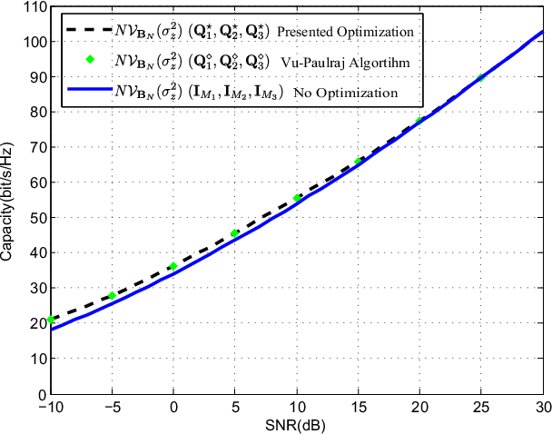
Refer to caption
Refer to caption
Refer to caption
Refer to caption
Fig. 3: Ergodic input-output mutual information versus SNRs of the WINNER II channel with (a) N1=N2=4,M1=M2=M3=4N_{1}=N_{2}=4,M_{1}=M_{2}=M_{3}=4, (b) N1=N2=32,M1=M2=M3=4N_{1}=N_{2}=32,M_{1}=M_{2}=M_{3}=4, (c) N1=N2=32,M1=M2=M3=8N_{1}=N_{2}=32,M_{1}=M_{2}=M_{3}=8 and (d) N1=N2=64,M1=M2=M3=4N_{1}=N_{2}=64,M_{1}=M_{2}=M_{3}=4. The solid lines plot the simulation results without optimization. The dashed lines denote the simulation results of the proposed algorithm, while the diamond markers denote the simulation results of the Vu-Paulraj algorithm.

Simulations are also carried out to evaluate the performance of the capacity achieving input covariance matrices (𝐐1⋆,𝐐2⋆,𝐐3⋆)(\mathbf{Q}_{1}^{\star},\mathbf{Q}_{2}^{\star},\mathbf{Q}_{3}^{\star}). Fig. 3 depicts the results of the WINNER II channel models with various system sizes. In Fig. 1 and Fig. 2, we have shown that the deterministic equivalent N​𝒱𝓑N​(σz2)N\mathcal{V}_{{\boldsymbol{\mathcal{B}}}_{N}}(\sigma_{z}^{2}) and the simulated ergodic mutual information N​𝒱𝐁N​(σz2)N\mathcal{V}_{{\mathbf{B}}_{N}}(\sigma_{z}^{2}) are nearly the same. Since the latter represents the actual performance of the input covariance matrices, we use it for producing the numerical results in Fig. 3. In all four subfigures of Fig. 3, both the ergodic mutual information N​𝒱𝐁N​(σz2)N\mathcal{V}_{\mathbf{B}_{N}}(\sigma_{z}^{2}) for (𝐐1⋆,𝐐2⋆,𝐐3⋆)(\mathbf{Q}_{1}^{\star},\mathbf{Q}_{2}^{\star},\mathbf{Q}_{3}^{\star}) and the ergodic mutual information N​𝒱𝐁N​(σz2)N\mathcal{V}_{\mathbf{B}_{N}}(\sigma_{z}^{2}) without optimization (i.e., for (𝐈M1,𝐈M2,𝐈M3)(\mathbf{I}_{M_{1}},\mathbf{I}_{M_{2}},\mathbf{I}_{M_{3}})) are shown. Let (𝐐1⋄,𝐐2⋄,𝐐3⋄)(\mathbf{Q}_{1}^{\diamond},\mathbf{Q}_{2}^{\diamond},\mathbf{Q}_{3}^{\diamond}) denote the solution of the Vu-Paulraj algorithm. The ergodic mutual information N​𝒱𝐁N​(σz2)N\mathcal{V}_{\mathbf{B}_{N}}(\sigma_{z}^{2}) for (𝐐1⋄,𝐐2⋄,𝐐3⋄)(\mathbf{Q}_{1}^{\diamond},\mathbf{Q}_{2}^{\diamond},\mathbf{Q}_{3}^{\diamond}) are also given for comparison. We note that the ergodic mutual information N​𝒱𝐁N​(σz2)N\mathcal{V}_{\mathbf{B}_{N}}(\sigma_{z}^{2}) for (𝐐1⋆,𝐐2⋆,𝐐3⋆)(\mathbf{Q}_{1}^{\star},\mathbf{Q}_{2}^{\star},\mathbf{Q}_{3}^{\star}) and that for (𝐐1⋄,𝐐2⋄,𝐐3⋄)(\mathbf{Q}_{1}^{\diamond},\mathbf{Q}_{2}^{\diamond},\mathbf{Q}_{3}^{\diamond}) are indistinguishable. We also observe that increasing the number of receive antennas decreases the optimization gain when the number of transmit antennas is fixed, whereas increasing the number of transmit antennas provides a larger gain when the number of receive antennas is fixed. The main reason behind this phenomenon is as the following: If the number of transmit antennas is fixed, then more receive antennas means lower correlations between the received channel vectors from each transmit antenna (columns of the channel matrices), and thus the performance gain provided by the optimization algorithm becomes smaller. On the other hand, if the number of receive antennas is fixed, then the received channel vectors from each transmit antenna become more correlated as the number of transmit antennas increases, and thus a larger optimization gain can be observed.

V Conclusion

In this paper, we proposed a free deterministic equivalent for the capacity analysis of a MIMO MAC with a more general channel model compared to previous works. The analysis is based on operator-valued free probability theory. We explained why the free deterministic equivalent method for the considered channel model is reasonable, and also showed how to obtain the free deterministic equivalent of the channel Gram matrix. The obtained free deterministic equivalent is an operator-valued random variable. Then, we derived the Cauchy transform of the free deterministic equivalent, the approximate Shannon transform and hence the approximate ergodic mutual information. Furthermore, we maximized the approximate ergodic mutual information to obtain the sum-rate capacity achieving input covariance matrices. Simulation results showed that the approximations are not only numerically accurate but also computationally efficient. The results of this paper can be used to design optimal precoders and evaluate the capacity or ergodic mutual information for massive MIMO uplinks with multiple antenna users.

Appendix A Prerequisites and Free Deterministic Equivalents

Free probability theory was introduced by Voiculescu as a non-commutative probability theory equipped with a notion of freeness. Voiculescu pointed out that freeness should be seen as an analogue to independence in classical probability theory [57]. Operator-valued free probability theory was also presented by Voiculescu from the very beginning in [28]. In this appendix, we briefly review definitions and results of free probability theory and operator-valued free probability theory, and introduce the free deterministic equivalents used in this paper with a rigorous mathematical justification.

A-A Free Probability and Operator-valued Free Probability

In this subsection, we briefly review definitions and results of free probability theory [36, 57] and operator-valued free probability theory [58, 57, 59, 60, 61].

Let 𝒜\mathcal{A} be a unital algebra. A non-commutative probability space (𝒜,ϕ)(\mathcal{A},\phi) consists of 𝒜\mathcal{A} and a linear functional ϕ:𝒜→ℂ\phi:\mathcal{A}\rightarrow\mathbb{C}. The elements of a non-commutative probability space are called non-commutative random variables. If 𝒜\mathcal{A} is also a C∗C^{*}-algebra and ϕ⁡(a∗​a)≥0\phi(a^{*}a)\geq 0 for all a∈𝒜a\in\mathcal{A}, then (𝒜,ϕ)(\mathcal{A},\phi) is a C∗C^{*}-probability space. An element aa of 𝒜\mathcal{A} is called a selfadjoint random variable if a=a∗a=a^{*}; an element uu of 𝒜\mathcal{A} is called a unitary random variable if u​u∗=u∗​u=1uu^{*}=u^{*}u=1; an element aa of 𝒜\mathcal{A} is called a normal random variable if a​a∗=a∗​aaa^{*}=a^{*}a.

Let (𝒜,ϕ)(\mathcal{A},\phi) be a C∗C^{*}-probability space and a∈𝒜a\in\mathcal{A} be a normal random variable. If there exists a compactly supported probability measure μa\mu_{a} on ℂ\mathbb{C} such that

∫zk​(z∗)l​d​μa​(z)=ϕ⁡(ak​(a∗)l),k,l∈ℕ\int z^{k}({z}^{*})^{l}d\mu_{a}(z)=\phi(a^{k}(a^{*})^{l}),k,l\in\mathbb{N} (130)

then μa\mu_{a} is uniquely determined and called the ∗*-distribution of aa. If aa is selfadjoint, then μa\mu_{a} is simply called the distribution of aa.

Let 𝒜1,𝒜2,⋯,𝒜n\mathcal{A}_{1},\mathcal{A}_{2},\cdots,\mathcal{A}_{n} be a family of unital subalgebras of 𝒜\mathcal{A} and kk be a positive integer. The subalgebras 𝒜i\mathcal{A}_{i} are called free or freely independent, if ϕ(x1x2⋯xk)=0\phi(x_{1}x_{2}\cdots x_{k})=0 for any kk, whenever ϕ⁡(xj)=0\phi(x_{j})=0 and xj∈𝒜i⁡(j)x_{j}\in\mathcal{A}_{i(j)} for all jj, and i⁡(j)≠i⁡(j+1)i(j)\neq i(j+1) for j=1,⋯,k−1j=1,\cdots,k-1. Let y1,y2,⋯,yn∈𝒜y_{1},y_{2},\cdots,y_{n}\in\mathcal{A}. The non-commutative random variables yiy_{i} are called free, if the unital subalgebras alg⁡(1,yi){\rm alg}(1,y_{i}) are free, where alg⁡(1,yi){\rm alg}(1,y_{i}) denotes the unital algebra generated by the random variable yiy_{i}.

Let (𝒜,ϕ)(\mathcal{A},\phi) be a C∗C^{*}-probability space, s∈𝒜s\in\mathcal{A} be a selfadjoint element and rr be a positive real number. If the distribution of ss is determined by [62]

ϕ⁡(sn)=2π​r2​∫−rrtn​r2−t2​𝑑t\phi(s^{n})=\frac{2}{\pi r^{2}}\int_{-r}^{r}t^{n}\sqrt{r^{2}-t^{2}}dt (131)

then ss is a semicircular element of radius rr. An element cc with the definition c=12​(s1+i​s2)c=\frac{1}{\sqrt{2}}(s_{1}+is_{2}) is called a circular element, if s1s_{1} and s2s_{2} are two freely independent semicircular elements with the same variance.

Let ℬ⊂𝒜\mathcal{B}\subset\mathcal{A} be a unital subalgebra. A linear map F:𝒜→ℬF:\mathcal{A}\rightarrow\mathcal{B} is a conditional expectation, if F⁡[b]=bF[b]=b for all b∈ℬb\in\mathcal{B} and F⁡[b1​𝓧​b2]=b1​F​[𝓧]​b2F[b_{1}\boldsymbol{\mathcal{X}}b_{2}]=b_{1}F[\boldsymbol{\mathcal{X}}]b_{2} for all 𝓧∈𝒜\boldsymbol{\mathcal{X}}\in\mathcal{A} and b1,b2∈ℬb_{1},b_{2}\in\mathcal{B}. An operator-valued probability space (𝒜,F)(\mathcal{A},F), also called ℬ\mathcal{B}-valued probability space, consists of ℬ⊂𝒜\mathcal{B}\subset\mathcal{A} and a conditional expectation F:𝒜→ℬF:\mathcal{A}\rightarrow\mathcal{B}. The elements of a ℬ\mathcal{B}-valued probability space are called ℬ\mathcal{B}-valued random variables. If in addition 𝒜\mathcal{A} is a C∗C^{*}-algebra, ℬ\mathcal{B} is a C∗C^{*}-subalgebra and FF is completely positive, then (𝒜,F)(\mathcal{A},F) is a ℬ\mathcal{B}-valued C∗C^{*}-probability space. Let 𝓧\boldsymbol{\mathcal{X}} be a ℬ\mathcal{B}-valued random variable of (𝒜,F)(\mathcal{A},F). The ℬ\mathcal{B}-valued distribution of 𝓧\boldsymbol{\mathcal{X}} is given by all ℬ\mathcal{B}-valued moments F[𝓧b1𝓧b2⋯𝓧bn−1𝓧]F[\boldsymbol{\mathcal{X}}b_{1}\boldsymbol{\mathcal{X}}b_{2}\cdots\boldsymbol{\mathcal{X}}b_{n-1}\boldsymbol{\mathcal{X}}], where b1,b2,⋯,bn−1∈ℬb_{1},b_{2},\cdots,b_{n-1}\in\mathcal{B}.

We denote by 𝐌n​(𝒫)\mathbf{M}_{n}(\mathcal{P}) the algebra of n×nn\times n complex random matrices. The mathematical expectation operator 𝔼\mathbb{E} over 𝐌n​(𝒫)\mathbf{M}_{n}(\mathcal{P}) is a conditional expectation from 𝐌n​(𝒫)\mathbf{M}_{n}(\mathcal{P}) to ℳn\mathcal{M}_{n}. Thus, (𝐌n​(𝒫),𝔼)(\mathbf{M}_{n}(\mathcal{P}),\mathbb{E}) is an ℳn\mathcal{M}_{n}-valued C∗C^{*}-probability space. Furthermore, (𝐌n​(𝒫),𝔼𝒟n)(\mathbf{M}_{n}(\mathcal{P}),\mathbb{E}_{\mathcal{D}_{n}}) is a 𝒟n\mathcal{D}_{n}-valued probability space, and (𝐌n​(𝒫),1n​tr∘𝔼)(\mathbf{M}_{n}(\mathcal{P}),\frac{1}{n}{\rm{tr}}\circ\mathbb{E}) or (𝐌n​(𝒫),1n​tr∘𝔼𝒟n)(\mathbf{M}_{n}(\mathcal{P}),\frac{1}{n}{\rm{tr}}\circ\mathbb{E}_{\mathcal{D}_{n}}) is a C∗C^{*}-probability space. Let 𝐗∈𝐌n​(𝒫)\mathbf{X}\in\mathbf{M}_{n}(\mathcal{P}) be a random Hermitian matrix. Then, 𝐗\mathbf{X} is at the same time an ℳn\mathcal{M}_{n}-valued, a 𝒟n\mathcal{D}_{n}-valued and a scalar valued C∗C^{*}-random variable. The ℳn\mathcal{M}_{n}-valued distribution of 𝐗\mathbf{X} determines the 𝒟n\mathcal{D}_{n}-valued distribution of 𝐗\mathbf{X}, which determines also the expected eigenvalue distribution of 𝐗\mathbf{X}.

Let 𝓧1,𝓧2,⋯,𝓧k∈(𝒜,F)\boldsymbol{\mathcal{X}}_{1},\boldsymbol{\mathcal{X}}_{2},\cdots,\boldsymbol{\mathcal{X}}_{k}\in(\mathcal{A},F) denote a family of ℬ\mathcal{B}-valued random variables and nn be a positive integer. Let AiA_{i} denote the polynomials in some 𝓧j⁡(i)\boldsymbol{\mathcal{X}}_{j(i)} with coefficients from ℬ\mathcal{B}, i.e., Ai∈ℬ⁡⟨𝓧j⁡(i)⟩A_{i}\in\mathcal{B}\langle\boldsymbol{\mathcal{X}}_{j(i)}\rangle for i=1,2,⋯,ni=1,2,\cdots,n. The ℬ\mathcal{B}-valued random variables 𝓧i\boldsymbol{\mathcal{X}}_{i} are free with amalgamation over ℬ\mathcal{B}, if F(A1A2⋯An)=0F(A_{1}A_{2}\cdots A_{n})=0 for any nn, whenever F⁡(Ai)=0F(A_{i})=0 for all ii, and j⁡(i)≠j⁡(i+1)j(i)\neq j(i+1) for i=1,⋯,n−1i=1,\cdots,n-1.

Let S⁡(n)S(n) be the finite totally ordered set {1,2,⋯,n}\{1,2,\cdots,n\} and Vi​(1≤i≤r)V_{i}(1\leq i\leq r) be pairwise disjoint subsets of S⁡(n)S(n). A set π={V1,V2,⋯,Vr}\pi=\{V_{1},V_{2},\cdots,V_{r}\} is called a partition if V1∪V2∪⋯∪Vr=S⁡(n)V_{1}\cup V_{2}\cdots\cup V_{r}=S(n). The subsets V1,V2,⋯,VrV_{1},V_{2},\cdots,V_{r} are called blocks of π\pi. The set of non-crossing partitions of S⁡(n)S(n) is denoted by N​C​(n)NC(n).

The ℬ\mathcal{B}-valued multiplicative maps {fπℬ}π∈N​C​(n):𝒜n→ℬ\{f_{\pi}^{\mathcal{B}}\}_{\pi\in NC(n)}:\mathcal{A}^{n}\rightarrow\mathcal{B} are defined recursively as

fπ1⊔π2ℬ​(𝓧1,𝓧2,⋯,𝓧n)\displaystyle\!\!\!\!f_{\pi_{1}\sqcup\pi_{2}}^{\mathcal{B}}(\boldsymbol{\mathcal{X}}_{1},\boldsymbol{\mathcal{X}}_{2},\cdots,\boldsymbol{\mathcal{X}}_{n})
=fπ1ℬ​(𝓧1,𝓧2,⋯,𝓧p)​fπ2ℬ​(𝓧p+1,𝓧p+2,⋯,𝓧n)\displaystyle=f_{\pi_{1}}^{\mathcal{B}}(\boldsymbol{\mathcal{X}}_{1},\boldsymbol{\mathcal{X}}_{2},\cdots,\boldsymbol{\mathcal{X}}_{p})f_{\pi_{2}}^{\mathcal{B}}(\boldsymbol{\mathcal{X}}_{p+1},\boldsymbol{\mathcal{X}}_{p+2},\cdots,\boldsymbol{\mathcal{X}}_{n}) (132)
fins(p,π2→π1)ℬ(𝓧1,𝓧2,⋯,𝓧n)\displaystyle\!\!\!\!f_{{\rm ins}(p,\pi_{2}\rightarrow\pi_{1})}^{\mathcal{B}}(\boldsymbol{\mathcal{X}}_{1},\boldsymbol{\mathcal{X}}_{2},\cdots,\boldsymbol{\mathcal{X}}_{n})
=fπ1ℬ​(𝓧1,𝓧2,⋯,𝓧p​fπ2ℬ​(𝓧p+1,𝓧p+2,⋯,𝓧p+q)CLOSE,\displaystyle=f_{\pi_{1}}^{\mathcal{B}}(\boldsymbol{\mathcal{X}}_{1},\boldsymbol{\mathcal{X}}_{2},\cdots,\boldsymbol{\mathcal{X}}_{p}f_{\pi_{2}}^{\mathcal{B}}(\boldsymbol{\mathcal{X}}_{p+1},\boldsymbol{\mathcal{X}}_{p+2},\cdots,\boldsymbol{\mathcal{X}}_{p+q}),
OPEN𝓧p+q+1,𝓧p+q+2,⋯,𝓧n)\displaystyle~~~~~~~~~~~~~~~~~\boldsymbol{\mathcal{X}}_{p+q+1},\boldsymbol{\mathcal{X}}_{p+q+2},\cdots,\boldsymbol{\mathcal{X}}_{n}) (133)

where π1\pi_{1} and π2\pi_{2} are two non-crossing partitions, π1⊔π2\pi_{1}\sqcup\pi_{2} denotes the disjoint union with π2\pi_{2} after π1\pi_{1}, and ins(p,π2→π1){\rm ins}(p,\pi_{2}\rightarrow\pi_{1}) denotes the partition obtained from π1\pi_{1} by inserting the partition π2\pi_{2} after the pp-th element of the set on which π1\pi_{1} determines a partition. Let 𝟏n\mathbf{1}_{n} denote {{1,2,⋯,n}}\{\{1,2,\cdots,n\}\}, 𝟎n\mathbf{0}_{n} denote {{1},{2},⋯,{n}}\{\{1\},\{2\},\cdots,\{n\}\} and fnℬ​(𝓧1,𝓧2,⋯,𝓧n)f_{n}^{\mathcal{B}}(\boldsymbol{\mathcal{X}}_{1},\boldsymbol{\mathcal{X}}_{2},\cdots,\boldsymbol{\mathcal{X}}_{n}) denote f𝟏nℬ​(𝓧1,𝓧2,⋯,𝓧n)f_{\mathbf{1}_{n}}^{\mathcal{B}}(\boldsymbol{\mathcal{X}}_{1},\boldsymbol{\mathcal{X}}_{2},\cdots,\boldsymbol{\mathcal{X}}_{n}).

Let νπℬ:𝒜n→ℬ\nu_{\pi}^{\mathcal{B}}:\mathcal{A}^{n}\rightarrow\mathcal{B} be defined by νnℬ(𝓧1,𝓧2,⋯,𝓧n)=F(𝓧1𝓧2⋯𝓧n)\nu_{n}^{\mathcal{B}}(\boldsymbol{\mathcal{X}}_{1},\boldsymbol{\mathcal{X}}_{2},\cdots,\boldsymbol{\mathcal{X}}_{n})=F(\boldsymbol{\mathcal{X}}_{1}\boldsymbol{\mathcal{X}}_{2}\cdots\boldsymbol{\mathcal{X}}_{n}). The ℬ\mathcal{B}-valued cumulants κπℬ:𝒜n→ℬ\kappa_{\pi}^{\mathcal{B}}:\mathcal{A}^{n}\rightarrow\mathcal{B}, also ℬ\mathcal{B}-valued multiplicative maps, are indirectly and inductively defined by

F(𝓧1𝓧2⋯𝓧n)=∑π∈N​C​(n)κπℬ(𝓧1,𝓧2,⋯,𝓧n).F(\boldsymbol{\mathcal{X}}_{1}\boldsymbol{\mathcal{X}}_{2}\cdots\boldsymbol{\mathcal{X}}_{n})=\sum\limits_{\pi\in NC(n)}\kappa_{\pi}^{\mathcal{B}}(\boldsymbol{\mathcal{X}}_{1},\boldsymbol{\mathcal{X}}_{2},\cdots,\boldsymbol{\mathcal{X}}_{n}). (134)

Furthermore, the ℬ\mathcal{B}-valued cumulants can be obtained from the ℬ\mathcal{B}-valued moments by

κπℬ​(𝓧1,𝓧2,⋯,𝓧n)\displaystyle\!\!\!\!\kappa_{\pi}^{\mathcal{B}}(\boldsymbol{\mathcal{X}}_{1},\boldsymbol{\mathcal{X}}_{2},\cdots,\boldsymbol{\mathcal{X}}_{n})
=∑σ≤π,σ∈N​C​(n)νσℬ​(𝓧1,𝓧2,⋯,𝓧n)​μ​(σ,π)\displaystyle=\sum\limits_{\sigma\leq\pi,\sigma\in NC(n)}\nu_{\sigma}^{\mathcal{B}}(\boldsymbol{\mathcal{X}}_{1},\boldsymbol{\mathcal{X}}_{2},\cdots,\boldsymbol{\mathcal{X}}_{n})\mu(\sigma,\pi) (135)

where σ≤π\sigma\leq\pi denotes that each block of σ\sigma is completely contained in one of the blocks of π\pi, and μ⁡(σ,π)\mu(\sigma,\pi) is the Möbius function over the non-crossing partition set N​C​(n)NC(n).

Freeness over ℬ\mathcal{B} can also be defined by using the ℬ\mathcal{B}-valued cumulants. Let S1,S2S_{1},S_{2} be two subsets of 𝒜\mathcal{A} and 𝒜i{\mathcal{A}}_{i} be the algebra generated by SiS_{i} and ℬ\mathcal{B} for i=1,2i=1,2. Then 𝒜1{\mathcal{A}}_{1} and 𝒜2{\mathcal{A}}_{2} are free with amalgamation over ℬ\mathcal{B} if and only if whenever 𝓧1,⋯,𝓧n∈S1​⋃S2\boldsymbol{\mathcal{X}}_{1},\cdots,\boldsymbol{\mathcal{X}}_{n}\in S_{1}\bigcup S_{2},

κnℬ​(𝓧1,⋯,𝓧n)=0\kappa_{n}^{\mathcal{B}}(\boldsymbol{\mathcal{X}}_{1},\cdots,\boldsymbol{\mathcal{X}}_{n})=0 (136)

unless either all 𝓧1,⋯,𝓧n∈S1\boldsymbol{\mathcal{X}}_{1},\cdots,\boldsymbol{\mathcal{X}}_{n}\in S_{1} or all 𝓧1,⋯,𝓧n∈S2\boldsymbol{\mathcal{X}}_{1},\cdots,\boldsymbol{\mathcal{X}}_{n}\in S_{2}.

Let (𝒜,ϕ)(\mathcal{A},\phi) be a non-commutative probability space and dd be a positive integer. A matrix 𝐀∈𝐌d​(𝒜)\mathbf{A}\in\mathbf{M}_{d}(\mathcal{A}) is said to be R-cyclic if the following condition holds, κnℂ​([𝐀]i1​j1,⋯,[𝐀]in​jn)=0\kappa_{n}^{\mathbb{C}}([\mathbf{A}]_{i_{1}j_{1}},\cdots,[\mathbf{A}]_{i_{n}j_{n}})=0, for every n≥1n\geq 1 and every 1≤i1,j1,⋯,in,jn≤d1\leq i_{1},j_{1},\cdots,i_{n},j_{n}\leq d for which it is not true that j1=i2,⋯,jn−1=in,jn=i1j_{1}=i_{2},\cdots,j_{n-1}=i_{n},j_{n}=i_{1} [40].

Let the operator upper half plane ℍ+​(ℬ)\mathbb{H}_{+}(\mathcal{B}) be defined by ℍ+​(ℬ)={b∈ℬ:ℑ⁡(b)≻0}\mathbb{H}_{+}(\mathcal{B})=\{b\in\mathcal{B}:\Im(b)\succ 0\}. For a selfadjoint random variable 𝓧∈𝒜\boldsymbol{\mathcal{X}}\in\mathcal{A} and b∈ℍ+​(ℬ)b\in\mathbb{H}_{+}(\mathcal{B}), the ℬ\mathcal{B}-valued Cauchy transform 𝒢𝓧ℬ​(b)\mathcal{G}_{\boldsymbol{\mathcal{X}}}^{\mathcal{B}}(b) is defined by

𝒢𝓧ℬ​(b)\displaystyle\mathcal{G}_{\boldsymbol{\mathcal{X}}}^{\mathcal{B}}(b)\!\!\!\! =\displaystyle= F​{(b−𝓧)−1}\displaystyle\!\!\!\!F\{(b-\boldsymbol{\mathcal{X}})^{-1}\} (137)
=\displaystyle= ∑n≥0F⁡{b−1​(𝓧​b−1)n},‖b−1‖≤‖𝓧‖−1.\displaystyle\!\!\!\!\sum\limits_{n\geq 0}F\{b^{-1}(\boldsymbol{\mathcal{X}}b^{-1})^{n}\},\|b^{-1}\|\leq\|\boldsymbol{\mathcal{X}}\|^{-1}.

Let the operator lower half plane ℍ−​(ℬ)\mathbb{H}_{-}(\mathcal{B}) be defined by ℍ−​(ℬ)={b∈ℬ:ℑ⁡(b)≺0}\mathbb{H}_{-}(\mathcal{B})=\{b\in\mathcal{B}:\Im(b)\prec 0\}. We have that 𝒢𝓧ℬ​(b)∈ℍ−​(ℬ)\mathcal{G}_{\boldsymbol{\mathcal{X}}}^{\mathcal{B}}(b)\in\mathbb{H}_{-}(\mathcal{B}). The ℬ\mathcal{B}-valued R-transform of 𝓧\boldsymbol{\mathcal{X}} is defined by

ℛ𝓧ℬ​(b)=∑n≥0κn+1ℬ​(𝓧​b,⋯,𝓧​b,𝓧​b,𝓧)\mathcal{R}_{\boldsymbol{\mathcal{X}}}^{\mathcal{B}}(b)=\sum\limits_{n\geq 0}\kappa_{n+1}^{\mathcal{B}}(\boldsymbol{\mathcal{X}}b,\cdots,\boldsymbol{\mathcal{X}}b,\boldsymbol{\mathcal{X}}b,\boldsymbol{\mathcal{X}}) (138)

where b∈ℍ−​(ℬ)b\in\mathbb{H}_{-}(\mathcal{B}).

Let 𝓧\boldsymbol{\mathcal{X}} and 𝓨\boldsymbol{\mathcal{Y}} be two ℬ\mathcal{B}-valued random variables. The ℬ\mathcal{B}-valued freeness relation between 𝓧\boldsymbol{\mathcal{X}} and 𝓨\boldsymbol{\mathcal{Y}} is actually a rule for calculating the mixed ℬ\mathcal{B}-valued moments in 𝓧\boldsymbol{\mathcal{X}} and 𝓨\boldsymbol{\mathcal{Y}} from the ℬ\mathcal{B}-valued moments of 𝓧\boldsymbol{\mathcal{X}} and the ℬ\mathcal{B}-valued moments of 𝓨\boldsymbol{\mathcal{Y}}. Furthermore, if 𝓧\boldsymbol{\mathcal{X}} and 𝓨\boldsymbol{\mathcal{Y}} are free over ℬ\mathcal{B}, then their mixed ℬ\mathcal{B}-valued cumulants in 𝓧\boldsymbol{\mathcal{X}} and 𝓨\boldsymbol{\mathcal{Y}} vanish. This further implies

ℛ𝓧+𝓨ℬ​(b)=ℛ𝓧ℬ​(b)+ℛ𝓨ℬ​(b).\mathcal{R}_{\boldsymbol{\mathcal{X}}+\boldsymbol{\mathcal{Y}}}^{\mathcal{B}}(b)=\mathcal{R}_{\boldsymbol{\mathcal{X}}}^{\mathcal{B}}(b)+\mathcal{R}_{\boldsymbol{\mathcal{Y}}}^{\mathcal{B}}(b). (139)

The relation between the ℬ\mathcal{B}-valued Cauchy transform and R-transform is given by

ℛ𝓧ℬ​(b)=𝒢𝓧ℬ⟨−1⟩​(b)−b−1\mathcal{R}_{\boldsymbol{\mathcal{X}}}^{\mathcal{B}}(b)={\mathcal{G}^{\mathcal{B}}_{\boldsymbol{\mathcal{X}}}}^{\langle-1\rangle}(b)-b^{-1} (140)

where 𝒢𝓧ℬ⟨−1⟩:ℍ−​(ℬ)→ℍ+​(ℬ){\mathcal{G}^{\mathcal{B}}_{\boldsymbol{\mathcal{X}}}}^{\langle-1\rangle}:\mathbb{H}_{-}(\mathcal{B})\rightarrow\mathbb{H}_{+}(\mathcal{B}) is the inverse function of 𝒢𝓧ℬ\mathcal{G}_{\boldsymbol{\mathcal{X}}}^{\mathcal{B}}. According to (140), (139) becomes

𝒢𝓧+𝓨ℬ⟨−1⟩​(b)−b−1=𝒢𝓧ℬ⟨−1⟩​(b)−b−1+ℛ𝓨ℬ​(b).{\mathcal{G}_{\boldsymbol{\mathcal{X}}+\boldsymbol{\mathcal{Y}}}^{\mathcal{B}}}^{\langle-1\rangle}(b)-b^{-1}={\mathcal{G}_{\boldsymbol{\mathcal{X}}}^{\mathcal{B}}}^{\langle-1\rangle}(b)-b^{-1}+\mathcal{R}_{\boldsymbol{\mathcal{Y}}}^{\mathcal{B}}(b). (141)

By substituting 𝒢𝓧+𝓨ℬ​(b)\mathcal{G}_{\boldsymbol{\mathcal{X}}+\boldsymbol{\mathcal{Y}}}^{\mathcal{B}}(b) for each bb, (141) becomes

b=𝒢𝓧ℬ⟨−1⟩​(𝒢𝓧+𝓨ℬ​(b))+ℛ𝓨ℬ​(𝒢𝓧+𝓨ℬ​(b))b={\mathcal{G}_{\boldsymbol{\mathcal{X}}}^{\mathcal{B}}}^{\langle-1\rangle}\left(\mathcal{G}_{\boldsymbol{\mathcal{X}}+\boldsymbol{\mathcal{Y}}}^{\mathcal{B}}(b)\right)+\mathcal{R}_{\boldsymbol{\mathcal{Y}}}^{\mathcal{B}}\left(\mathcal{G}_{\boldsymbol{\mathcal{X}}+\boldsymbol{\mathcal{Y}}}^{\mathcal{B}}(b)\right) (142)

which further leads to

𝒢𝓧+𝓨ℬ​(b)=𝒢𝓧ℬ​(b−ℛ𝓨ℬ​(𝒢𝓧+𝓨ℬ​(b))).\mathcal{G}_{\boldsymbol{\mathcal{X}}+\boldsymbol{\mathcal{Y}}}^{\mathcal{B}}(b)=\mathcal{G}_{\boldsymbol{\mathcal{X}}}^{\mathcal{B}}\left(b-\mathcal{R}_{\boldsymbol{\mathcal{Y}}}^{\mathcal{B}}\left(\mathcal{G}_{\boldsymbol{\mathcal{X}}+\boldsymbol{\mathcal{Y}}}^{\mathcal{B}}(b)\right)\right). (143)

A ℬ\mathcal{B}-valued random variable 𝓧∈𝒜\boldsymbol{\mathcal{X}}\in\mathcal{A} is called a ℬ\mathcal{B}-valued semicircular variable if its ℬ\mathcal{B}-valued R-transform is given by

ℛ𝓧ℬ​(b)=κ2ℬ​(𝓧​b,𝓧).\mathcal{R}_{\boldsymbol{\mathcal{X}}}^{\mathcal{B}}(b)=\kappa_{2}^{\mathcal{B}}(\boldsymbol{\mathcal{X}}b,\boldsymbol{\mathcal{X}}). (144)

According to (134) and (138), the higher order ℬ\mathcal{B}-valued moments of 𝓧\boldsymbol{\mathcal{X}} are given in terms of the second order moments by summing over the non-crossing pair partitions.

Let 𝓧1,𝓧2,⋯,𝓧n\boldsymbol{\mathcal{X}}_{1},\boldsymbol{\mathcal{X}}_{2},\cdots,\boldsymbol{\mathcal{X}}_{n} be a family of ℬ\mathcal{B}-valued random variables, the maps

ηi​j:𝐂→F⁡{𝓧i​𝐂​𝓧j}\eta_{ij}:\mathbf{C}\rightarrow F\{\boldsymbol{\mathcal{X}}_{i}\mathbf{C}\boldsymbol{\mathcal{X}}_{j}\}

are called the covariances of the family, where 𝐂∈ℬ\mathbf{C}\in\mathcal{B}.

A-B Free Deterministic Equivalents

In this subsection, we introduce the free deterministic equivalents for the case where all the matrices are square and have the same size, and the random matrices are Hermitian and composed of independent Gaussian entries with different variances.

Let 𝐘1,𝐘2,⋯,𝐘t\mathbf{Y}_{1},\mathbf{Y}_{2},\cdots,\mathbf{Y}_{t} be a tt-tuple of n×nn\times n Hermitian random matrices. The entries [𝐘k]i​j[\mathbf{Y}_{k}]_{ij} are Gaussian random variables. For fixed kk, the entries [𝐘k]i​j[\mathbf{Y}_{k}]_{ij} on and above the diagonal are independent, and [𝐘k]i​j=[𝐘k]j​i∗[\mathbf{Y}_{k}]_{ij}=[\mathbf{Y}_{k}]_{ji}^{*}. Moreover, the entries from different matrices are also independent. Let 1n​σi​j,k2​(n)\frac{1}{n}\sigma_{ij,k}^{2}(n) denote the variance of [𝐘k]i​j[\mathbf{Y}_{k}]_{ij}. Then, we have σi​j,k​(n)=σj​i,k​(n)\sigma_{ij,k}(n)=\sigma_{ji,k}(n) and

𝔼⁡{[𝐘k]i​j​[𝐘l]r​s}=1n​σi​j,k​(n)​σr​s,l​(n)​δj​r​δi​s​δk​l\mathbb{E}\{[\mathbf{Y}_{k}]_{ij}[\mathbf{Y}_{l}]_{rs}\}=\frac{1}{n}\sigma_{ij,k}(n)\sigma_{rs,l}(n)\delta_{jr}\delta_{is}\delta_{kl} (145)

where 1≤k,l≤t1\leq k,l\leq t and 1≤i,j,r,s≤n1\leq i,j,r,s\leq n. Let 𝐀1,𝐀2,⋯,𝐀s\mathbf{A}_{1},\mathbf{A}_{2},\cdots,\mathbf{A}_{s} be a family of n×nn\times n deterministic matrices and

Pc:=P⁡(𝐀1,𝐀2,⋯,𝐀s,𝐘1,𝐘2,⋯,𝐘t)P_{c}:=P(\mathbf{A}_{1},\mathbf{A}_{2},\cdots,\mathbf{A}_{s},{\boldsymbol{\mathbf{Y}}}_{1},{\boldsymbol{\mathbf{Y}}}_{2},\cdots,{\boldsymbol{\mathbf{Y}}}_{t})

be a selfadjoint polynomial. In the following, we will give the definition of the free deterministic equivalent of PcP_{c}.

Let 𝒜\mathcal{A} be a unital algebra, (𝒜,ϕ)(\mathcal{A},\phi) be a scalar-valued probability space and 𝓨1,𝓨2,⋯,𝓨t∈𝐌n​(𝒜)\boldsymbol{\mathcal{Y}}_{1},\boldsymbol{\mathcal{Y}}_{2},\cdots,\boldsymbol{\mathcal{Y}}_{t}\in\mathbf{M}_{n}(\mathcal{A}) be a family of selfadjoint matrices with non-commutative random variables. The entries [𝓨k]i​i[\boldsymbol{\mathcal{Y}}_{k}]_{ii} are centered semicircular elements, and the entries [𝓨k]i​j,i≠j[\boldsymbol{\mathcal{Y}}_{k}]_{ij},i\neq j, are centered circular elements. The variance of the entry [𝓨k]i​j[\boldsymbol{\mathcal{Y}}_{k}]_{ij} is given by

ϕ⁡([𝓨k]i​j​[𝓨k]i​j∗)=𝔼⁡{[𝐘k]i​j​[𝐘k]i​j∗}.\phi([\boldsymbol{\mathcal{Y}}_{k}]_{ij}[\boldsymbol{\mathcal{Y}}_{k}]_{ij}^{*})=\mathbb{E}\{[\mathbf{Y}_{k}]_{ij}[\mathbf{Y}_{k}]_{ij}^{*}\}.

Moreover, the entries on and above the diagonal of 𝓨k\boldsymbol{\mathcal{Y}}_{k} are free, and the entries from different 𝓨k\boldsymbol{\mathcal{Y}}_{k} are also free. Thus, we have

ϕ⁡([𝓨k]i​j​[𝓨l]r​s)=𝔼⁡{[𝐘k]i​j​[𝐘l]r​s}\phi([\boldsymbol{\mathcal{Y}}_{k}]_{ij}[\boldsymbol{\mathcal{Y}}_{l}]_{rs})=\mathbb{E}\{[\mathbf{Y}_{k}]_{ij}[\mathbf{Y}_{l}]_{rs}\}

where k≠lk\neq l, 1≤k,l≤t1\leq k,l\leq t and 1≤i,j,r,s≤n1\leq i,j,r,s\leq n.

According to Definition 2.92.9 of [40], 𝓨1,𝓨2,⋯,𝓨t\boldsymbol{\mathcal{Y}}_{1},\boldsymbol{\mathcal{Y}}_{2},\cdots,\boldsymbol{\mathcal{Y}}_{t} form an R-cyclic family of matrices. Then, from Theorem 8.28.2 of [40] it follows that ℳn,𝓨1,𝓨2,⋯,𝓨t\mathcal{M}_{n},\boldsymbol{\mathcal{Y}}_{1},\boldsymbol{\mathcal{Y}}_{2},\cdots,\boldsymbol{\mathcal{Y}}_{t} are free over 𝒟n\mathcal{D}_{n}. According to Theorem 7.2 of [40], we have that

κt𝒟n​(𝓨k​𝐂1,⋯,𝓨k​𝐂t−1,𝓨k)\displaystyle\!\!\!\!\!\!\!\!\kappa_{t}^{\mathcal{D}_{n}}(\boldsymbol{\mathcal{Y}}_{k}\mathbf{C}_{1},\cdots,\boldsymbol{\mathcal{Y}}_{k}\mathbf{C}_{t-1},\boldsymbol{\mathcal{Y}}_{k})
=∑i1,⋯,it=1n[𝐂1]i2​i2⋯[𝐂t−1]it​it\displaystyle=\sum\limits_{i_{1},\cdots,i_{t}=1}^{n}[\mathbf{C}_{1}]_{i_{2}i_{2}}\cdots[\mathbf{C}_{t-1}]_{i_{t}i_{t}}
κtℂ​([𝓨k]i1​i2,[𝓨k]i2​i3,⋯,[𝓨k]it​i1)​𝐏i1\displaystyle~~~~~~~~~~~~\kappa_{t}^{\mathbb{C}}([\boldsymbol{\mathcal{Y}}_{k}]_{i_{1}i_{2}},[\boldsymbol{\mathcal{Y}}_{k}]_{i_{2}i_{3}},\cdots,[\boldsymbol{\mathcal{Y}}_{k}]_{i_{t}i_{1}})\mathbf{P}_{i_{1}} (146)

where 𝐂1,⋯,𝐂t−1∈𝒟n\mathbf{C}_{1},\cdots,\mathbf{C}_{t-1}\in\mathcal{D}_{n} and 𝐏i1\mathbf{P}_{i_{1}} denotes the n×nn\times n matrix containing zeros in all entries except for the i1i_{1}-th diagonal entry, which is 11. Since the entries on and above the diagonal of 𝓨l​k\boldsymbol{\mathcal{Y}}_{lk} are a family of free (semi)circular elements and [𝓨k]i​j=[𝓨k]j​i∗[\boldsymbol{\mathcal{Y}}_{k}]_{ij}=[\boldsymbol{\mathcal{Y}}_{k}]_{ji}^{*}, we have

κtℂ​([𝓨k]i1​i2,[𝓨k]i2​i3,⋯,[𝓨k]it​i1)=0\kappa_{t}^{\mathbb{C}}([\boldsymbol{\mathcal{Y}}_{k}]_{i_{1}i_{2}},[\boldsymbol{\mathcal{Y}}_{k}]_{i_{2}i_{3}},\cdots,[\boldsymbol{\mathcal{Y}}_{k}]_{i_{t}i_{1}})=0

unless t=2t=2. Then, we obtain

κt𝒟n​(𝓨k​𝐂1,⋯,𝓨k​𝐂t−1,𝓨k)=𝟎n\kappa_{t}^{\mathcal{D}_{n}}(\boldsymbol{\mathcal{Y}}_{k}\mathbf{C}_{1},\cdots,\boldsymbol{\mathcal{Y}}_{k}\mathbf{C}_{t-1},\boldsymbol{\mathcal{Y}}_{k})=\mathbf{0}_{n}

unless t=2t=2. Thus, 𝓨1,⋯,𝓨t\boldsymbol{\mathcal{Y}}_{1},\cdots,\boldsymbol{\mathcal{Y}}_{t} are 𝒟n\mathcal{D}_{n}-valued semicircular elements.

In [59], Shlyakhtenko has proved that 𝐘1,𝐘2,⋯,𝐘t\mathbf{Y}_{1},\mathbf{Y}_{2},\cdots,\mathbf{Y}_{t} are asymptotically free over L∞​[0,1]L^{\infty}[0,1], and the asymptotic L∞​[0,1]L^{\infty}[0,1]-valued joint distribution of 𝐘1,𝐘2,⋯,𝐘t\mathbf{Y}_{1},\mathbf{Y}_{2},\cdots,\mathbf{Y}_{t} and that of 𝓨1,𝓨2,⋯,𝓨t\boldsymbol{\mathcal{Y}}_{1},\boldsymbol{\mathcal{Y}}_{2},\cdots,\boldsymbol{\mathcal{Y}}_{t} are the same. However, the proof of [59] is based on operator algebra and might be hard to understand. Thus, we present Theorem 5 in the following and prove it ourselves.

Assumption 4.

The variances σi​j,k​(n)\sigma_{ij,k}(n) are uniformly bounded in nn.

Let ψk​[n]:𝒟n→𝒟n\psi_{k}[n]:\mathcal{D}_{n}\rightarrow\mathcal{D}_{n} be defined by ψk​[n]​(𝚫n)=𝔼𝒟n​{𝐘k​𝚫n​𝐘k}\psi_{k}[n](\mathbf{\Delta}_{n})=\mathbb{E}_{\mathcal{D}_{n}}\{\mathbf{Y}_{k}\mathbf{\Delta}_{n}\mathbf{Y}_{k}\}, where 𝚫n∈𝒟n\mathbf{\Delta}_{n}\in\mathcal{D}_{n}.

Assumption 5.

There exist maps ψk:L∞​[0,1]→L∞​[0,1]\psi_{k}:L^{\infty}[0,1]\rightarrow L^{\infty}[0,1] such that whenever in​(𝚫n)→d∈L∞​[0,1]i_{n}(\mathbf{\Delta}_{n})\rightarrow d\in L^{\infty}[0,1] in norm, then also limn→∞ψk​[n]​(𝚫n)=ψk​(d)\lim_{n\rightarrow\infty}\psi_{k}[n](\mathbf{\Delta}_{n})=\psi_{k}(d).

Theorem 5.

Let mm be a positive integer. Assume that Assumption 4 holds. Then we have that

limn→∞in(𝔼𝒟n{𝐘p1𝐂1⋯𝐘pm−1𝐂m−1𝐘pm}\displaystyle\!\!\!\!\!\!\!\!\lim\limits_{n\rightarrow\infty}i_{n}(\mathbb{E}_{\mathcal{D}_{n}}\{\mathbf{Y}_{p_{1}}\mathbf{C}_{1}\cdots\mathbf{Y}_{p_{m-1}}\mathbf{C}_{m-1}\mathbf{Y}_{p_{m}}\}
−E𝒟n{𝓨p1𝐂1⋯𝓨pm−1𝐂m−1𝓨pm})=0L∞​[0,1]\displaystyle-E_{\mathcal{D}_{n}}\{\boldsymbol{\mathcal{Y}}_{p_{1}}\mathbf{C}_{1}\cdots\boldsymbol{\mathcal{Y}}_{p_{m-1}}\mathbf{C}_{m-1}\boldsymbol{\mathcal{Y}}_{p_{m}}\})=0_{L^{\infty}[0,1]} (147)

where 1≤p1,⋯,pm≤t1\leq p_{1},\cdots,p_{m}\leq t and 𝐂1,⋯,𝐂m−1\mathbf{C}_{1},\cdots,\mathbf{C}_{m-1} is a family of n×nn\times n deterministic diagonal matrices with uniformly bounded entries. Furthermore, if Assumption 5 holds, then 𝐘1,𝐘2,⋯,𝐘t\mathbf{Y}_{1},\mathbf{Y}_{2},\cdots,\mathbf{Y}_{t} are asymptotically free over L∞​[0,1]L^{\infty}[0,1].

Proof:

In [36], a proof of asymptotic freeness between Gaussian random matrices is presented. Extending the proof therein, we obtain the following results.

We first prove the special case when p1=p2=⋯=pm=kp_{1}=p_{2}=\cdots=p_{m}=k, i.e.,

limn→∞in(𝔼𝒟n{𝐘k𝐂1⋯𝐘k𝐂m−1𝐘k}\displaystyle\!\!\!\!\!\!\!\!\!\!\!\!\lim\limits_{n\rightarrow\infty}i_{n}(\mathbb{E}_{\mathcal{D}_{n}}\{\mathbf{Y}_{k}\mathbf{C}_{1}\cdots\mathbf{Y}_{k}\mathbf{C}_{m-1}\mathbf{Y}_{k}\}
−E𝒟n{𝓨k𝐂1⋯𝓨k𝐂m−1𝓨k})=0L∞​[0,1].\displaystyle-E_{\mathcal{D}_{n}}\{\boldsymbol{\mathcal{Y}}_{k}\mathbf{C}_{1}\cdots\boldsymbol{\mathcal{Y}}_{k}\mathbf{C}_{m-1}\boldsymbol{\mathcal{Y}}_{k}\})=0_{L^{\infty}[0,1]}. (148)

The 𝒟n{\mathcal{D}_{n}}-valued moment 𝔼𝒟n{𝐘k𝐂1⋯𝐘k𝐂m−1𝐘k}\mathbb{E}_{\mathcal{D}_{n}}\{\mathbf{Y}_{k}\mathbf{C}_{1}\cdots\mathbf{Y}_{k}\mathbf{C}_{m-1}\mathbf{Y}_{k}\} is given by

𝔼𝒟n{𝐘k𝐂1⋯𝐘k𝐂m−1𝐘k}\displaystyle\!\!\!\!\!\!\!\!\!\mathbb{E}_{\mathcal{D}_{n}}\{\mathbf{Y}_{k}\mathbf{C}_{1}\cdots\mathbf{Y}_{k}\mathbf{C}_{m-1}\mathbf{Y}_{k}\}
=∑i1,⋯,im=1n𝔼{[𝐘k]i1​i2[𝐂1]i2​i2⋯[𝐘k]im−1​im\displaystyle=\sum\limits_{i_{1},\cdots,i_{m}=1}^{n}\mathbb{E}\{[\mathbf{Y}_{k}]_{i_{1}i_{2}}[\mathbf{C}_{1}]_{i_{2}i_{2}}\cdots[\mathbf{Y}_{k}]_{i_{m-1}i_{m}}
[𝐂m−1]im​im[𝐘k]im​i1}𝐏i1\displaystyle~~~~~~~~~~~~~~~~[\mathbf{C}_{m-1}]_{i_{m}i_{m}}[\mathbf{Y}_{k}]_{i_{m}i_{1}}\}\mathbf{P}_{i_{1}}
=∑i1,⋯,im=1n𝔼{[𝐘k]i1​i2⋯[𝐘k]im−1​im[𝐘k]im​i1}\displaystyle=\sum\limits_{i_{1},\cdots,i_{m}=1}^{n}\mathbb{E}\{[\mathbf{Y}_{k}]_{i_{1}i_{2}}\cdots[\mathbf{Y}_{k}]_{i_{m-1}i_{m}}[\mathbf{Y}_{k}]_{i_{m}i_{1}}\}
[𝐂1]i2​i2⋯[𝐂m−1]im​im𝐏i1.\displaystyle~~~~~~~~~~~~~~~~[\mathbf{C}_{1}]_{i_{2}i_{2}}\cdots[\mathbf{C}_{m-1}]_{i_{m}i_{m}}\mathbf{P}_{i_{1}}. (149)

According to the Wick formula (Theorem 22.3 of [36]), we have that

𝔼{[𝐘k]i1​i2⋯[𝐘k]im−1​im[𝐘k]im​i1}\displaystyle\!\!\!\!\!\!\!\!\mathbb{E}\{[\mathbf{Y}_{k}]_{i_{1}i_{2}}\cdots[\mathbf{Y}_{k}]_{i_{m-1}i_{m}}[\mathbf{Y}_{k}]_{i_{m}i_{1}}\}
=∑π∈𝒫2​(m)∏(r,s)∈π𝔼⁡{[𝐘k]ir​iγ⁡(r)​[𝐘k]is​iγ⁡(s)}\displaystyle=\sum\limits_{\pi\in\mathcal{P}_{2}(m)}\prod\limits_{(r,s)\in\pi}\mathbb{E}\{[\mathbf{Y}_{k}]_{i_{r}i_{\gamma(r)}}[\mathbf{Y}_{k}]_{i_{s}i_{\gamma(s)}}\} (150)

where 𝒫2​(m)\mathcal{P}_{2}(m) denotes the set of pair partitions of S⁡(m)S(m), and γ\gamma is the cyclic permutation of S⁡(m)S(m) defined by γ⁡(i)=i+1modm\gamma(i)=i+1\mod m. Then, (149) can be rewritten as

𝔼𝒟n{𝐘k𝐂1⋯𝐘k𝐂m−1𝐘k}\displaystyle\!\!\mathbb{E}_{\mathcal{D}_{n}}\{\mathbf{Y}_{k}\mathbf{C}_{1}\cdots\mathbf{Y}_{k}\mathbf{C}_{m-1}\mathbf{Y}_{k}\}
=∑i1,⋯,im=1n∑π∈𝒫2​(m)(∏(r,s)∈π𝔼⁡{[𝐘k]ir​iγ⁡(r)​[𝐘k]is​iγ⁡(s)})\displaystyle=\!\!\sum\limits_{i_{1},\cdots,i_{m}=1}^{n}\sum\limits_{\pi\in\mathcal{P}_{2}(m)}\!\!\left(\prod\limits_{(r,s)\in\pi}\!\!\mathbb{E}\{[\mathbf{Y}_{k}]_{i_{r}i_{\gamma(r)}}[\mathbf{Y}_{k}]_{i_{s}i_{\gamma(s)}}\}\right)
[𝐂1]i2​i2⋯[𝐂m−1]im​im𝐏i1\displaystyle~~~~~~~~~~~~~~~~~~~~~~~~[\mathbf{C}_{1}]_{i_{2}i_{2}}\cdots[\mathbf{C}_{m-1}]_{i_{m}i_{m}}\mathbf{P}_{i_{1}}
=∑π∈N​C2​(m)∑i1,⋯,im=1n(∏(r,s)∈π𝔼⁡{[𝐘k]ir​iγ⁡(r)​[𝐘k]is​iγ⁡(s)})\displaystyle=\!\!\sum\limits_{\pi\in NC_{2}(m)}\sum\limits_{i_{1},\cdots,i_{m}=1}^{n}\!\!\left(\prod\limits_{(r,s)\in\pi}\!\!\mathbb{E}\{[\mathbf{Y}_{k}]_{i_{r}i_{\gamma(r)}}[\mathbf{Y}_{k}]_{i_{s}i_{\gamma(s)}}\}\right)
[𝐂1]i2​i2⋯[𝐂m−1]im​im𝐏i1\displaystyle~~~~~~~~~~~~~~~~~~~~~~~~[\mathbf{C}_{1}]_{i_{2}i_{2}}\cdots[\mathbf{C}_{m-1}]_{i_{m}i_{m}}\mathbf{P}_{i_{1}}
+∑π∈𝒫2​(m)π∉N​C2​(m)∑i1,⋯,im=1n(∏(r,s)∈π𝔼{[𝐘k]ir​iγ⁡(r)[𝐘k]is​iγ⁡(s)})\displaystyle~~~~+\!\!\!\!\sum\limits_{\begin{subarray}{c}\pi\in\mathcal{P}_{2}(m)\\ \pi\notin NC_{2}(m)\end{subarray}}\!\!\sum\limits_{i_{1},\cdots,i_{m}=1}^{n}\!\!\left(\prod\limits_{(r,s)\in\pi}\!\!\mathbb{E}\{[\mathbf{Y}_{k}]_{i_{r}i_{\gamma(r)}}[\mathbf{Y}_{k}]_{i_{s}i_{\gamma(s)}}\}\right)
[𝐂1]i2​i2⋯[𝐂m−1]im​im𝐏i1\displaystyle~~~~~~~~~~~~~~~~~~~~~~~~~~~~[\mathbf{C}_{1}]_{i_{2}i_{2}}\cdots[\mathbf{C}_{m-1}]_{i_{m}i_{m}}\mathbf{P}_{i_{1}} (151)

where N​C2​(m)⊂𝒫2​(m)NC_{2}(m)\subset\mathcal{P}_{2}(m) denotes the set of non-crossing pair partitions of S⁡(m)S(m). Meanwhile, the 𝒟n{\mathcal{D}_{n}}-valued moment E𝒟n{𝓨k𝐂1⋯𝓨k𝐂m−1𝓨k}E_{\mathcal{D}_{n}}\{\boldsymbol{\mathcal{Y}}_{k}\mathbf{C}_{1}\cdots\boldsymbol{\mathcal{Y}}_{k}\mathbf{C}_{m-1}\boldsymbol{\mathcal{Y}}_{k}\} is given by

E𝒟n{𝓨k𝐂1⋯𝓨k𝐂m−1𝓨k}\displaystyle\!\!\!\!\!\!\!\!\!\!\!\!E_{\mathcal{D}_{n}}\{\boldsymbol{\mathcal{Y}}_{k}\mathbf{C}_{1}\cdots\boldsymbol{\mathcal{Y}}_{k}\mathbf{C}_{m-1}\boldsymbol{\mathcal{Y}}_{k}\}
=∑i1,⋯,im=1nϕ([𝓨k]i1​i2[𝐂1]i2​i2⋯[𝓨k]im−1​im\displaystyle=\sum\limits_{i_{1},\cdots,i_{m}=1}^{n}\phi([\boldsymbol{\mathcal{Y}}_{k}]_{i_{1}i_{2}}[\mathbf{C}_{1}]_{i_{2}i_{2}}\cdots[\boldsymbol{\mathcal{Y}}_{k}]_{i_{m-1}i_{m}}
OPEN[𝐂m−1]im​im​[𝓨k]im​i1)​𝐏i1\displaystyle~~~~~~~~~~~~~~~~[\mathbf{C}_{m-1}]_{i_{m}i_{m}}[\boldsymbol{\mathcal{Y}}_{k}]_{i_{m}i_{1}})\mathbf{P}_{i_{1}}
=∑i1,⋯,im=1nϕ([𝓨k]i1​i2⋯[𝓨k]im−1​im[𝓨k]im​i1)\displaystyle=\sum\limits_{i_{1},\cdots,i_{m}=1}^{n}\phi([\boldsymbol{\mathcal{Y}}_{k}]_{i_{1}i_{2}}\cdots[\boldsymbol{\mathcal{Y}}_{k}]_{i_{m-1}i_{m}}[\boldsymbol{\mathcal{Y}}_{k}]_{i_{m}i_{1}})
[𝐂1]i2​i2⋯[𝐂m−1]im​im𝐏i1.\displaystyle~~~~~~~~~~~~~~~~[\mathbf{C}_{1}]_{i_{2}i_{2}}\cdots[\mathbf{C}_{m-1}]_{i_{m}i_{m}}\mathbf{P}_{i_{1}}. (152)

The entries of 𝓨k\boldsymbol{\mathcal{Y}}_{k} are a family of semicircular and circular elements. From (8.8) and (8.9) in [36], we obtain

ϕ([𝓨k]i1​i2⋯[𝓨k]im−1​im[𝓨k]im​i1)\displaystyle\!\!\!\!\!\!\!\!\phi([\boldsymbol{\mathcal{Y}}_{k}]_{i_{1}i_{2}}\cdots[\boldsymbol{\mathcal{Y}}_{k}]_{i_{m-1}i_{m}}[\boldsymbol{\mathcal{Y}}_{k}]_{i_{m}i_{1}})
=∑π∈N​C2​(m)κπℂ​([𝓨k]i1​i2,⋯,[𝓨k]im−1​im,[𝓨k]im​i1)\displaystyle=\sum\limits_{\pi\in NC_{2}(m)}\kappa_{\pi}^{\mathbb{C}}([\boldsymbol{\mathcal{Y}}_{k}]_{i_{1}i_{2}},\cdots,[\boldsymbol{\mathcal{Y}}_{k}]_{i_{m-1}i_{m}},[\boldsymbol{\mathcal{Y}}_{k}]_{i_{m}i_{1}})
=∑π∈N​C2​(m)∏(r,s)∈πϕ⁡([𝓨k]ir​iγ⁡(r)​[𝓨k]is​iγ⁡(s)).\displaystyle=\sum\limits_{\pi\in NC_{2}(m)}\prod\limits_{(r,s)\in\pi}\phi([\boldsymbol{\mathcal{Y}}_{k}]_{i_{r}i_{\gamma(r)}}[\boldsymbol{\mathcal{Y}}_{k}]_{i_{s}i_{\gamma(s)}}). (153)

Then, (152) can be rewritten as

E𝒟n{𝓨k𝐂1⋯𝓨k𝐂m−1𝓨k}\displaystyle\!\!\!\!\!\!\!\!\!\!\!\!\!\!\!\!E_{\mathcal{D}_{n}}\{\boldsymbol{\mathcal{Y}}_{k}\mathbf{C}_{1}\cdots\boldsymbol{\mathcal{Y}}_{k}\mathbf{C}_{m-1}\boldsymbol{\mathcal{Y}}_{k}\} (154)
=\displaystyle= ∑π∈N​C2​(m)∑i1,⋯,im=1n(∏(r,s)∈πϕ⁡([𝓨k]ir​iγ⁡(r)​[𝓨k]is​iγ⁡(s)))\displaystyle\!\!\!\!\!\!\!\!\sum\limits_{\pi\in NC_{2}(m)}\sum\limits_{i_{1},\cdots,i_{m}=1}^{n}\left(\prod\limits_{(r,s)\in\pi}\phi([\boldsymbol{\mathcal{Y}}_{k}]_{i_{r}i_{\gamma(r)}}[\boldsymbol{\mathcal{Y}}_{k}]_{i_{s}i_{\gamma(s)}})\right)
[𝐂1]i2​i2⋯[𝐂m−1]im​im𝐏i1.\displaystyle~~~~~~~~~~~~~~~~~~~~[\mathbf{C}_{1}]_{i_{2}i_{2}}\cdots[\mathbf{C}_{m-1}]_{i_{m}i_{m}}\mathbf{P}_{i_{1}}.

If mm is odd, then 𝒫2​(m)\mathcal{P}_{2}(m) and N​C2​(m)NC_{2}(m) are empty sets. Thus, we obtain that both 𝔼𝒟n{𝐘k𝐂1⋯𝐘k𝐂m−1𝐘k}\mathbb{E}_{\mathcal{D}_{n}}\{\mathbf{Y}_{k}\mathbf{C}_{1}\cdots\mathbf{Y}_{k}\mathbf{C}_{m-1}\mathbf{Y}_{k}\} and E𝒟n{𝓨k𝐂1⋯𝓨k𝐂m−1𝓨k}E_{\mathcal{D}_{n}}\{\boldsymbol{\mathcal{Y}}_{k}\mathbf{C}_{1}\cdots\boldsymbol{\mathcal{Y}}_{k}\mathbf{C}_{m-1}\boldsymbol{\mathcal{Y}}_{k}\} are equal to zero matrices for odd mm. Thus, we assume that mm is even for the remainder of the proof.

According to ϕ⁡([𝓨k]ir​jr​[𝓨k]is​js)=𝔼⁡{[𝐘k]ir​jr​[𝐘k]is​js}\phi([\boldsymbol{\mathcal{Y}}_{k}]_{i_{r}j_{r}}[\boldsymbol{\mathcal{Y}}_{k}]_{i_{s}j_{s}})=\mathbb{E}\{[\mathbf{Y}_{k}]_{i_{r}j_{r}}[\mathbf{Y}_{k}]_{i_{s}j_{s}}\}, (151) and (154), (148) is equivalent to that

in​(∑π∈𝒫2​(m)π∉N​C2​(m)∑i1,⋯,im=1n(∏(r,s)∈π𝔼⁡{[𝐘k]ir​iγ⁡(r)​[𝐘k]is​iγ⁡(s)})CLOSE\displaystyle i_{n}(\sum\limits_{\begin{subarray}{c}\pi\in\mathcal{P}_{2}(m)\\ \pi\notin NC_{2}(m)\end{subarray}}\sum\limits_{i_{1},\cdots,i_{m}=1}^{n}(\prod\limits_{(r,s)\in\pi}\mathbb{E}\{[\mathbf{Y}_{k}]_{i_{r}i_{\gamma(r)}}[\mathbf{Y}_{k}]_{i_{s}i_{\gamma(s)}}\})
[𝐂1]i2​i2⋯[𝐂m−1]im​im𝐏i1)\displaystyle~~~~~~~~~~~~~~~~~~~~~~~~~~~~~~~~~~[\mathbf{C}_{1}]_{i_{2}i_{2}}\cdots[\mathbf{C}_{m-1}]_{i_{m}i_{m}}\mathbf{P}_{i_{1}})

vanishes as n→∞n\rightarrow\infty. It is convenient to identify a pair partition π\pi with a special permutation by declaring the blocks of π\pi to be cycles [36]. Then, (r,s)∈π(r,s)\in\pi means π⁡(r)=s\pi(r)=s and π⁡(s)=r\pi(s)=r. Applying (145), we obtain equation (155) at the top of the following page,

∑π∈𝒫2​(m)π∉N​C2​(m)∑i1,⋯,im=1n(∏(r,s)∈π𝔼{[𝐘k]ir​iγ⁡(r)[𝐘k]is​iγ⁡(s)})[𝐂1]i2​i2⋯[𝐂m−1]im​im𝐏i1\displaystyle\!\!\!\!\!\!\!\!\sum\limits_{\begin{subarray}{c}\pi\in\mathcal{P}_{2}(m)\\ \pi\notin NC_{2}(m)\end{subarray}}\!\!\sum\limits_{i_{1},\cdots,i_{m}=1}^{n}\!\!\left(\prod\limits_{(r,s)\in\pi}\mathbb{E}\{[\mathbf{Y}_{k}]_{i_{r}i_{\gamma(r)}}[\mathbf{Y}_{k}]_{i_{s}i_{\gamma(s)}}\}\right)[\mathbf{C}_{1}]_{i_{2}i_{2}}\cdots[\mathbf{C}_{m-1}]_{i_{m}i_{m}}\mathbf{P}_{i_{1}}
=n−m2∑π∈𝒫2​(m)π∉N​C2​(m)∑i1,⋯,im=1n(∏(r,s)∈πσir​iγ⁡(r),k(n)σis​iγ⁡(s),k(n)δir​iγ⁡(s)δis​iγ⁡(r))[𝐂1]i2​i2⋯[𝐂m−1]im​im𝐏i1\displaystyle=n^{-\frac{m}{2}}\!\!\!\!\sum\limits_{\begin{subarray}{c}\pi\in\mathcal{P}_{2}(m)\\ \pi\notin NC_{2}(m)\end{subarray}}\!\!\sum\limits_{i_{1},\cdots,i_{m}=1}^{n}\!\!\left(\prod\limits_{(r,s)\in\pi}\sigma_{i_{r}i_{\gamma(r)},k}(n)\sigma_{i_{s}i_{\gamma(s)},k}(n)\delta_{i_{r}i_{\gamma(s)}}\delta_{i_{s}i_{\gamma(r)}}\right)[\mathbf{C}_{1}]_{i_{2}i_{2}}\cdots[\mathbf{C}_{m-1}]_{i_{m}i_{m}}\mathbf{P}_{i_{1}}
=n−m2∑π∈𝒫2​(m)π∉N​C2​(m)∑i1,⋯,im=1n(∏r=1mσir​iγ⁡(r),k(n)δir​iγ​π​(r))[𝐂1]i2​i2⋯[𝐂m−1]im​im𝐏i1\displaystyle=n^{-\frac{m}{2}}\!\!\!\!\sum\limits_{\begin{subarray}{c}\pi\in\mathcal{P}_{2}(m)\\ \pi\notin NC_{2}(m)\end{subarray}}\!\!\sum\limits_{i_{1},\cdots,i_{m}=1}^{n}\!\!\left(\prod\limits_{r=1}^{m}\sigma_{i_{r}i_{\gamma(r)},k}(n)\delta_{i_{r}i_{\gamma\pi(r)}}\right)[\mathbf{C}_{1}]_{i_{2}i_{2}}\cdots[\mathbf{C}_{m-1}]_{i_{m}i_{m}}\mathbf{P}_{i_{1}}
=n−m2∑π∈𝒫2​(m)π∉N​C2​(m)∑i1,⋯,im=1n(∏r=1mδir​iγ​π​(r))(∏r=1mσir​iγ⁡(r),k(n))[𝐂1]i2​i2⋯[𝐂m−1]im​im𝐏i1\displaystyle=n^{-\frac{m}{2}}\!\!\!\!\sum\limits_{\begin{subarray}{c}\pi\in\mathcal{P}_{2}(m)\\ \pi\notin NC_{2}(m)\end{subarray}}\!\!\sum\limits_{i_{1},\cdots,i_{m}=1}^{n}\!\!\left(\prod\limits_{r=1}^{m}\delta_{i_{r}i_{\gamma\pi(r)}}\right)\left(\prod\limits_{r=1}^{m}\sigma_{i_{r}i_{\gamma(r)},k}(n)\right)[\mathbf{C}_{1}]_{i_{2}i_{2}}\cdots[\mathbf{C}_{m-1}]_{i_{m}i_{m}}\mathbf{P}_{i_{1}} (155)


where γ​π\gamma\pi denotes the product of the two permutations γ\gamma and π\pi, and is defined as their composition as functions, i.e., γ​π​(r)\gamma\pi(r) denotes γ⁡(π⁡(r))\gamma(\pi(r)). Applying the triangle inequality, we then obtain

|n−m2∑i2,⋯,im=1n(∏r=1mδir​iγ​π​(r))(∏r=1mσir​iγ⁡(r),k(n))\displaystyle\!\!\!\!\!\!\!\!\left|n^{-\frac{m}{2}}\!\!\!\!\sum\limits_{i_{2},\cdots,i_{m}=1}^{n}\left(\prod\limits_{r=1}^{m}\delta_{i_{r}i_{\gamma\pi(r)}}\right)\left(\prod\limits_{r=1}^{m}\sigma_{i_{r}i_{\gamma(r)},k}(n)\right)\right.
[𝐂1]i2​i2⋯[𝐂m−1]im​im|\displaystyle~~~~~~~~~~~~~~~~~\left.\vphantom{\left|n^{-\frac{m}{2}}\sum\limits_{i_{2},\cdots,i_{m}=1}^{n}\left(\prod\limits_{r=1}^{m}\delta_{i_{r}i_{\gamma\pi(r)}}\right)\left(\prod\limits_{r=1}^{m}\sigma_{i_{r}i_{\gamma(r)},k}(n)\right)\right.}[\mathbf{C}_{1}]_{i_{2}i_{2}}\cdots[\mathbf{C}_{m-1}]_{i_{m}i_{m}}\right|
≤n−m2​∑i2,⋯,im=1n(∏r=1mδir​iγ​π​(r))​(∏r=1mσir​iγ⁡(r),k​(n))\displaystyle\leq n^{-\frac{m}{2}}\sum\limits_{i_{2},\cdots,i_{m}=1}^{n}\left(\prod\limits_{r=1}^{m}\delta_{i_{r}i_{\gamma\pi(r)}}\right)\left(\prod\limits_{r=1}^{m}\sigma_{i_{r}i_{\gamma(r)},k}(n)\right)
|[𝐂1]i2​i2⋯[𝐂m−1]im​im|\displaystyle~~~~~~~~~~~~~~~~\left|[\mathbf{C}_{1}]_{i_{2}i_{2}}\cdots[\mathbf{C}_{m-1}]_{i_{m}i_{m}}\right| (156)

where i1i_{1} is fixed. Since the entries of 𝐂1,⋯,𝐂m−1\mathbf{C}_{1},\cdots,\mathbf{C}_{m-1} and σi​j,k​(n)\sigma_{ij,k}(n) are uniformly bounded in nn, there must exists a positive real number c0c_{0} such that

|n−m2∑i2,⋯,im=1n(∏r=1mδir​iγ​π​(r))(∏r=1mσir​iγ⁡(r),k(n))\displaystyle\!\!\!\!\!\!\!\!\!\!\!\!\left|n^{-\frac{m}{2}}\sum\limits_{i_{2},\cdots,i_{m}=1}^{n}\left(\prod\limits_{r=1}^{m}\delta_{i_{r}i_{\gamma\pi(r)}}\right)\left(\prod\limits_{r=1}^{m}\sigma_{i_{r}i_{\gamma(r)},k}(n)\right)\right.
[𝐂1]i2​i2⋯[𝐂m−1]im​im|\displaystyle~~~~~~~~~~~~~~~~\left.[\mathbf{C}_{1}]_{i_{2}i_{2}}\cdots[\mathbf{C}_{m-1}]_{i_{m}i_{m}}\right|
≤c0​n−m2​∑i2,⋯,im=1n(∏r=1mδir​iγ​π​(r)).\displaystyle\leq c_{0}n^{-\frac{m}{2}}\sum\limits_{i_{2},\cdots,i_{m}=1}^{n}\left(\prod\limits_{r=1}^{m}\delta_{i_{r}i_{\gamma\pi(r)}}\right). (157)

In [36] (p.365), it is shown that

∑i1,i2,⋯,im=1n(∏r=1mδir​iγ​π​(r))=n#⁡(γ​π)\displaystyle\sum\limits_{i_{1},i_{2},\cdots,i_{m}=1}^{n}\left(\prod\limits_{r=1}^{m}\delta_{i_{r}i_{\gamma\pi(r)}}\right)=n^{\#(\gamma\pi)} (158)

where #⁡(γ​π)\#(\gamma\pi) is the number of cycles in the permutation γ​π\gamma\pi. The interpretation of (158) is as follows: For each cycle of γ​π\gamma\pi, one can choose one of the numbers 1,⋯,n1,\cdots,n for the constant value of iri_{r} on this orbit, and all these choices are independent from each other. Following the same interpretation, we have that

∑i2,⋯,im=1n(∏r=1mδir​iγ​π​(r))=n#⁡(γ​π)−1\displaystyle\sum\limits_{i_{2},\cdots,i_{m}=1}^{n}\left(\prod\limits_{r=1}^{m}\delta_{i_{r}i_{\gamma\pi(r)}}\right)=n^{\#(\gamma\pi)-1} (159)

when iri_{r} on the orbit of one cycle of γ​π\gamma\pi is fixed on i1i_{1}. If π∈𝒫2​(m)\pi\in\mathcal{P}_{2}(m), we have #⁡(γ​π)−1−m2=−2​g\#(\gamma\pi)-1-\frac{m}{2}=-2g as stated below Theorem 22.12 of [36], where g≥0g\geq 0 is called genus in the geometric language of genus expansion. The result comes from Proposition 4.2 of [63]. If π∈N​C2​(m)\pi\in NC_{2}(m), then g=0g=0 as stated in Exercise 22.14 of [36]. Furthermore, for π∈𝒫2​(m)\pi\in\mathcal{P}_{2}(m) and π∉N​C2​(m)\pi\notin NC_{2}(m), we have #⁡(γ​π)−1−m2≤−2\#(\gamma\pi)-1-\frac{m}{2}\leq-2. Thus, the RHS of the inequality in (157) is of order n−2n^{-2}, and the left-hand side (LHS) of the inequality in (157) vanishes as n→∞n\rightarrow\infty. Furthermore, (155) also vanishes and we have proven (148).

Then, we prove the general case that

limn→∞in(𝔼𝒟n{𝐘p1𝐂1⋯𝐘pm−1𝐂m−1𝐘pm}\displaystyle\!\!\!\!\!\!\!\!\!\!\lim\limits_{n\rightarrow\infty}i_{n}(\mathbb{E}_{\mathcal{D}_{n}}\{\mathbf{Y}_{p_{1}}\mathbf{C}_{1}\cdots\mathbf{Y}_{p_{m-1}}\mathbf{C}_{m-1}\mathbf{Y}_{p_{m}}\}
−E𝒟n{𝓨p1𝐂1⋯𝓨pm−1𝐂m−1𝓨pm})=0L∞​[0,1].\displaystyle\!\!-E_{\mathcal{D}_{n}}\{\boldsymbol{\mathcal{Y}}_{p_{1}}\mathbf{C}_{1}\cdots\boldsymbol{\mathcal{Y}}_{p_{m-1}}\mathbf{C}_{m-1}\boldsymbol{\mathcal{Y}}_{p_{m}}\})=0_{L^{\infty}[0,1]}. (160)

The 𝒟n\mathcal{D}_{n}-valued moment 𝔼𝒟n{𝐘p1𝐂1⋯𝐘pm−1𝐂m−1𝐘pm}\mathbb{E}_{\mathcal{D}_{n}}\{\mathbf{Y}_{p_{1}}\mathbf{C}_{1}\cdots\mathbf{Y}_{p_{m-1}}\mathbf{C}_{m-1}\mathbf{Y}_{p_{m}}\} is given by

𝔼𝒟n{𝐘p1𝐂1⋯𝐘pm−1𝐂m−1𝐘pm}\displaystyle\mathbb{E}_{\mathcal{D}_{n}}\{\mathbf{Y}_{p_{1}}\mathbf{C}_{1}\cdots\mathbf{Y}_{p_{m-1}}\mathbf{C}_{m-1}\mathbf{Y}_{p_{m}}\}
=∑π∈N​C2​(m)∑i1,⋯,im=1n∏(r,s)∈π𝔼⁡{[𝐘pr]ir​iγ⁡(r)​[𝐘ps]is​iγ⁡(s)}\displaystyle=\sum\limits_{\pi\in NC_{2}(m)}\sum\limits_{i_{1},\cdots,i_{m}=1}^{n}\prod\limits_{(r,s)\in\pi}\!\!\!\!\mathbb{E}\{[\mathbf{Y}_{p_{r}}]_{i_{r}i_{\gamma(r)}}[\mathbf{Y}_{p_{s}}]_{i_{s}i_{\gamma(s)}}\}
[𝐂1]i2​i2⋯[𝐂m−1]im​im𝐏i1\displaystyle~~~~~~~~~~~~~~~~~~~~~~~~~~~~[\mathbf{C}_{1}]_{i_{2}i_{2}}\cdots[\mathbf{C}_{m-1}]_{i_{m}i_{m}}\mathbf{P}_{i_{1}}
+∑π∈𝒫2​(m)π∉N​C2​(m)∑i1,⋯,im=1n∏(r,s)∈π𝔼{[𝐘pr]ir​iγ⁡(r)[𝐘ps]is​iγ⁡(s)}\displaystyle~~~~+\sum\limits_{\begin{subarray}{c}\pi\in\mathcal{P}_{2}(m)\\ \pi\notin NC_{2}(m)\end{subarray}}\!\!\sum\limits_{i_{1},\cdots,i_{m}=1}^{n}\prod\limits_{(r,s)\in\pi}\!\!\!\!\mathbb{E}\{[\mathbf{Y}_{p_{r}}]_{i_{r}i_{\gamma(r)}}[\mathbf{Y}_{p_{s}}]_{i_{s}i_{\gamma(s)}}\}
[𝐂1]i2​i2⋯[𝐂m−1]im​im𝐏i1.\displaystyle~~~~~~~~~~~~~~~~~~~~~~~~~~~~[\mathbf{C}_{1}]_{i_{2}i_{2}}\cdots[\mathbf{C}_{m-1}]_{i_{m}i_{m}}\mathbf{P}_{i_{1}}. (161)

To prove (160) is equivalent to prove that the second term on the RHS of (161) vanishes as n→∞n\rightarrow\infty. Then, according to (145), we have that

∑π∈𝒫2​(m)π∉N​C2​(m)∑i1,⋯,im=1n(∏(r,s)∈π𝔼⁡{[𝐘pr]ir​iγ⁡(r)​[𝐘ps]is​iγ⁡(s)})\displaystyle\!\!\!\!\sum\limits_{\begin{subarray}{c}\pi\in\mathcal{P}_{2}(m)\\ \pi\notin NC_{2}(m)\end{subarray}}\!\!\sum\limits_{i_{1},\cdots,i_{m}=1}^{n}\!\!\left(\prod\limits_{(r,s)\in\pi}\!\!\!\!\mathbb{E}\{[\mathbf{Y}_{p_{r}}]_{i_{r}i_{\gamma(r)}}[\mathbf{Y}_{p_{s}}]_{i_{s}i_{\gamma(s)}}\}\right)
[𝐂1]i2​i2⋯[𝐂m−1]im​im𝐏i1\displaystyle~~~~~~~~~~~~~~~~~~~~~~~~~[\mathbf{C}_{1}]_{i_{2}i_{2}}\cdots[\mathbf{C}_{m-1}]_{i_{m}i_{m}}\mathbf{P}_{i_{1}}
=n−m2​∑π∈𝒫2​(m)π∉N​C2​(m)∑i1,⋯,im=1n(∏(r,s)∈πσir​iγ⁡(r),pr​(n)​σis​iγ⁡(s),ps​(n)CLOSE\displaystyle=n^{-\frac{m}{2}}\!\!\!\!\!\!\sum\limits_{\begin{subarray}{c}\pi\in\mathcal{P}_{2}(m)\\ \pi\notin NC_{2}(m)\end{subarray}}\!\!\sum\limits_{i_{1},\cdots,i_{m}=1}^{n}\!\!\left(\prod\limits_{(r,s)\in\pi}\!\!\!\!\sigma_{i_{r}i_{\gamma(r)},p_{r}}(n)\sigma_{i_{s}i_{\gamma(s)},p_{s}}(n)\right.
δir​iγ⁡(s)δis​iγ⁡(r)δpr​ps)[𝐂1]i2​i2⋯[𝐂m−1]im​im𝐏i1.\displaystyle~~~~~~\left.\vphantom{\left(\prod\limits_{(r,s)\in\pi}\sigma_{i_{r}i_{\gamma(r)},p_{r}}(n)\sigma_{i_{s}i_{\gamma(s)},p_{s}}(n)\right.}\delta_{i_{r}i_{\gamma(s)}}\delta_{i_{s}i_{\gamma(r)}}\delta_{p_{r}p_{s}}\!\!\right)\!\![\mathbf{C}_{1}]_{i_{2}i_{2}}\cdots[\mathbf{C}_{m-1}]_{i_{m}i_{m}}\mathbf{P}_{i_{1}}. (162)

The above equation is similar to (155), the only difference is the extra factor δpr​ps\delta_{p_{r}p_{s}}, which just indicates that we have an extra condition on the partitions π\pi. A similar situation has been given in the proof of Proposition 22.2222.22 of [36]. Let 𝒫2(p)​(m)\mathcal{P}_{2}^{(p)}(m) and N​C2(p)​(m)NC_{2}^{(p)}(m) be defined by

𝒫2(p)(m)={π∈𝒫2(m):pr=pπ⁡(r)∀r=1,⋯,m}\mathcal{P}_{2}^{(p)}(m)=\{\pi\in\mathcal{P}_{2}(m):p_{r}=p_{{\pi(r)}}~\forall r=1,\cdots,m\}

and

NC2(p)(m)={π∈NC2(m):pr=pπ⁡(r)∀r=1,⋯,m}.NC_{2}^{(p)}(m)=\{\pi\in NC_{2}(m):p_{r}=p_{\pi(r)}~\forall r=1,\cdots,m\}.

Then, (162) becomes

∑π∈𝒫2​(m)π∉N​C2​(m)∑i1,⋯,im=1n(∏(r,s)∈π𝔼⁡{[𝐘pr]ir​iγ⁡(r)​[𝐘ps]is​iγ⁡(s)})\displaystyle\!\!\!\!\sum\limits_{\begin{subarray}{c}\pi\in\mathcal{P}_{2}(m)\\ \pi\notin NC_{2}(m)\end{subarray}}\sum\limits_{i_{1},\cdots,i_{m}=1}^{n}\left(\prod\limits_{(r,s)\in\pi}\mathbb{E}\{[\mathbf{Y}_{p_{r}}]_{i_{r}i_{\gamma(r)}}[\mathbf{Y}_{p_{s}}]_{i_{s}i_{\gamma(s)}}\}\right)
[𝐂1]i2​i2⋯[𝐂m−1]im​im𝐏i1\displaystyle~~~~~~~~~~~~~~~~~~~~~~~~~~~~[\mathbf{C}_{1}]_{i_{2}i_{2}}\cdots[\mathbf{C}_{m-1}]_{i_{m}i_{m}}\mathbf{P}_{i_{1}}
=n−m2​∑π∈𝒫2(p)​(m)π∉N​C2(p)​(m)∑i1,⋯,im=1n(∏r=1mσir​iγ⁡(r),pr​(n)​δir​iγ​π​(r))\displaystyle=n^{-\frac{m}{2}}\sum\limits_{\begin{subarray}{c}\pi\in\mathcal{P}_{2}^{(p)}(m)\\ \pi\notin NC_{2}^{(p)}(m)\end{subarray}}\sum\limits_{i_{1},\cdots,i_{m}=1}^{n}\left(\prod\limits_{r=1}^{m}\sigma_{i_{r}i_{\gamma(r)},p_{r}}(n)\delta_{i_{r}i_{\gamma\pi(r)}}\right)
[𝐂1]i2​i2⋯[𝐂m−1]im​im𝐏i1.\displaystyle~~~~~~~~~~~~~~~~~~~~~~~~~~~~[\mathbf{C}_{1}]_{i_{2}i_{2}}\cdots[\mathbf{C}_{m-1}]_{i_{m}i_{m}}\mathbf{P}_{i_{1}}. (163)

For all partitions π∈𝒫2(p)​(m)\N​C2(p)​(m)\pi\in\mathcal{P}_{2}^{(p)}(m)\backslash NC_{2}^{(p)}(m), we have that #⁡(γ​π)−1−m2≤−2\#(\gamma\pi)-1-\frac{m}{2}\leq-2. Comparing (155) with (163), we obtain that (163) vanishes as n→∞n\rightarrow\infty and furthermore (160) holds.

Since 𝓨1,𝓨2,⋯,𝓨t\boldsymbol{\mathcal{Y}}_{1},\boldsymbol{\mathcal{Y}}_{2},\cdots,\boldsymbol{\mathcal{Y}}_{t} are 𝒟n\mathcal{D}_{n}-valued semicircular elements and also free over 𝒟n\mathcal{D}_{n}, their asymptotic L∞​[0,1]L^{\infty}[0,1]-valued joint distribution is only determined by ψk,1≤k≤t\psi_{k},1\leq k\leq t. Thus, the asymptotic L∞​[0,1]L^{\infty}[0,1]-valued joint distribution of 𝓨1,𝓨2,⋯,𝓨t\boldsymbol{\mathcal{Y}}_{1},\boldsymbol{\mathcal{Y}}_{2},\cdots,\boldsymbol{\mathcal{Y}}_{t} exists. Furthermore, the asymptotic L∞​[0,1]L^{\infty}[0,1]-valued joint moments

limn→∞in(𝔼𝒟n{𝐘p1𝐂1⋯𝐘pm−1𝐂m−1𝐘pm})\lim\limits_{n\rightarrow\infty}i_{n}(\mathbb{E}_{\mathcal{D}_{n}}\{\mathbf{Y}_{p_{1}}\mathbf{C}_{1}\cdots\mathbf{Y}_{p_{m-1}}\mathbf{C}_{m-1}\mathbf{Y}_{p_{m}}\})

include all the information about the asymptotic L∞​[0,1]L^{\infty}[0,1]-valued joint distribution of 𝐘1,𝐘2,⋯,𝐘t\mathbf{Y}_{1},\mathbf{Y}_{2},\cdots,\mathbf{Y}_{t}. Thus, we obtain from (160) that the asymptotic L∞​[0,1]L^{\infty}[0,1]-valued joint distributions of 𝐘1,𝐘2,⋯,𝐘t\mathbf{Y}_{1},\mathbf{Y}_{2},\cdots,\mathbf{Y}_{t} and 𝓨1,𝓨2,⋯,𝓨t\boldsymbol{\mathcal{Y}}_{1},\boldsymbol{\mathcal{Y}}_{2},\cdots,\boldsymbol{\mathcal{Y}}_{t} are the same. Finally, we have that 𝐘1,𝐘2,⋯,𝐘t\mathbf{Y}_{1},\mathbf{Y}_{2},\cdots,\mathbf{Y}_{t} are asymptotically free over L∞​[0,1]L^{\infty}[0,1]. ∎

The asymptotic L∞​[0,1]L^{\infty}[0,1]-valued distribution of the polynomial P⁡(𝓨1,𝓨2,⋯,𝓨t)P({\boldsymbol{\mathcal{Y}}}_{1},{\boldsymbol{\mathcal{Y}}}_{2},\cdots,{\boldsymbol{\mathcal{Y}}}_{t}) is the same as the expected asymptotic L∞​[0,1]L^{\infty}[0,1]-valued distribution of P⁡(𝐘1,𝐘2,⋯,𝐘t)P(\mathbf{Y}_{1},\mathbf{Y}_{2},\cdots,\mathbf{Y}_{t}) in the sense that

limn→∞in​(𝔼𝒟n​{(P⁡(𝐘1,𝐘2,⋯,𝐘t))k}CLOSE\displaystyle\!\!\!\!\lim_{n\rightarrow\infty}i_{n}(\mathbb{E}_{\mathcal{D}_{n}}\{(P(\mathbf{Y}_{1},\mathbf{Y}_{2},\cdots,\mathbf{Y}_{t}))^{k}\}
OPEN−E𝒟n​{(P⁡(𝓨1,𝓨2,⋯,𝓨t))k})=0L∞​[0,1].\displaystyle~~~~-E_{\mathcal{D}_{n}}\{(P({\boldsymbol{\mathcal{Y}}}_{1},{\boldsymbol{\mathcal{Y}}}_{2},\cdots,{\boldsymbol{\mathcal{Y}}}_{t}))^{k}\})=0_{L^{\infty}[0,1]}. (164)

When the n×nn\times n deterministic matrices 𝐀1,𝐀2,⋯,𝐀s\mathbf{A}_{1},\mathbf{A}_{2},\cdots,\mathbf{A}_{s} are also considered, we will present Theorem 6 in the following subsection to show the asymptotic L∞​[0,1]L^{\infty}[0,1]-valued freeness of

{𝐀1,𝐀2,⋯,𝐀s},𝐘1,𝐘2,⋯,𝐘t.\{\mathbf{A}_{1},\mathbf{A}_{2},\cdots,\mathbf{A}_{s}\},\mathbf{Y}_{1},\mathbf{Y}_{2},\cdots,\mathbf{Y}_{t}.

Furthermore, Theorem 6 implies that the asymptotic L∞​[0,1]L^{\infty}[0,1]-valued distribution of

Pf:=P⁡(𝐀1,𝐀2,⋯,𝐀s,𝓨1,𝓨2,⋯,𝓨t)\displaystyle P_{f}:=P(\mathbf{A}_{1},\mathbf{A}_{2},\cdots,\mathbf{A}_{s},{\boldsymbol{\mathcal{Y}}}_{1},{\boldsymbol{\mathcal{Y}}}_{2},\cdots,{\boldsymbol{\mathcal{Y}}}_{t})

and the expected asymptotic L∞​[0,1]L^{\infty}[0,1]-valued distribution of PcP_{c} are the same. The polynomial PfP_{f} is called the free deterministic equivalent of PcP_{c}.

For finite dimensional random matrices, the difference between the 𝒟n\mathcal{D}_{n}-valued distribution of PfP_{f} and PcP_{c} is given by the deviation from 𝒟n\mathcal{D}_{n}-valued freeness of

{𝐀1,𝐀2,⋯,𝐀s},𝐘1,𝐘2,⋯,𝐘t\{\mathbf{A}_{1},\mathbf{A}_{2},\cdots,\mathbf{A}_{s}\},\mathbf{Y}_{1},\mathbf{Y}_{2},\cdots,\mathbf{Y}_{t}

and the deviation of the expected 𝒟n\mathcal{D}_{n}-valued distribution of 𝐘1,𝐘2,⋯,𝐘t\mathbf{Y}_{1},\mathbf{Y}_{2},\cdots,\mathbf{Y}_{t} from being the same as the 𝒟n\mathcal{D}_{n}-valued distribution of 𝓨1,𝓨2,⋯,𝓨t{\boldsymbol{\mathcal{Y}}}_{1},{\boldsymbol{\mathcal{Y}}}_{2},\cdots,{\boldsymbol{\mathcal{Y}}}_{t}. For large dimensional matrices, these deviations become smaller and the 𝒟n\mathcal{D}_{n}-valued distribution of PfP_{f} provides a better approximation for the expected 𝒟n\mathcal{D}_{n}-valued distribution of PcP_{c}.

A-C New Asymptotic L∞​[0,1]L^{\infty}[0,1]-valued Freeness Results

Reference [36] presents a proof of asymptotic free independence between Gaussian random matrices and deterministic matrices. We extend the proof therein and obtain the following theorem.

Assumption 6.

The spectral norms of the deterministic matrices 𝐀1,𝐀2,⋯,𝐀s\mathbf{A}_{1},\mathbf{A}_{2},\cdots,\mathbf{A}_{s} are uniformly bounded.

Theorem 6.

Let ℰn\mathcal{E}_{n} denote the algebra of n×nn\times n diagonal matrices with uniformly bounded entries and ℱn\mathcal{F}_{n} denote the algebra generated by 𝐀1,𝐀2,⋯,𝐀s\mathbf{A}_{1},\mathbf{A}_{2},\cdots,\mathbf{A}_{s} and ℰn\mathcal{E}_{n}. Let mm be a positive integer and 𝐂0,𝐂1,⋯,𝐂m∈ℱn\mathbf{C}_{0},\mathbf{C}_{1},\cdots,\mathbf{C}_{m}\in\mathcal{F}_{n} be a family of n×nn\times n deterministic matrices. Assume that Assumptions 4 and 6 hold. Then,

limn→∞in(𝔼𝒟n{𝐂0𝐘p1𝐂1𝐘p2𝐂2⋯𝐘pm𝐂m}\displaystyle\!\!\!\!\!\!\!\!\!\!\lim\limits_{n\rightarrow\infty}i_{n}(\mathbb{E}_{\mathcal{D}_{n}}\{\mathbf{C}_{0}\mathbf{Y}_{p_{1}}\mathbf{C}_{1}\mathbf{Y}_{p_{2}}\mathbf{C}_{2}\cdots\mathbf{Y}_{p_{m}}\mathbf{C}_{m}\}
−E𝒟n{𝐂0𝓨p1𝐂1𝓨p2𝐂2⋯𝓨pm𝐂m})=0L∞​[0,1]\displaystyle-E_{\mathcal{D}_{n}}\{\mathbf{C}_{0}\boldsymbol{\mathcal{Y}}_{p_{1}}\mathbf{C}_{1}\boldsymbol{\mathcal{Y}}_{p_{2}}\mathbf{C}_{2}\cdots\boldsymbol{\mathcal{Y}}_{p_{m}}\mathbf{C}_{m}\})=0_{L^{\infty}[0,1]} (165)

where 1≤p1,⋯,pm≤t1\leq p_{1},\cdots,p_{m}\leq t. Furthermore, if Assumption 5 also holds, then 𝐘1,𝐘2,⋯,𝐘t\mathbf{Y}_{1},\mathbf{Y}_{2},\cdots,\mathbf{Y}_{t}, ℱn\mathcal{F}_{n} are asymptotically free over L∞​[0,1]L^{\infty}[0,1].

Proof:

We first prove the special case when p1=p2=⋯=pm=kp_{1}=p_{2}=\cdots=p_{m}=k, i.e.,

limn→∞in(𝔼𝒟n{𝐂0𝐘k𝐂1𝐘k𝐂2⋯𝐘k𝐂m}\displaystyle\!\!\!\!\!\!\!\!\lim\limits_{n\rightarrow\infty}i_{n}(\mathbb{E}_{\mathcal{D}_{n}}\!\{\mathbf{C}_{0}\mathbf{Y}_{k}\mathbf{C}_{1}\mathbf{Y}_{k}\mathbf{C}_{2}\cdots\mathbf{Y}_{k}\mathbf{C}_{m}\}
−E𝒟n{𝐂0𝓨k𝐂1𝓨k𝐂2⋯𝓨k𝐂m})=0L∞​[0,1].\displaystyle~-E_{\mathcal{D}_{n}}\{\mathbf{C}_{0}\boldsymbol{\mathcal{Y}}_{k}\mathbf{C}_{1}\boldsymbol{\mathcal{Y}}_{k}\mathbf{C}_{2}\cdots\boldsymbol{\mathcal{Y}}_{k}\mathbf{C}_{m}\})=0_{L^{\infty}[0,1]}. (166)

Using steps similar to those used to derive (151) and (154) in the proof of Theorem 5, we obtain

𝔼𝒟n{𝐂0𝐘k𝐂1𝐘k𝐂2⋯𝐘k𝐂m}\displaystyle\!\!\!\mathbb{E}_{\mathcal{D}_{n}}\{\mathbf{C}_{0}\mathbf{Y}_{k}\mathbf{C}_{1}\mathbf{Y}_{k}\mathbf{C}_{2}\cdots\mathbf{Y}_{k}\mathbf{C}_{m}\}
=∑π∈N​C2​(m)∑i1,⋯,imj0,j1,⋯,jm=1n(∏(r,s)∈π𝔼⁡{[𝐘k]ir​jr​[𝐘k]is​js})\displaystyle=\sum\limits_{\pi\in NC_{2}(m)}\sum\limits_{\begin{subarray}{c}i_{1},\cdots,i_{m}\\ j_{0},j_{1},\cdots,j_{m}=1\end{subarray}}^{n}\left(\prod\limits_{(r,s)\in\pi}\mathbb{E}\{[\mathbf{Y}_{k}]_{i_{r}j_{r}}[\mathbf{Y}_{k}]_{i_{s}j_{s}}\}\right)
[𝐂0]j0​i1⋯[𝐂m−1]jm−1​im[𝐂m]jm​j0𝐏j0\displaystyle~~~~~~~~~~~~~~~~~[\mathbf{C}_{0}]_{j_{0}i_{1}}\cdots[\mathbf{C}_{m-1}]_{j_{m-1}i_{m}}[\mathbf{C}_{m}]_{j_{m}j_{0}}\mathbf{P}_{j_{0}}
+∑π∈𝒫2​(m)π∉N​C2​(m)∑i1,⋯,imj0,j1,⋯,jm=1n(∏(r,s)∈π𝔼{[𝐘k]ir​jr[𝐘k]is​js})\displaystyle~+\sum\limits_{\begin{subarray}{c}\pi\in\mathcal{P}_{2}(m)\\ \pi\notin NC_{2}(m)\end{subarray}}\sum\limits_{\begin{subarray}{c}i_{1},\cdots,i_{m}\\ j_{0},j_{1},\cdots,j_{m}=1\end{subarray}}^{n}\left(\prod\limits_{(r,s)\in\pi}\mathbb{E}\{[\mathbf{Y}_{k}]_{i_{r}j_{r}}[\mathbf{Y}_{k}]_{i_{s}j_{s}}\}\right)
[𝐂0]j0​i1⋯[𝐂m−1]jm−1​im[𝐂m]jm​j0𝐏j0\displaystyle~~~~~~~~~~~~~~~~~[\mathbf{C}_{0}]_{j_{0}i_{1}}\cdots[\mathbf{C}_{m-1}]_{j_{m-1}i_{m}}[\mathbf{C}_{m}]_{j_{m}j_{0}}\mathbf{P}_{j_{0}} (167)

and

E𝒟n{𝐂0𝓨k𝐂1𝓨k𝐂2⋯𝓨k𝐂m}\displaystyle\!\!\!\!E_{\mathcal{D}_{n}}\{\mathbf{C}_{0}\boldsymbol{\mathcal{Y}}_{k}\mathbf{C}_{1}\boldsymbol{\mathcal{Y}}_{k}\mathbf{C}_{2}\cdots\boldsymbol{\mathcal{Y}}_{k}\mathbf{C}_{m}\}
=∑π∈N​C2​(m)∑i1,⋯,imj0,j1,⋯,jm=1n(∏(r,s)∈πϕ⁡([𝓨k]ir​jr​[𝓨k]is​js))\displaystyle=\sum\limits_{\pi\in NC_{2}(m)}\sum\limits_{\begin{subarray}{c}i_{1},\cdots,i_{m}\\ j_{0},j_{1},\cdots,j_{m}=1\end{subarray}}^{n}\left(\prod\limits_{(r,s)\in\pi}\phi([\boldsymbol{\mathcal{Y}}_{k}]_{i_{r}j_{r}}[\boldsymbol{\mathcal{Y}}_{k}]_{i_{s}j_{s}})\right)
[𝐂0]j0​i1⋯[𝐂m−1]jm−1​im[𝐂m]jm​j0𝐏j0\displaystyle~~~~~~~~~~~~~~[\mathbf{C}_{0}]_{j_{0}i_{1}}\cdots[\mathbf{C}_{m-1}]_{j_{m-1}i_{m}}[\mathbf{C}_{m}]_{j_{m}j_{0}}\mathbf{P}_{j_{0}} (168)

respectively. Furthermore, both

𝔼𝒟n{𝐂0𝐘k𝐂1𝐘k𝐂2⋯𝐘k𝐂m}\mathbb{E}_{\mathcal{D}_{n}}\{\mathbf{C}_{0}\mathbf{Y}_{k}\mathbf{C}_{1}\mathbf{Y}_{k}\mathbf{C}_{2}\cdots\mathbf{Y}_{k}\mathbf{C}_{m}\}

and

E𝒟n{𝐂0𝓨k𝐂1𝓨k𝐂2⋯𝓨k𝐂m}E_{\mathcal{D}_{n}}\{\mathbf{C}_{0}\boldsymbol{\mathcal{Y}}_{k}\mathbf{C}_{1}\boldsymbol{\mathcal{Y}}_{k}\mathbf{C}_{2}\cdots\boldsymbol{\mathcal{Y}}_{k}\mathbf{C}_{m}\}

are equal to zero matrices for odd mm. Thus, we also assume that mm is even for the remainder of the proof.

According to ϕ⁡([𝓨k]ir​jr​[𝓨k]is​js)=𝔼⁡{[𝐘k]ir​jr​[𝐘k]is​js}\phi([\boldsymbol{\mathcal{Y}}_{k}]_{i_{r}j_{r}}[\boldsymbol{\mathcal{Y}}_{k}]_{i_{s}j_{s}})=\mathbb{E}\{[\mathbf{Y}_{k}]_{i_{r}j_{r}}[\mathbf{Y}_{k}]_{i_{s}j_{s}}\}, (167) and (168), (166) is equivalent to that

in​(∑π∈𝒫2​(m)π∉N​C2​(m)∑i1,⋯,imj0,j1,⋯,jm=1n(∏(r,s)∈π𝔼⁡{[𝐘k]ir​jr​[𝐘k]is​js})CLOSE\displaystyle\!\!\!\!\!i_{n}(\sum\limits_{\begin{subarray}{c}\pi\in\mathcal{P}_{2}(m)\\ \pi\notin NC_{2}(m)\end{subarray}}\sum\limits_{\begin{subarray}{c}i_{1},\cdots,i_{m}\\ j_{0},j_{1},\cdots,j_{m}=1\end{subarray}}^{n}(\prod\limits_{(r,s)\in\pi}\mathbb{E}\{[\mathbf{Y}_{k}]_{i_{r}j_{r}}[\mathbf{Y}_{k}]_{i_{s}j_{s}}\})
[𝐂0]j0​i1⋯[𝐂m−1]jm−1​im[𝐂m]jm​j0𝐏j0)\displaystyle~~~~~~~~~~~~~~~~~[\mathbf{C}_{0}]_{j_{0}i_{1}}\cdots[\mathbf{C}_{m-1}]_{j_{m-1}i_{m}}[\mathbf{C}_{m}]_{j_{m}j_{0}}\mathbf{P}_{j_{0}})

vanishes as n→∞n\rightarrow\infty. From (145), we then obtain equation (169) at the top of the following page.

∑π∈𝒫2​(m)π∉N​C2​(m)∑i1,⋯,imj0,j1,⋯,jm=1n(∏(r,s)∈π𝔼{[𝐘k]ir​jr[𝐘k]is​js})[𝐂0]j0​i1⋯[𝐂m−1]jm−1​im[𝐂m]jm​j0𝐏j0\displaystyle\!\!\!\!\!\!\!\!\sum\limits_{\begin{subarray}{c}\pi\in\mathcal{P}_{2}(m)\\ \pi\notin NC_{2}(m)\end{subarray}}\sum\limits_{\begin{subarray}{c}i_{1},\cdots,i_{m}\\ j_{0},j_{1},\cdots,j_{m}=1\end{subarray}}^{n}\left(\prod\limits_{(r,s)\in\pi}\mathbb{E}\{[\mathbf{Y}_{k}]_{i_{r}j_{r}}[\mathbf{Y}_{k}]_{i_{s}j_{s}}\}\right)[\mathbf{C}_{0}]_{j_{0}i_{1}}\cdots[\mathbf{C}_{m-1}]_{j_{m-1}i_{m}}[\mathbf{C}_{m}]_{j_{m}j_{0}}\mathbf{P}_{j_{0}}
=n−m2∑π∈𝒫2​(m)π∉N​C2​(m)∑i1,⋯,imj0,j1,⋯,jm=1n(∏(r,s)∈πσir​jr,k(n)σis​js,k(n)δir​jsδis​jr)[𝐂0]j0​i1⋯[𝐂m−1]jm−1​im[𝐂m]jm​j0𝐏j0\displaystyle=n^{-\frac{m}{2}}\sum\limits_{\begin{subarray}{c}\pi\in\mathcal{P}_{2}(m)\\ \pi\notin NC_{2}(m)\end{subarray}}\sum\limits_{\begin{subarray}{c}i_{1},\cdots,i_{m}\\ j_{0},j_{1},\cdots,j_{m}=1\end{subarray}}^{n}\left(\prod\limits_{(r,s)\in\pi}\sigma_{i_{r}j_{r},k}(n)\sigma_{i_{s}j_{s},k}(n)\delta_{i_{r}j_{s}}\delta_{i_{s}j_{r}}\right)[\mathbf{C}_{0}]_{j_{0}i_{1}}\cdots[\mathbf{C}_{m-1}]_{j_{m-1}i_{m}}[\mathbf{C}_{m}]_{j_{m}j_{0}}\mathbf{P}_{j_{0}}
=n−m2∑π∈𝒫2​(m)π∉N​C2​(m)∑i1,⋯,imj0,j1,⋯,jm=1n(∏r=1mσir​jr,k(n)δir​jπ⁡(r))[𝐂0]j0​i1⋯[𝐂m−1]jm−1​im[𝐂m]jm​j0𝐏j0\displaystyle=n^{-\frac{m}{2}}\sum\limits_{\begin{subarray}{c}\pi\in\mathcal{P}_{2}(m)\\ \pi\notin NC_{2}(m)\end{subarray}}\sum\limits_{\begin{subarray}{c}i_{1},\cdots,i_{m}\\ j_{0},j_{1},\cdots,j_{m}=1\end{subarray}}^{n}\left(\prod\limits_{r=1}^{m}\sigma_{i_{r}j_{r},k}(n)\delta_{i_{r}j_{{\pi(r)}}}\right)[\mathbf{C}_{0}]_{j_{0}i_{1}}\cdots[\mathbf{C}_{m-1}]_{j_{m-1}i_{m}}[\mathbf{C}_{m}]_{j_{m}j_{0}}\mathbf{P}_{j_{0}}
=n−m2∑π∈𝒫2​(m)π∉N​C2​(m)∑j0,j1,⋯,jm=1n(∏r=1mσjπ⁡(r)​jr,k(n))[𝐂0]j0​jπ​γ​(m)[𝐂1]j1​jπ​γ​(1)⋯[𝐂m−1]jm−1​jπ​γ​(m−1)[𝐂m]jm​j0𝐏j0\displaystyle=n^{-\frac{m}{2}}\!\!\!\!\!\!\sum\limits_{\begin{subarray}{c}\pi\in\mathcal{P}_{2}(m)\\ \pi\notin NC_{2}(m)\end{subarray}}\sum\limits_{j_{0},j_{1},\cdots,j_{m}=1}^{n}\left(\prod\limits_{r=1}^{m}\sigma_{j_{\pi(r)}j_{r},k}(n)\right)[\mathbf{C}_{0}]_{j_{0}j_{\pi\gamma(m)}}[\mathbf{C}_{1}]_{j_{1}j_{\pi\gamma(1)}}\cdots[\mathbf{C}_{m-1}]_{j_{m-1}j_{\pi\gamma(m-1)}}[\mathbf{C}_{m}]_{j_{m}j_{0}}\mathbf{P}_{j_{0}} (169)


Since 𝐂0,𝐂1,⋯,𝐂m\mathbf{C}_{0},\mathbf{C}_{1},\cdots,\mathbf{C}_{m} are not diagonal matrices, (169) is different from (155) in the proof of Theorem 5. Thus, the method used to prove the LHS of (155) vanishes is no longer suitable here. In the following, we use a different method to prove the LHS of (169) vanishes as n→∞n\rightarrow\infty.

If all σir​jr,k​(n)=1\sigma_{i_{r}j_{r},k}(n)=1, then (169) becomes

∑π∈𝒫2​(m)π∉N​C2​(m)∑i1,⋯,imj0,j1,⋯,jm=1n(∏(r,s)∈π𝔼⁡{[𝐘k]ir​jr​[𝐘k]is​js})\displaystyle\!\!\!\!\sum\limits_{\begin{subarray}{c}\pi\in\mathcal{P}_{2}(m)\\ \pi\notin NC_{2}(m)\end{subarray}}\sum\limits_{\begin{subarray}{c}i_{1},\cdots,i_{m}\\ j_{0},j_{1},\cdots,j_{m}=1\end{subarray}}^{n}\left(\prod\limits_{(r,s)\in\pi}\mathbb{E}\{[\mathbf{Y}_{k}]_{i_{r}j_{r}}[\mathbf{Y}_{k}]_{i_{s}j_{s}}\}\right)
[𝐂0]j0​i1⋯[𝐂m−1]jm−1​im[𝐂m]jm​j0𝐏j0\displaystyle~~~~~~~~~~~~~~~~~~~~[\mathbf{C}_{0}]_{j_{0}i_{1}}\cdots[\mathbf{C}_{m-1}]_{j_{m-1}i_{m}}[\mathbf{C}_{m}]_{j_{m}j_{0}}\mathbf{P}_{j_{0}}
=n−m2∑π∈𝒫2​(m)π∉N​C2​(m)∑j0,j1,⋯,jm=1n[𝐂0]j0​jπ​γ​(m)[𝐂1]j1​jπ​γ​(1)⋯\displaystyle~~=n^{-\frac{m}{2}}\!\!\!\!\!\!\sum\limits_{\begin{subarray}{c}\pi\in\mathcal{P}_{2}(m)\\ \pi\notin NC_{2}(m)\end{subarray}}\sum\limits_{j_{0},j_{1},\cdots,j_{m}=1}^{n}[\mathbf{C}_{0}]_{j_{0}j_{\pi\gamma(m)}}[\mathbf{C}_{1}]_{j_{1}j_{\pi\gamma(1)}}\cdots
[𝐂m−1]jm−1​jπ​γ​(m−1)​[𝐂m]jm​j0​𝐏j0.\displaystyle~~~~~~~~~~~~~~~~~~~~[\mathbf{C}_{m-1}]_{j_{m-1}j_{\pi\gamma(m-1)}}[\mathbf{C}_{m}]_{j_{m}j_{0}}\mathbf{P}_{j_{0}}. (170)

Let ρ1,ρ2,⋯,ρu\rho_{1},\rho_{2},\cdots,\rho_{u} be cycles of π​γ\pi\gamma and trπ​γ​(𝐂1,⋯,𝐂m){\rm{tr}}_{\pi\gamma}(\mathbf{C}_{1},\cdots,\mathbf{C}_{m}) be defined by

trπ​γ​(𝐂1,⋯,𝐂m)=trρ1​(𝐂1,⋯,𝐂m)​trρ2​(𝐂1,⋯,𝐂m)\displaystyle\!\!\!\!\!\!\!\!{\rm{tr}}_{\pi\gamma}(\mathbf{C}_{1},\cdots,\mathbf{C}_{m})={\rm{tr}}_{\rho_{1}}(\mathbf{C}_{1},\cdots,\mathbf{C}_{m}){\rm{tr}}_{\rho_{2}}(\mathbf{C}_{1},\cdots,\mathbf{C}_{m})
⋯trρu(𝐂1,⋯𝐂m)\displaystyle~~~~~~~~~~~~~~~~~~~~~~~~\cdots{\rm{tr}}_{\rho_{u}}(\mathbf{C}_{1},\cdots\mathbf{C}_{m}) (171)

where

trρi(𝐂1,⋯,𝐂m)=1ntr(𝐂v1𝐂v2⋯𝐂va){\rm{tr}}_{\rho_{i}}(\mathbf{C}_{1},\cdots,\mathbf{C}_{m})=\frac{1}{n}{\rm{tr}}(\mathbf{C}_{v_{1}}\mathbf{C}_{v_{2}}\cdots\mathbf{C}_{v_{a}})

if ρi=(v1,v2,⋯,va)\rho_{i}=(v_{1},v_{2},\cdots,v_{a}). Lemma 22.31 of [36] shows that

∑j1,⋯,jm=1n[𝐂1]j1​jπ​γ​(1)⋯[𝐂m−1]jm−1​jπ​γ​(m−1)[𝐂m]jm​jπ​γ​(m)\displaystyle\!\!\!\!\!\!\!\!\sum\limits_{j_{1},\cdots,j_{m}=1}^{n}[\mathbf{C}_{1}]_{j_{1}j_{\pi\gamma(1)}}\cdots[\mathbf{C}_{m-1}]_{j_{m-1}j_{\pi\gamma(m-1)}}[\mathbf{C}_{m}]_{j_{m}j_{\pi\gamma(m)}}
=n#⁡(π​γ)​trπ​γ​(𝐂1,⋯,𝐂m).\displaystyle~~~~~~~~~~~~~~~~~~~~=n^{\#(\pi\gamma)}{\rm{tr}}_{\pi\gamma}(\mathbf{C}_{1},\cdots,\mathbf{C}_{m}). (172)

For example, let m=8m=8 and π=(1,4)​(3,6)​(2,7)​(5,8)\pi=(1,4)(3,6)(2,7)(5,8). Then, we have

π​γ​(1)=π⁡(γ⁡(1))=π⁡(2)=7\displaystyle\pi\gamma(1)=\pi(\gamma(1))=\pi(2)=7
π​γ​(2)=π⁡(γ⁡(2))=π⁡(3)=6\displaystyle\pi\gamma(2)=\pi(\gamma(2))=\pi(3)=6
⋯\displaystyle~~~~~~~~~~~~~~\cdots
π​γ​(8)=π⁡(γ⁡(8))=π⁡(1)=4.\displaystyle\pi\gamma(8)=\pi(\gamma(8))=\pi(1)=4.

Then, we obtain π​γ=(4,8)​(1,7,5,3)​(2,6)\pi\gamma=(4,8)(1,7,5,3)(2,6), #⁡(π​γ)=3\#(\pi\gamma)=3 and

∑j1,⋯,j8=1n[𝐂1]j1​j7​[𝐂2]j2​j6​[𝐂3]j3​j1​[𝐂4]j4​j8\displaystyle\!\!\!\!\!\!\!\!\sum\limits_{j_{1},\cdots,j_{8}=1}^{n}[\mathbf{C}_{1}]_{j_{1}j_{7}}[\mathbf{C}_{2}]_{j_{2}j_{6}}[\mathbf{C}_{3}]_{j_{3}j_{1}}[\mathbf{C}_{4}]_{j_{4}j_{8}}
[𝐂5]j5​j3​[𝐂6]j6​j2​[𝐂7]j7​j5​[𝐂8]j8​j4\displaystyle~~~~~~~~~~~~~~~~~~~~~~~~[\mathbf{C}_{5}]_{j_{5}j_{3}}[\mathbf{C}_{6}]_{j_{6}j_{2}}[\mathbf{C}_{7}]_{j_{7}j_{5}}[\mathbf{C}_{8}]_{j_{8}j_{4}}
=∑j1,j3,j5,j7=1n[𝐂1]j1​j7​[𝐂7]j7​j5​[𝐂5]j5​j3​[𝐂3]j3​j1\displaystyle=\sum\limits_{j_{1},j_{3},j_{5},j_{7}=1}^{n}[\mathbf{C}_{1}]_{j_{1}j_{7}}[\mathbf{C}_{7}]_{j_{7}j_{5}}[\mathbf{C}_{5}]_{j_{5}j_{3}}[\mathbf{C}_{3}]_{j_{3}j_{1}}
∑j2,j6=1n[𝐂2]j2​j6​[𝐂6]j6​j2​∑j4,j8=1n[𝐂4]j4​j8​[𝐂8]j8​j4\displaystyle~~~~~~~~\sum\limits_{j_{2},j_{6}=1}^{n}[\mathbf{C}_{2}]_{j_{2}j_{6}}[\mathbf{C}_{6}]_{j_{6}j_{2}}\sum\limits_{j_{4},j_{8}=1}^{n}[\mathbf{C}_{4}]_{j_{4}j_{8}}[\mathbf{C}_{8}]_{j_{8}j_{4}}
=n3​1n​tr​(𝐂4​𝐂8)​1n​tr​(𝐂1​𝐂7​𝐂5​𝐂3)​1n​tr​(𝐂2​𝐂6)\displaystyle=n^{3}\frac{1}{n}{\rm{tr}}(\mathbf{C}_{4}\mathbf{C}_{8})\frac{1}{n}{\rm{tr}}(\mathbf{C}_{1}\mathbf{C}_{7}\mathbf{C}_{5}\mathbf{C}_{3})\frac{1}{n}{\rm{tr}}(\mathbf{C}_{2}\mathbf{C}_{6})
=n#⁡(π​γ)​trπ​γ​(𝐂1,⋯,𝐂8).\displaystyle=n^{\#(\pi\gamma)}{\rm{tr}}_{\pi\gamma}(\mathbf{C}_{1},\cdots,\mathbf{C}_{8}). (173)

From Remarks 23.8 and Proposition 23.11 of [36], we have that #⁡(π​γ)=#⁡(γ​π)\#(\pi\gamma)=\#(\gamma\pi). Without loss of generality, let ρ1=(w1,w2,⋯,wb)\rho_{1}=(w_{1},w_{2},\cdots,w_{b}) be the cycle of π​γ\pi\gamma containing mm and wb=mw_{b}=m. We denote by α\alpha the permutation ρ2∪⋯∪ρu\rho_{2}\cup\cdots\cup\rho_{u}. Then, we obtain a result similar to (172) that

n−m2∑j1,⋯,jm=1n[𝐂0]j0​jπ​γ​(m)[𝐂1]j1​jπ​γ​(1)⋯\displaystyle\!\!\!\!\!\!\!\!n^{-\frac{m}{2}}\sum\limits_{j_{1},\cdots,j_{m}=1}^{n}[\mathbf{C}_{0}]_{j_{0}j_{\pi\gamma(m)}}[\mathbf{C}_{1}]_{j_{1}j_{\pi\gamma(1)}}\cdots
[𝐂m−1]jm−1​jπ​γ​(m−1)​[𝐂m]jm​j0\displaystyle~~~~~~~~~~~~~~~~~~~~~~~~[\mathbf{C}_{m-1}]_{j_{m-1}j_{\pi\gamma(m-1)}}[\mathbf{C}_{m}]_{j_{m}j_{0}}
=n#⁡(γ​π−m2−1)trα(𝐂1,⋯,𝐂m)[𝐂0𝐂w1⋯𝐂wb]j0​j0.\displaystyle=n^{\#(\gamma\pi-\frac{m}{2}-1)}{\rm{tr}}_{\alpha}(\mathbf{C}_{1},\cdots,\mathbf{C}_{m})[\mathbf{C}_{0}\mathbf{C}_{w_{1}}\cdots\mathbf{C}_{w_{b}}]_{j_{0}j_{0}}.
(174)

Under the assumptions on 𝐂0,𝐂1,⋯,𝐂m\mathbf{C}_{0},\mathbf{C}_{1},\cdots,\mathbf{C}_{m}, the limits of all

trα(𝐂1,⋯,𝐂m)[𝐂0𝐂w1⋯𝐂wb]j0​j0{\rm{tr}}_{\alpha}(\mathbf{C}_{1},\cdots,\mathbf{C}_{m})[\mathbf{C}_{0}\mathbf{C}_{w_{1}}\cdots\mathbf{C}_{w_{b}}]_{j_{0}j_{0}}

exist. For each crossing pair partition π\pi, we have that #⁡(γ​π)−1−m2≤−2\#(\gamma\pi)-1-\frac{m}{2}\leq-2. Thus, the RHS of (170) is of order n−2n^{-2}, and the LHS of (170) vanishes as n→∞n\rightarrow\infty.

For general σir​jr,k​(n)\sigma_{i_{r}j_{r},k}(n), the formula

n−m2​∑j1,⋯,jm=1n(∏r=1mσjπ⁡(r)​jr,k​(n))​[𝐂0]j0​jπ​γ​(m)\displaystyle\!\!\!\!\!\!\!\!\!\!\!\!\!\!\!\!n^{-\frac{m}{2}}\sum\limits_{j_{1},\cdots,j_{m}=1}^{n}\left(\prod\limits_{r=1}^{m}\sigma_{j_{\pi(r)}j_{r},k}(n)\right)[\mathbf{C}_{0}]_{j_{0}j_{\pi\gamma(m)}}
[𝐂1]j1​jπ​γ​(1)⋯[𝐂m−1]jm−1​jπ​γ​(m−1)[𝐂m]jm​j0\displaystyle[\mathbf{C}_{1}]_{j_{1}j_{\pi\gamma(1)}}\cdots[\mathbf{C}_{m-1}]_{j_{m-1}j_{\pi\gamma(m-1)}}[\mathbf{C}_{m}]_{j_{m}j_{0}} (175)

is still a product of elements similar to (174) along the cycles of π​γ\pi\gamma. For example, let π=(1,4)​(2,6)​(3,7)​(5,8)\pi=(1,4)(2,6)(3,7)(5,8), m=8m=8 and π​γ=(4,8)​(1,6,3)​(2,7,5)\pi\gamma=(4,8)(1,6,3)(2,7,5). Then, we obtain equation (176) at the top of the following page,

n−4∑j1,⋯,j8=1n(∏r=18σjπ⁡(r)​jr,k(n))[𝐂0]j0​jπ​γ​(8)[𝐂1]j1​jπ​γ​(1)⋯[𝐂m−1]j7​jπ​γ​(7)[𝐂m]j8​j0\displaystyle\!\!\!\!n^{-4}\sum\limits_{j_{1},\cdots,j_{8}=1}^{n}\left(\prod\limits_{r=1}^{8}\sigma_{j_{\pi(r)}j_{r},k}(n)\right)[\mathbf{C}_{0}]_{j_{0}j_{\pi\gamma(8)}}[\mathbf{C}_{1}]_{j_{1}j_{\pi\gamma(1)}}\cdots[\mathbf{C}_{m-1}]_{j_{7}j_{\pi\gamma(7)}}[\mathbf{C}_{m}]_{j_{8}j_{0}}
=n−4​∑j1,⋯,j8=1n([𝐂3]j3​j1​[𝚲j4]j1​j1​[𝐂1]j1​j6​[𝚲j2]j6​j6​[𝐂6]j6​j3)​([𝐂2]j2​j7​[𝚲j3]j7​j7​[𝐂7]j7​j5​[𝚲j8]j5​j5​[𝐂5]j5​j2)\displaystyle=n^{-4}\sum\limits_{j_{1},\cdots,j_{8}=1}^{n}\left([\mathbf{C}_{3}]_{j_{3}j_{1}}[\mathbf{\Lambda}_{j_{4}}]_{j_{1}j_{1}}[\mathbf{C}_{1}]_{j_{1}j_{6}}[\mathbf{\Lambda}_{j_{2}}]_{j_{6}j_{6}}[\mathbf{C}_{6}]_{j_{6}j_{3}}\right)\left([\mathbf{C}_{2}]_{j_{2}j_{7}}[\mathbf{\Lambda}_{j_{3}}]_{j_{7}j_{7}}[\mathbf{C}_{7}]_{j_{7}j_{5}}[\mathbf{\Lambda}_{j_{8}}]_{j_{5}j_{5}}[\mathbf{C}_{5}]_{j_{5}j_{2}}\right)
([𝐂0]j0​j4​[𝐂4]j4​j8​[𝐂8]j8​j0)\displaystyle~~~~~~~~~~~~~~~~~~~~~~~~~~~~~~~~~\left([\mathbf{C}_{0}]_{j_{0}j_{4}}[\mathbf{C}_{4}]_{j_{4}j_{8}}[\mathbf{C}_{8}]_{j_{8}j_{0}}\right)
=n−4​∑j0,j2,j3,j4,j8=1n([𝐂3​𝚲j4​𝐂1​𝚲j2​𝐂6]j3​j3)​([𝐂2​𝚲j3​𝐂7​𝚲j8​𝐂5]j2​j2)​([𝐂0]j0​j4​[𝐂4]j4​j8​[𝐂8]j8​j0)\displaystyle=n^{-4}\sum\limits_{j_{0},j_{2},j_{3},j_{4},j_{8}=1}^{n}\left([\mathbf{C}_{3}\mathbf{\Lambda}_{j_{4}}\mathbf{C}_{1}\mathbf{\Lambda}_{j_{2}}\mathbf{C}_{6}]_{j_{3}j_{3}}\right)\left([\mathbf{C}_{2}\mathbf{\Lambda}_{j_{3}}\mathbf{C}_{7}\mathbf{\Lambda}_{j_{8}}\mathbf{C}_{5}]_{j_{2}j_{2}}\right)\left([\mathbf{C}_{0}]_{j_{0}j_{4}}[\mathbf{C}_{4}]_{j_{4}j_{8}}[\mathbf{C}_{8}]_{j_{8}j_{0}}\right)
=n−2​∑j2,j3=1n1n2​[𝐂0​𝚵j2​j3​𝐂4​𝚺j2​j3​𝐂8]j0​j0\displaystyle=n^{-2}\sum\limits_{j_{2},j_{3}=1}^{n}\frac{1}{n^{2}}[\mathbf{C}_{0}\mathbf{\Xi}_{j_{2}j_{3}}\mathbf{C}_{4}\mathbf{\Sigma}_{j_{2}j_{3}}\mathbf{C}_{8}]_{j_{0}j_{0}} (176)


where

𝚲jr=diag⁡(σ1​jr,k2​(n),σ2​jr,k2​(n),⋯,σn​jr,k2​(n))\displaystyle\mathbf{\Lambda}_{j_{r}}={\rm{diag}}(\sigma_{1j_{r},k}^{2}(n),\sigma_{2j_{r},k}^{2}(n),\cdots,\sigma_{nj_{r},k}^{2}(n))
𝚵j2​j3=diag⁡([𝐂3​𝚲1​𝐂1​𝚲j2​𝐂6]j3​j3,[𝐂3​𝚲2​𝐂1​𝚲j2​𝐂6]j3​j3CLOSE\displaystyle\mathbf{\Xi}_{j_{2}j_{3}}={\rm{diag}}([\mathbf{C}_{3}\mathbf{\Lambda}_{1}\mathbf{C}_{1}\mathbf{\Lambda}_{j_{2}}\mathbf{C}_{6}]_{j_{3}j_{3}},[\mathbf{C}_{3}\mathbf{\Lambda}_{2}\mathbf{C}_{1}\mathbf{\Lambda}_{j_{2}}\mathbf{C}_{6}]_{j_{3}j_{3}}
OPEN⋯,[𝐂3​𝚲n​𝐂1​𝚲j2​𝐂6]j3​j3)\displaystyle~~~~~~~~~~~~~~~~~~~~~~~~~~~~~~~~\cdots,[\mathbf{C}_{3}\mathbf{\Lambda}_{n}\mathbf{C}_{1}\mathbf{\Lambda}_{j_{2}}\mathbf{C}_{6}]_{j_{3}j_{3}})
𝚺j2​j3=diag⁡([𝐂2​𝚲j3​𝐂7​𝚲1​𝐂5]j2​j2,[𝐂2​𝚲j3​𝐂7​𝚲2​𝐂5]j2​j2CLOSE\displaystyle\mathbf{\Sigma}_{j_{2}j_{3}}={\rm{diag}}([\mathbf{C}_{2}\mathbf{\Lambda}_{j_{3}}\mathbf{C}_{7}\mathbf{\Lambda}_{1}\mathbf{C}_{5}]_{j_{2}j_{2}},[\mathbf{C}_{2}\mathbf{\Lambda}_{j_{3}}\mathbf{C}_{7}\mathbf{\Lambda}_{2}\mathbf{C}_{5}]_{j_{2}j_{2}}
OPEN⋯,[𝐂2​𝚲j3​𝐂7​𝚲n​𝐂5]j2​j2).\displaystyle~~~~~~~~~~~~~~~~~~~~~~~~~~~~~~~~\cdots,[\mathbf{C}_{2}\mathbf{\Lambda}_{j_{3}}\mathbf{C}_{7}\mathbf{\Lambda}_{n}\mathbf{C}_{5}]_{j_{2}j_{2}}).

Thus, (175) is still of order n#⁡(γ​π)−1−m2n^{\#(\gamma\pi)-1-\frac{m}{2}}, and the LHS of (170) is of order n−2n^{-2}. Furthermore, we have proven that (166) holds.

Then, we continue to prove the situation with more than one random matrix that

limn→∞in(𝔼𝒟n{𝐂0𝐘p1𝐂1𝐘p2𝐂2⋯𝐘pm𝐂m}\displaystyle\lim\limits_{n\rightarrow\infty}i_{n}(\mathbb{E}_{\mathcal{D}_{n}}\{\mathbf{C}_{0}\mathbf{Y}_{p_{1}}\mathbf{C}_{1}\mathbf{Y}_{p_{2}}\mathbf{C}_{2}\cdots\mathbf{Y}_{p_{m}}\mathbf{C}_{m}\}
−𝔼𝒟n{𝐂0𝓨p1𝐂1𝓨p2𝐂2⋯𝓨pm𝐂m})=0L∞​[0,1].\displaystyle~~~~~~~~-\mathbb{E}_{\mathcal{D}_{n}}\{\mathbf{C}_{0}\boldsymbol{\mathcal{Y}}_{p_{1}}\mathbf{C}_{1}\boldsymbol{\mathcal{Y}}_{p_{2}}\mathbf{C}_{2}\cdots\boldsymbol{\mathcal{Y}}_{p_{m}}\mathbf{C}_{m}\})=0_{L^{\infty}[0,1]}.
(177)

The proof of (177) is similar to that of (160) in the proof of Theorem 5 and omitted here for brevity.

Since ℳn,𝓨1,𝓨2,⋯,𝓨t\mathcal{M}_{n},\boldsymbol{\mathcal{Y}}_{1},\boldsymbol{\mathcal{Y}}_{2},\cdots,\boldsymbol{\mathcal{Y}}_{t} are free over 𝒟n\mathcal{D}_{n} and ℱn⊂ℳn\mathcal{F}_{n}\subset\mathcal{M}_{n}, we obtain that ℱn,𝓨1,𝓨2,⋯,𝓨t\mathcal{F}_{n},\boldsymbol{\mathcal{Y}}_{1},\boldsymbol{\mathcal{Y}}_{2},\cdots,\boldsymbol{\mathcal{Y}}_{t} are free over 𝒟n\mathcal{D}_{n}. Then, since 𝓨1,𝓨2,⋯,𝓨t\boldsymbol{\mathcal{Y}}_{1},\boldsymbol{\mathcal{Y}}_{2},\cdots,\boldsymbol{\mathcal{Y}}_{t} are 𝒟n\mathcal{D}_{n}-valued semicircular elements, we have that the asymptotic L∞​[0,1]L^{\infty}[0,1]-valued joint distribution of ℱn,𝓨1,𝓨2,⋯,𝓨t\mathcal{F}_{n},\boldsymbol{\mathcal{Y}}_{1},\boldsymbol{\mathcal{Y}}_{2},\cdots,\boldsymbol{\mathcal{Y}}_{t} is only determined by ψk\psi_{k} and the asymptotic L∞​[0,1]L^{\infty}[0,1]-valued joint distribution of elements from ℱn\mathcal{F}_{n}. Furthermore, the elements of ℱn\mathcal{F}_{n} have uniformly bounded spectral norm. Thus, the asymptotic L∞​[0,1]L^{\infty}[0,1]-valued joint distribution of ℱn,𝓨1,𝓨2,⋯,𝓨t\mathcal{F}_{n},\boldsymbol{\mathcal{Y}}_{1},\boldsymbol{\mathcal{Y}}_{2},\cdots,\boldsymbol{\mathcal{Y}}_{t} exists. Then, since the asymptotic L∞​[0,1]L^{\infty}[0,1]-valued joint moments

limn→∞in(𝔼𝒟n{𝐂0𝐘p1𝐂1⋯𝐘pm−1𝐂m−1𝐘pm𝐂m})\lim\limits_{n\rightarrow\infty}i_{n}(\mathbb{E}_{\mathcal{D}_{n}}\{\mathbf{C}_{0}\mathbf{Y}_{p_{1}}\mathbf{C}_{1}\cdots\mathbf{Y}_{p_{m-1}}\mathbf{C}_{m-1}\mathbf{Y}_{p_{m}}\mathbf{C}_{m}\})

include all the information about the asymptotic L∞​[0,1]L^{\infty}[0,1]-valued joint distribution of ℱn,𝐘1,𝐘2,⋯,𝐘t\mathcal{F}_{n},\mathbf{Y}_{1},\mathbf{Y}_{2},\cdots,\mathbf{Y}_{t}, we obtain from (177) that the asymptotic L∞​[0,1]L^{\infty}[0,1]-valued joint distributions of ℱn,𝐘1,𝐘2,⋯,𝐘t\mathcal{F}_{n},\mathbf{Y}_{1},\mathbf{Y}_{2},\cdots,\mathbf{Y}_{t} and ℱn,𝓨1,𝓨2,⋯,𝓨t\mathcal{F}_{n},\boldsymbol{\mathcal{Y}}_{1},\boldsymbol{\mathcal{Y}}_{2},\cdots,\boldsymbol{\mathcal{Y}}_{t} are the same. Thus, we have that ℱn,𝐘1,𝐘2,⋯,𝐘t\mathcal{F}_{n},\mathbf{Y}_{1},\mathbf{Y}_{2},\cdots,\mathbf{Y}_{t} are asymptotically free over L∞​[0,1]L^{\infty}[0,1]. ∎

Appendix B Proof of Lemma 1

From Definition 2.92.9 of [40], we have that 𝓨11,⋯,𝓨L​K\boldsymbol{\mathcal{Y}}_{11},\cdots,\boldsymbol{\mathcal{Y}}_{LK} form an R-cyclic family of matrices. Applying Theorem 8.28.2 of [40], we then obtain ℳn,𝓨11,⋯,𝓨L​K\mathcal{M}_{n},\boldsymbol{\mathcal{Y}}_{11},\cdots,\boldsymbol{\mathcal{Y}}_{LK} are free over 𝒟n\mathcal{D}_{n}. The joint ℳn\mathcal{M}_{n}-valued cumulants of 𝓧^11,⋯,𝓧^L​K\widehat{\boldsymbol{\mathcal{X}}}_{11},\cdots,\widehat{\boldsymbol{\mathcal{X}}}_{LK} are given by

κtℳn​(𝓧^i1​j1​𝐂1,𝓧^i2​j2​𝐂2,⋯,𝓧^it​jt)\displaystyle\!\!\!\!\kappa_{t}^{\mathcal{M}_{n}}(\widehat{\boldsymbol{\mathcal{X}}}_{i_{1}j_{1}}\mathbf{C}_{1},\widehat{\boldsymbol{\mathcal{X}}}_{i_{2}j_{2}}\mathbf{C}_{2},\cdots,\widehat{\boldsymbol{\mathcal{X}}}_{i_{t}j_{t}})
=κtℳn​(𝐀i1​j1​𝓨i1​j1​𝐀i1​j1H​𝐂1,𝐀i2​j2​𝓨i2​j2​𝐀i2​j2H​𝐂2CLOSE,\displaystyle~=\kappa_{t}^{\mathcal{M}_{n}}(\mathbf{A}_{i_{1}j_{1}}\boldsymbol{\mathcal{Y}}_{i_{1}j_{1}}\mathbf{A}_{i_{1}j_{1}}^{H}\mathbf{C}_{1},\mathbf{A}_{i_{2}j_{2}}\boldsymbol{\mathcal{Y}}_{i_{2}j_{2}}\mathbf{A}_{i_{2}j_{2}}^{H}\mathbf{C}_{2},
OPEN⋯,𝐀it​jt​𝓨it​jt​𝐀it​jtH)\displaystyle~~~~~~~~~~~~~~~~~~~~~~~~~~~~~~~~~~\cdots,\mathbf{A}_{i_{t}j_{t}}\boldsymbol{\mathcal{Y}}_{i_{t}j_{t}}\mathbf{A}_{i_{t}j_{t}}^{H})
=𝐀i1​j1​κtℳn​(𝓨i1​j1​𝐀i1​j1H​𝐂1​𝐀i2​j2,𝓨i2​j2​𝐀i2​j2H​𝐂2​𝐀i3​j3CLOSE,\displaystyle~=\mathbf{A}_{i_{1}j_{1}}\kappa_{t}^{\mathcal{M}_{n}}(\boldsymbol{\mathcal{Y}}_{i_{1}j_{1}}\mathbf{A}_{i_{1}j_{1}}^{H}\mathbf{C}_{1}\mathbf{A}_{i_{2}j_{2}},\boldsymbol{\mathcal{Y}}_{i_{2}j_{2}}\mathbf{A}_{i_{2}j_{2}}^{H}\mathbf{C}_{2}\mathbf{A}_{i_{3}j_{3}},
OPEN⋯,𝓨it​jt)​𝐀it​jtH\displaystyle~~~~~~~~~~~~~~~~~~~~~~~~~~~~~~~~~~\cdots,\boldsymbol{\mathcal{Y}}_{i_{t}j_{t}})\mathbf{A}_{i_{t}j_{t}}^{H}
=𝐀i1​j1​κt𝒟n​(𝓨i1​j1​E𝒟n​{𝐀i1​j1H​𝐂1​𝐀i2​j2},𝓨i2​j2CLOSE\displaystyle~=\mathbf{A}_{i_{1}j_{1}}\kappa_{t}^{\mathcal{D}_{n}}(\boldsymbol{\mathcal{Y}}_{i_{1}j_{1}}E_{\mathcal{D}_{n}}\{\mathbf{A}_{i_{1}j_{1}}^{H}\mathbf{C}_{1}\mathbf{A}_{i_{2}j_{2}}\},\boldsymbol{\mathcal{Y}}_{i_{2}j_{2}}
OPENE𝒟n​{𝐀i2​j2H​𝐂2​𝐀i3​j3},⋯,𝓨it​jt)​𝐀it​jtH\displaystyle~~~~~~~~~~~~~~E_{\mathcal{D}_{n}}\{\mathbf{A}_{i_{2}j_{2}}^{H}\mathbf{C}_{2}\mathbf{A}_{i_{3}j_{3}}\},\cdots,\boldsymbol{\mathcal{Y}}_{i_{t}j_{t}})\mathbf{A}_{i_{t}j_{t}}^{H} (178)

where 1≤it≤L1\leq i_{t}\leq L, 1≤jt≤K1\leq j_{t}\leq K, 𝐂1,𝐂2,⋯,𝐂t∈ℳn\mathbf{C}_{1},\mathbf{C}_{2},\cdots,\mathbf{C}_{t}\in\mathcal{M}_{n}, and the last equality is obtained by applying Theorem 3.63.6 of [29], which requires that ℳn\mathcal{M}_{n} and {𝓨11,⋯,𝓨L​K}\{\boldsymbol{\mathcal{Y}}_{11},\cdots,\boldsymbol{\mathcal{Y}}_{LK}\} are free over 𝒟n\mathcal{D}_{n}. Since κt𝒟n∈𝒟n\kappa_{t}^{\mathcal{D}_{n}}\in{\mathcal{D}_{n}}, we obtain

κtℳn​(𝓧^i1​j1​𝐂𝟏,𝓧^i2​j2​𝐂𝟐,⋯,𝓧^it​jt)∈𝒟.\kappa_{t}^{\mathcal{M}_{n}}(\widehat{\boldsymbol{\mathcal{X}}}_{i_{1}j_{1}}\mathbf{C_{1}},\widehat{\boldsymbol{\mathcal{X}}}_{i_{2}j_{2}}\mathbf{C_{2}},\cdots,\widehat{\boldsymbol{\mathcal{X}}}_{i_{t}j_{t}})\in\mathcal{D}.\\

This implies the 𝒟\mathcal{D}-valued cumulants of 𝓧^11,⋯,𝓧^L​K\widehat{\boldsymbol{\mathcal{X}}}_{11},\cdots,\widehat{\boldsymbol{\mathcal{X}}}_{LK} are the restrictions of their ℳn\mathcal{M}_{n}-valued cumulants over 𝒟\mathcal{D} by applying Theorem 3.13.1 of [29]. Thus, we have that

κt𝒟​(𝓧^i1​j1​𝐂1,𝓧^i2​j2​𝐂2,⋯,𝓧^it​jt)\displaystyle\!\!\!\!\kappa_{t}^{\mathcal{D}}(\widehat{\boldsymbol{\mathcal{X}}}_{i_{1}j_{1}}\mathbf{C}_{1},\widehat{\boldsymbol{\mathcal{X}}}_{i_{2}j_{2}}\mathbf{C}_{2},\cdots,\widehat{\boldsymbol{\mathcal{X}}}_{i_{t}j_{t}})
=κtℳn​(𝓧^i1​j1​𝐂1,𝓧^i2​j2​𝐂2,⋯,𝓧^it​jt)\displaystyle=\kappa_{t}^{\mathcal{M}_{n}}(\widehat{\boldsymbol{\mathcal{X}}}_{i_{1}j_{1}}\mathbf{C}_{1},\widehat{\boldsymbol{\mathcal{X}}}_{i_{2}j_{2}}\mathbf{C}_{2},\cdots,\widehat{\boldsymbol{\mathcal{X}}}_{i_{t}j_{t}})
=𝐀i1​j1​κt𝒟n​(𝓨i1​j1​E𝒟n​{𝐀i1​j1H​𝐂1​𝐀i2​j2},𝓨i2​j2CLOSE\displaystyle=\mathbf{A}_{i_{1}j_{1}}\kappa_{t}^{\mathcal{D}_{n}}(\boldsymbol{\mathcal{Y}}_{i_{1}j_{1}}E_{\mathcal{D}_{n}}\{\mathbf{A}_{i_{1}j_{1}}^{H}\mathbf{C}_{1}\mathbf{A}_{i_{2}j_{2}}\},\boldsymbol{\mathcal{Y}}_{i_{2}j_{2}}
OPENE𝒟n​{𝐀i2​j2H​𝐂2​𝐀i3​j3},⋯,𝓨it​jt)​𝐀it​jtH\displaystyle~~~~~~~~~~E_{\mathcal{D}_{n}}\{\mathbf{A}_{i_{2}j_{2}}^{H}\mathbf{C}_{2}\mathbf{A}_{i_{3}j_{3}}\},\cdots,\boldsymbol{\mathcal{Y}}_{i_{t}j_{t}})\mathbf{A}_{i_{t}j_{t}}^{H} (179)

where 𝐂1,𝐂2,⋯,𝐂t∈𝒟\mathbf{C}_{1},\mathbf{C}_{2},\cdots,\mathbf{C}_{t}\in\mathcal{D} and the last equality is obtained by applying (178). Since 𝓨11,⋯,𝓨L​K\boldsymbol{\mathcal{Y}}_{11},\cdots,\boldsymbol{\mathcal{Y}}_{LK} are free over 𝒟n\mathcal{D}_{n}, we have that

κt𝒟n​(𝓨i1​j1​E𝒟n​{𝐀i1​j1H​𝐂1​𝐀i2​j2},𝓨i2​j2CLOSE\displaystyle\!\!\!\!\kappa_{t}^{\mathcal{D}_{n}}(\boldsymbol{\mathcal{Y}}_{i_{1}j_{1}}E_{\mathcal{D}_{n}}\{\mathbf{A}_{i_{1}j_{1}}^{H}\mathbf{C}_{1}\mathbf{A}_{i_{2}j_{2}}\},\boldsymbol{\mathcal{Y}}_{i_{2}j_{2}}
OPENE𝒟n​{𝐀i2​j2H​𝐂2​𝐀i3​j3},⋯,𝓨it​jt)=𝟎n\displaystyle~~~~~~~~E_{\mathcal{D}_{n}}\{\mathbf{A}_{i_{2}j_{2}}^{H}\mathbf{C}_{2}\mathbf{A}_{i_{3}j_{3}}\},\cdots,\boldsymbol{\mathcal{Y}}_{i_{t}j_{t}})=\mathbf{0}_{n} (180)

unless i1=i2=⋯=iti_{1}=i_{2}=\cdots=i_{t} and j1=j2=⋯=jtj_{1}=j_{2}=\cdots=j_{t}. Hence, 𝓧^11,⋯,𝓧^L​K\widehat{\boldsymbol{\mathcal{X}}}_{11},\cdots,\widehat{\boldsymbol{\mathcal{X}}}_{LK} are free over 𝒟\mathcal{D}. Moreover, since each 𝓨i​j\boldsymbol{\mathcal{Y}}_{ij} is semicircular over 𝒟n\mathcal{D}_{n}, we obtain

κt𝒟n​(𝓨i​j​E𝒟n​{𝐀i​jH​𝐂1​𝐀i​j},𝓨i​jCLOSE\displaystyle\!\!\!\!\kappa_{t}^{\mathcal{D}_{n}}(\boldsymbol{\mathcal{Y}}_{ij}E_{\mathcal{D}_{n}}\{\mathbf{A}_{ij}^{H}\mathbf{C}_{1}\mathbf{A}_{ij}\},\boldsymbol{\mathcal{Y}}_{ij}
OPENE𝒟n​{𝐀i​jH​𝐂2​𝐀i​j},⋯,𝓨i​j)=𝟎n\displaystyle~~~~~~~~E_{\mathcal{D}_{n}}\{\mathbf{A}_{ij}^{H}\mathbf{C}_{2}\mathbf{A}_{ij}\},\cdots,\boldsymbol{\mathcal{Y}}_{ij})=\mathbf{0}_{n} (181)

except for t=2t=2. This implies each 𝓧^l​k\widehat{\boldsymbol{\mathcal{X}}}_{lk} is also semicircular over 𝒟\mathcal{D}. Furthermore, since 𝓧^11,⋯,𝓧^L​K\widehat{\boldsymbol{\mathcal{X}}}_{11},\cdots,\widehat{\boldsymbol{\mathcal{X}}}_{LK} are free over 𝒟\mathcal{D}, we obtain 𝓧~\widetilde{\boldsymbol{\mathcal{X}}} is semicircular over 𝒟\mathcal{D}.

According to (178), we obtain

κtℳn​(𝓧^i1​j1​𝐂1,𝓧^i2​j2​𝐂2,⋯,𝓧^it​jt)\displaystyle\!\!\kappa_{t}^{\mathcal{M}_{n}}(\widehat{\boldsymbol{\mathcal{X}}}_{i_{1}j_{1}}\mathbf{C}_{1},\widehat{\boldsymbol{\mathcal{X}}}_{i_{2}j_{2}}\mathbf{C}_{2},\cdots,\widehat{\boldsymbol{\mathcal{X}}}_{i_{t}j_{t}})
=E𝒟​{κtℳn​(𝓧^i1​j1​E𝒟​{𝐂1},𝓧^i2​j2​E𝒟​{𝐂2},⋯,𝓧^it​jt)}.\displaystyle=E_{\mathcal{D}}\{\kappa_{t}^{\mathcal{M}_{n}}(\widehat{\boldsymbol{\mathcal{X}}}_{i_{1}j_{1}}E_{\mathcal{D}}\{\mathbf{C}_{1}\},\widehat{\boldsymbol{\mathcal{X}}}_{i_{2}j_{2}}E_{\mathcal{D}}\{\mathbf{C}_{2}\},\cdots,\widehat{\boldsymbol{\mathcal{X}}}_{i_{t}j_{t}})\}.

Thus, we have that 𝓧^11,⋯,𝓧^L​K\widehat{\boldsymbol{\mathcal{X}}}_{11},\cdots,\widehat{\boldsymbol{\mathcal{X}}}_{LK} and ℳn{\mathcal{M}_{n}} are free over 𝒟\mathcal{D} by applying Theorem 3.53.5 of [29]. It follows that 𝓧~\widetilde{\boldsymbol{\mathcal{X}}} and ℳn{\mathcal{M}_{n}} are free over 𝒟\mathcal{D}.

Appendix C Proof of Theorem 2

Recall that 𝓧=𝐗¯+𝓧~\boldsymbol{\mathcal{X}}=\overline{\mathbf{X}}+\widetilde{\boldsymbol{\mathcal{X}}}. Since 𝓧~\widetilde{\boldsymbol{\mathcal{X}}} and 𝐗¯\overline{\boldsymbol{\mathbf{X}}} are free over 𝒟\mathcal{D} by Lemma 1, we can apply (143) and thus obtain

𝒢𝓧𝒟​(z​𝐈n)=\displaystyle\!\!\!\!\!\!\!\!\mathcal{G}_{\boldsymbol{\mathcal{X}}}^{\mathcal{D}}(z\mathbf{I}_{n})= 𝒢𝐗¯𝒟​(z​𝐈n−ℛ𝓧~𝒟​(𝒢𝓧𝒟​(z​𝐈n)))\displaystyle\mathcal{G}_{\overline{\boldsymbol{\mathbf{X}}}}^{\mathcal{D}}\left(z\mathbf{I}_{n}-\mathcal{R}_{\widetilde{\boldsymbol{\mathcal{X}}}}^{\mathcal{D}}\left(\mathcal{G}_{\boldsymbol{\mathcal{X}}}^{\mathcal{D}}(z\mathbf{I}_{n})\right)\right)
=\displaystyle= E𝒟​{(z​𝐈n−ℛ𝓧~𝒟​(𝒢𝓧𝒟​(z​𝐈n))−𝐗¯)−1}.\displaystyle E_{\mathcal{D}}\left\{\left(z\mathbf{I}_{n}-\mathcal{R}_{\widetilde{\boldsymbol{\mathcal{X}}}}^{\mathcal{D}}\left(\mathcal{G}_{\boldsymbol{\mathcal{X}}}^{\mathcal{D}}(z\mathbf{I}_{n})\right)-\overline{\boldsymbol{\mathbf{X}}}\right)^{-1}\right\}. (183)

Since 𝓧=𝓧H\boldsymbol{\mathcal{X}}=\boldsymbol{\mathcal{X}}^{H} and

𝒢𝓧𝒟​(z​𝐈n)=E𝒟​{(z​𝐈n−𝓧)−1}\displaystyle\mathcal{G}_{\boldsymbol{\mathcal{X}}}^{\mathcal{D}}(z\mathbf{I}_{n})=E_{\mathcal{D}}\{(z\mathbf{I}_{n}-\boldsymbol{\mathcal{X}})^{-1}\} (184)

we have that

ℑ⁡(𝒢𝓧𝒟​(z​𝐈n))\displaystyle\!\!\!\!\Im(\mathcal{G}_{\boldsymbol{\mathcal{X}}}^{\mathcal{D}}(z\mathbf{I}_{n}))
=12​i​(𝒢𝓧𝒟​(z​𝐈n)−(𝒢𝓧𝒟​(z​𝐈n))H)\displaystyle=\frac{1}{2i}\left(\mathcal{G}_{\boldsymbol{\mathcal{X}}}^{\mathcal{D}}(z\mathbf{I}_{n})-\left(\mathcal{G}_{\boldsymbol{\mathcal{X}}}^{\mathcal{D}}(z\mathbf{I}_{n})\right)^{H}\right)
=12​i​E𝒟​{(z​𝐈n−𝓧)−1−(z∗​𝐈n−𝓧)−1}\displaystyle=\frac{1}{2i}E_{\mathcal{D}}\left\{\left(z\mathbf{I}_{n}-\boldsymbol{\mathcal{X}}\right)^{-1}-\left({z}^{*}\mathbf{I}_{n}-\boldsymbol{\mathcal{X}}\right)^{-1}\right\}
=−ℑ⁡(z)​E𝒟​{(z​𝐈n−𝓧)−1​(z∗​𝐈n−𝓧)−1}.\displaystyle=-\Im(z)E_{\mathcal{D}}\left\{\left(z\mathbf{I}_{n}-\boldsymbol{\mathcal{X}}\right)^{-1}\left({z}^{*}\mathbf{I}_{n}-\boldsymbol{\mathcal{X}}\right)^{-1}\right\}. (185)

It is obvious that E⁡{(z​𝐈n−𝓧)−1​(z∗​𝐈n−𝓧)−1}E\{(z\mathbf{I}_{n}-\boldsymbol{\mathcal{X}})^{-1}({z}^{*}\mathbf{I}_{n}-\boldsymbol{\mathcal{X}})^{-1}\} is positive definite. Each block matrix of E𝒟​{(z​𝐈n−𝓧)−1​(z∗​𝐈n−𝓧)−1}E_{\mathcal{D}}\{(z\mathbf{I}_{n}-\boldsymbol{\mathcal{X}})^{-1}({z}^{*}\mathbf{I}_{n}-\boldsymbol{\mathcal{X}})^{-1}\} is a principal submatrix of E⁡{(z​𝐈n−𝓧)−1​(z∗​𝐈n−𝓧)−1}E\{(z\mathbf{I}_{n}-\boldsymbol{\mathcal{X}})^{-1}({z}^{*}\mathbf{I}_{n}-\boldsymbol{\mathcal{X}})^{-1}\} and thus positive definite by Theorem 3.43.4 of [64]. Then E𝒟​{(z​𝐈n−𝓧)−1​(z∗​𝐈n−𝓧)−1}E_{\mathcal{D}}\{(z\mathbf{I}_{n}-\boldsymbol{\mathcal{X}})^{-1}({z}^{*}\mathbf{I}_{n}-\boldsymbol{\mathcal{X}})^{-1}\} is also positive definite. Thus, we obtain ℑ⁡(𝒢𝓧𝒟​(z​𝐈n))≺0\Im(\mathcal{G}_{\boldsymbol{\mathcal{X}}}^{\mathcal{D}}(z\mathbf{I}_{n}))\prec 0 for z∈ℂ+z\in\mathbb{C}^{+}.

This implies that 𝒢𝓧𝒟​(z​𝐈n)\mathcal{G}_{\boldsymbol{\mathcal{X}}}^{\mathcal{D}}(z\mathbf{I}_{n}) should be a solution of (183) with the property that ℑ⁡(𝒢𝓧𝒟​(z​𝐈n))≺0\Im(\mathcal{G}_{\boldsymbol{\mathcal{X}}}^{\mathcal{D}}(z\mathbf{I}_{n}))\prec 0 for z∈ℂ+z\in\mathbb{C}^{+}. In the following, we will prove that (183) has exactly one solution with ℑ⁡(𝒢𝓧𝒟​(z​𝐈n))≺0\Im(\mathcal{G}_{\boldsymbol{\mathcal{X}}}^{\mathcal{D}}(z\mathbf{I}_{n}))\prec 0 for z∈ℂ+z\in\mathbb{C}^{+}. Replace 𝒢𝓧𝒟​(z​𝐈n)\mathcal{G}_{\boldsymbol{\mathcal{X}}}^{\mathcal{D}}(z\mathbf{I}_{n}) with −i​𝐖-i\mathbf{W}, we have that ℜ⁡(𝐖)≻0\Re(\mathbf{W})\succ 0. Then, (183) becomes

𝐖=\displaystyle\mathbf{W}= i​E𝒟​{(z​𝐈n−ℛ𝓧~𝒟​(−i​𝐖)−𝐗¯)−1}\displaystyle iE_{\mathcal{D}}\left\{\left(z\mathbf{I}_{n}-\mathcal{R}_{\widetilde{\boldsymbol{\mathcal{X}}}}^{\mathcal{D}}(-i\mathbf{W})-\overline{\boldsymbol{\mathbf{X}}}\right)^{-1}\right\}
=\displaystyle= E𝒟​{(𝐕+ℛ𝓧~𝒟​(𝐖))−1}\displaystyle E_{\mathcal{D}}\left\{\left(\mathbf{V}+\mathcal{R}_{\widetilde{\boldsymbol{\mathcal{X}}}}^{\mathcal{D}}(\mathbf{W})\right)^{-1}\right\}
=\displaystyle= E𝒟​{𝔉𝐕​(𝐖)}\displaystyle E_{\mathcal{D}}\{\mathfrak{F}_{\mathbf{V}}(\mathbf{W})\} (186)

where 𝐕=−i​z​𝐈n+i​𝐗¯\mathbf{V}=-iz\mathbf{I}_{n}+i\overline{\boldsymbol{\mathbf{X}}}. Since z∈ℂ+z\in\mathbb{C}^{+} and 𝐗¯\overline{\boldsymbol{\mathbf{X}}} is Hermitian, we have that ℜ⁡(𝐕)⪰ϵ​𝐈n\Re(\mathbf{V})\succeq\epsilon\mathbf{I}_{n} for some ϵ>0\epsilon>0.

Let ℳn+{\mathcal{M}_{n}}_{+} denote {𝐖∈ℳn:ℜ⁡(𝐖)⪰ϵ​𝐈​for​some​ϵ>0}\{\mathbf{W}\in\mathcal{M}_{n}:\Re(\mathbf{W})\succeq\epsilon\mathbf{I}~{\rm for~some~}\epsilon>0\}. We define Ra={𝐖∈ℳn+:‖𝐖‖≤a}R_{a}=\{\mathbf{W}\in{\mathcal{M}_{n}}_{+}:\|\mathbf{W}\|\leq a\} for a>0a>0. According to Proposition 3.23.2 of [65], 𝔉𝐕\mathfrak{F}_{\mathbf{V}} is well defined, ‖𝔉𝐕​(𝐖)‖≤‖ℜ⁡(𝐕)−1‖\|\mathfrak{F}_{\mathbf{V}}(\mathbf{W})\|\leq\|{\Re(\mathbf{V})}^{-1}\|, and 𝔉𝐕\mathfrak{F}_{\mathbf{V}} maps RaR_{a} strictly to itself for 𝐕∈ℳn+\mathbf{V}\in{\mathcal{M}_{n}}_{+} and ‖ℜ⁡(𝐕)−1‖<a\|{\Re(\mathbf{V})}^{-1}\|<a. Furthermore, by applying the Earle-Hamilton fixed point theorem [66], the statement in Theorem 2.12.1 of [65] that there exists exactly one solution 𝐖∈ℳn+\mathbf{W}\in{\mathcal{M}_{n}}_{+} to the equation 𝐖=𝔉𝐕​(𝐖)\mathbf{W}=\mathfrak{F}_{\mathbf{V}}(\mathbf{W}) and the solution is the limit of iterates 𝐖n=𝔉𝐕n​(𝐖0)\mathbf{W}_{n}=\mathfrak{F}_{\mathbf{V}}^{n}(\mathbf{W}_{0}) for every 𝐖0∈ℳn+\mathbf{W}_{0}\in{\mathcal{M}_{n}}_{+} is proven.

We herein extend the proof of [65]. First, we define Rb={𝐖∈ℳn+∩𝒟:‖𝐖‖≤b}R_{b}=\{\mathbf{W}\in{\mathcal{M}_{n}}_{+}\cap\mathcal{D}:\|\mathbf{W}\|\leq b\} for b>0b>0. Using Proposition 3.23.2 of [65], we have that ‖𝔉𝐕​(𝐖)‖≤‖ℜ⁡(𝐕)−1‖\|\mathfrak{F}_{\mathbf{V}}(\mathbf{W})\|\leq\|{\Re(\mathbf{V})}^{-1}\| and ℜ⁡(𝔉𝐕​(𝐖))⪰ϵ​𝐈\Re(\mathfrak{F}_{\mathbf{V}}(\mathbf{W}))\succeq\epsilon\mathbf{I} for some ϵ>0\epsilon>0 and 𝐖∈Rb\mathbf{W}\in R_{b}. Since ‖E𝒟​{𝔉𝐕​(𝐖)}‖≤‖𝔉𝐕​(𝐖)‖\|E_{\mathcal{D}}\{\mathfrak{F}_{\mathbf{V}}(\mathbf{W})\}\|\leq\|\mathfrak{F}_{\mathbf{V}}(\mathbf{W})\|, we obtain ‖E𝒟​{𝔉𝐕​(𝐖)}‖≤‖ℜ⁡(𝐕)−1‖\|E_{\mathcal{D}}\{\mathfrak{F}_{\mathbf{V}}(\mathbf{W})\}\|\leq\|{\Re(\mathbf{V})}^{-1}\|. Furthermore, because each diagonal block of E𝒟​{𝔉𝐕​(𝐖)}E_{\mathcal{D}}\{\mathfrak{F}_{\mathbf{V}}(\mathbf{W})\} is a principal submatrix of 𝔉𝐕​(𝐖)\mathfrak{F}_{\mathbf{V}}(\mathbf{W}), we also have that λm​i​n​(𝔉𝐕​(𝐖))≤λm​i​n​(E𝒟​{𝔉𝐕​(𝐖)})\lambda_{min}(\mathfrak{F}_{\mathbf{V}}(\mathbf{W}))\leq\lambda_{min}(E_{\mathcal{D}}\{\mathfrak{F}_{\mathbf{V}}(\mathbf{W})\}) by applying Theorem 11 of [67]. Hence, we have that ℜ⁡(E𝒟​{𝔉𝐕​(𝐖)})⪰ϵ​𝐈\Re(E_{\mathcal{D}}\{\mathfrak{F}_{\mathbf{V}}(\mathbf{W})\})\succeq\epsilon\mathbf{I} for some ϵ>0\epsilon>0, and that E𝒟∘𝔉𝐕E_{\mathcal{D}}\circ\mathfrak{F}_{\mathbf{V}} maps RbR_{b} strictly to itself for 𝐕∈ℳn+∩𝒟\mathbf{V}\in{\mathcal{M}_{n}}_{+}\cap\mathcal{D} and ‖ℜ⁡(𝐕)−1‖<b\|{\Re(\mathbf{V})}^{-1}\|<b. Thus, applying the Earle-Hamilton fixed point theorem, we obtain there exists exactly one solution 𝐖∈ℳn+∩𝒟\mathbf{W}\in{\mathcal{M}_{n}}_{+}\cap\mathcal{D} to the equation 𝐖=E𝒟​{𝔉𝐕​(𝐖)}\mathbf{W}=E_{\mathcal{D}}\{\mathfrak{F}_{\mathbf{V}}(\mathbf{W})\} and the solution is the limit of iterates 𝐖n=(E𝒟∘𝔉𝐕)n​(𝐖0)\mathbf{W}_{n}=(E_{\mathcal{D}}\circ\mathfrak{F}_{\mathbf{V}})^{n}(\mathbf{W}_{0}) for every 𝐖0∈ℳn+∩𝒟\mathbf{W}_{0}\in{\mathcal{M}_{n}}_{+}\cap\mathcal{D}.

Following a derivation similar to that of (26), we have that

𝒢𝓧𝒟​(z​𝐈n)=z​𝒢𝓧2𝒟​(z2​𝐈n)\displaystyle\mathcal{G}_{\boldsymbol{\mathcal{X}}}^{\mathcal{D}}(z\mathbf{I}_{n})=z\mathcal{G}_{\boldsymbol{\mathcal{X}}^{2}}^{\mathcal{D}}(z^{2}\mathbf{I}_{n}) (187)

where z,z2∈ℂ+z,z^{2}\in\mathbb{C}^{+}. Then, we obtain

z​𝒢𝓧2𝒟​(z2​𝐈n)\displaystyle\!\!\!\!\!\!\!z\mathcal{G}_{\boldsymbol{\mathcal{X}}^{2}}^{\mathcal{D}}(z^{2}\mathbf{I}_{n})
=E𝒟​{(z​𝐈n−ℛ𝓧~𝒟​(z​𝒢𝓧2𝒟​(z2​𝐈n))−𝐗¯)−1}\displaystyle=E_{\mathcal{D}}\left\{\left(z\mathbf{I}_{n}-\mathcal{R}_{\widetilde{\boldsymbol{\mathcal{X}}}}^{\mathcal{D}}\left(z\mathcal{G}_{\boldsymbol{\mathcal{X}}^{2}}^{\mathcal{D}}(z^{2}\mathbf{I}_{n})\right)-\overline{\boldsymbol{\mathbf{X}}}\right)^{-1}\right\} (188)

by substituting z​𝒢𝓧𝒟​(z2​𝐈n)z\mathcal{G}_{\boldsymbol{\mathcal{X}}}^{\mathcal{D}}(z^{2}\mathbf{I}_{n}) for 𝒢𝓧𝒟​(z​𝐈n)\mathcal{G}_{\boldsymbol{\mathcal{X}}}^{\mathcal{D}}(z\mathbf{I}_{n}) in (183). Furthermore, we have that ℑ⁡(z−1​𝒢𝓧𝒟​(z​𝐈n))≺0\Im(z^{-1}\mathcal{G}_{\boldsymbol{\mathcal{X}}}^{\mathcal{D}}(z\mathbf{I}_{n}))\prec 0 for z,z2∈ℂ+z,z^{2}\in\mathbb{C}^{+}. Thus, z​𝒢𝓧2𝒟​(z2​𝐈n)z\mathcal{G}_{\boldsymbol{\mathcal{X}}^{2}}^{\mathcal{D}}(z^{2}\mathbf{I}_{n}) with ℑ⁡(𝒢𝓧2𝒟​(z2​𝐈n))≺0\Im(\mathcal{G}_{\boldsymbol{\mathcal{X}}^{2}}^{\mathcal{D}}(z^{2}\mathbf{I}_{n}))\prec 0 for z,z2∈ℂ+z,z^{2}\in\mathbb{C}^{+} is uniquely determined by (188).

Since 𝓧~\widetilde{\boldsymbol{\mathcal{X}}} is semicircular over 𝒟\mathcal{D} as shown in Lemma 1, we have that

ℛ𝓧~𝒟​(𝐂)=\displaystyle\!\!\!\!\!\!\mathcal{R}_{\widetilde{\boldsymbol{\mathcal{X}}}}^{\mathcal{D}}(\mathbf{C})= E𝒟​{𝓧~​𝐂​𝓧~}=E𝒟​{𝐗~​𝐂​𝐗~}\displaystyle E_{\mathcal{D}}\{{\widetilde{\boldsymbol{\mathcal{X}}}}\mathbf{C}{\widetilde{\boldsymbol{\mathcal{X}}}}\}=E_{\mathcal{D}}\{{\widetilde{\boldsymbol{\mathbf{X}}}}\mathbf{C}{\widetilde{\boldsymbol{\mathbf{X}}}}\}
=\displaystyle= (∑k=1Kη~k​(𝐂k)𝟎⋯𝟎𝟎η1​(𝐂~)…𝟎⋮⋮⋱⋮𝟎𝟎…ηK​(𝐂~))\displaystyle\left(\begin{array}[]{ccccc}\sum\limits_{k=1}^{K}{\tilde{\eta}}_{k}(\mathbf{C}_{k})&\mathbf{0}&\cdots&\mathbf{0}\\ \mathbf{0}&\eta_{1}(\widetilde{\mathbf{C}})&\ldots&\mathbf{0}\\ \vdots&\vdots&\ddots&\vdots\\ \mathbf{0}&\mathbf{0}&\ldots&\eta_{K}(\widetilde{\mathbf{C}})\\ \end{array}\right)

where 𝐂=diag⁡(𝐂~,𝐂1,⋯,𝐂K)\mathbf{C}={\rm{diag}}(\widetilde{\mathbf{C}},\mathbf{C}_{1},\cdots,\mathbf{C}_{K}), 𝐂~∈ℳN{\widetilde{\mathbf{C}}}\in\mathcal{M}_{N} and 𝐂k∈ℳMk\mathbf{C}_{k}\in\mathcal{M}_{M_{k}}. Then according to (III-B) and (C), (188) becomes

(z​𝒢𝓑NℳN​(z2​𝐈N)𝟎⋯𝟎𝟎z​𝒢1​(z2)…𝟎⋮⋮⋱⋮𝟎𝟎…z​𝒢K​(z2))\displaystyle\!\!\!\!\!\!\!\!\left(\begin{array}[]{ccccc}z\mathcal{G}_{\boldsymbol{\mathcal{B}}_{N}}^{\mathcal{M}_{N}}(z^{2}\mathbf{I}_{N})&\mathbf{0}&\cdots&\mathbf{0}\\ \mathbf{0}&z\mathcal{G}_{1}(z^{2})&\ldots&\mathbf{0}\\ \vdots&\vdots&\ddots&\vdots\\ \mathbf{0}&\mathbf{0}&\ldots&z\mathcal{G}_{K}(z^{2})\\ \end{array}\right)
=E𝒟​{(z​𝚽~​(z2)−𝐇¯1⋯−𝐇¯K−𝐇¯1Hz​𝚽1​(z2)…𝟎⋮⋮⋱⋮−𝐇¯KH𝟎…z​𝚽K​(z2))−1}\displaystyle\!\!\!\!=E_{\mathcal{D}}\!\!\left\{\!\left(\!\begin{array}[]{cccc}z{\tilde{{\boldsymbol{\Phi}}}}(z^{2})&-\overline{\mathbf{H}}_{1}&\cdots&-\overline{\mathbf{H}}_{K}\\ -\overline{\mathbf{H}}{}_{1}^{H}&z{{\boldsymbol{\Phi}}}_{1}(z^{2})&\ldots&\mathbf{0}\\ \vdots&\vdots&\ddots&\vdots\\ -\overline{\mathbf{H}}{}_{K}^{H}&\mathbf{0}&\ldots&z{{\boldsymbol{\Phi}}}_{K}(z^{2})\\ \end{array}\!\!\right)^{-1}\!\!\right\}

where

𝚽~​(z2)=𝐈N−∑k=1Kη~k​(𝒢k​(z2))\displaystyle\tilde{\boldsymbol{\Phi}}(z^{2})=\mathbf{I}_{N}-\sum\limits_{k=1}^{K}{\tilde{\eta}}_{k}(\mathcal{G}_{k}(z^{2})) (204)
𝚽k​(z2)=𝐈Mk−ηk​(𝒢𝓑NℳN​(z2​𝐈N)).\displaystyle{\boldsymbol{\Phi}}_{k}(z^{2})=\mathbf{I}_{M_{k}}-\eta_{k}(\mathcal{G}_{\boldsymbol{\mathcal{B}}_{N}}^{\mathcal{M}_{N}}(z^{2}\mathbf{I}_{N})). (205)

According to the block matrix inversion formula [39]

(𝐀11𝐀12𝐀21𝐀22)−1\displaystyle\!\!\!\!\!\!\!\!\left(\begin{array}[]{cc}\mathbf{A}_{11}&\mathbf{A}_{12}\\ \mathbf{A}_{21}&\mathbf{A}_{22}\\ \end{array}\right)^{-1}
=(𝐂1−1−𝐀11−1​𝐀12​𝐂2−1−𝐂2−1​𝐀21​𝐀11−1𝐂2−1)\displaystyle=\left(\begin{array}[]{cc}\mathbf{C}_{1}^{-1}&-\mathbf{A}_{11}^{-1}\mathbf{A}_{12}\mathbf{C}_{2}^{-1}\\ -\mathbf{C}_{2}^{-1}\mathbf{A}_{21}\mathbf{A}_{11}^{-1}&\mathbf{C}_{2}^{-1}\\ \end{array}\right)

where 𝐂1=𝐀11−𝐀12​𝐀22−1​𝐀21\mathbf{C}_{1}=\mathbf{A}_{11}-\mathbf{A}_{12}\mathbf{A}_{22}^{-1}\mathbf{A}_{21} and 𝐂2=𝐀22−𝐀21​𝐀11−1​𝐀12\mathbf{C}_{2}=\mathbf{A}_{22}-\mathbf{A}_{21}\mathbf{A}_{11}^{-1}\mathbf{A}_{12}, (C) can be split into

z𝒢𝓑NℳN(z2𝐈N)=(z𝚽~(z2)−𝐇¯(z𝚽(z2))−1𝐇¯)H−1z\mathcal{G}_{\boldsymbol{\mathcal{B}}_{N}}^{\mathcal{M}_{N}}(z^{2}\mathbf{I}_{N})=\left(z{\tilde{{\boldsymbol{\Phi}}}}(z^{2})-\overline{\mathbf{H}}\left(z{{\boldsymbol{\Phi}}}(z^{2})\right)^{-1}\overline{\mathbf{H}}{}^{H}\right)^{-1} (212)

and

z𝒢k(z2)=((z𝚽(z2)−𝐇¯(z𝚽~(z2))−1H𝐇¯)−1)kz\mathcal{G}_{k}(z^{2})=\left(\left(z{{\boldsymbol{\Phi}}}(z^{2})-\overline{\mathbf{H}}{}^{H}\left(z{\tilde{{\boldsymbol{\Phi}}}}(z^{2})\right)^{-1}\overline{\mathbf{H}}\right)^{-1}\right)_{k} (213)

where

𝚽⁡(z2)=diag⁡(𝚽1​(z2),𝚽2​(z2),⋯,𝚽K​(z2)).{{\boldsymbol{\Phi}}}(z^{2})={\rm{diag}}\left({{\boldsymbol{\Phi}}}_{1}(z^{2}),{{\boldsymbol{\Phi}}}_{2}(z^{2}),\cdots,{{\boldsymbol{\Phi}}}_{K}(z^{2})\right). (214)

Furthermore, (212) and (213) are equivalent to

𝒢𝓑NℳN(z𝐈N)=(z𝚽~(z)−𝐇¯𝚽(z)−1𝐇¯)H−1\mathcal{G}_{\boldsymbol{\mathcal{B}}_{N}}^{\mathcal{M}_{N}}(z\mathbf{I}_{N})=\left(z{\tilde{{\boldsymbol{\Phi}}}}(z)-\overline{\mathbf{H}}{{\boldsymbol{\Phi}}}(z)^{-1}\overline{\mathbf{H}}{}^{H}\right)^{-1} (215)

and

𝒢k​(z)=((z​𝚽​(z)−𝐇¯​𝚽~H​(z)−1​𝐇¯)−1)k.\mathcal{G}_{k}(z)=\left((z{{\boldsymbol{\Phi}}}(z)-\overline{\mathbf{H}}{}^{H}{\tilde{{\boldsymbol{\Phi}}}}(z)^{-1}\overline{\mathbf{H}})^{-1}\right)_{k}. (216)

Finally, since the solution has the property ℑ⁡(𝒢𝓧2𝒟​(z​𝐈n))≺0\Im(\mathcal{G}_{\boldsymbol{\mathcal{X}}^{2}}^{\mathcal{D}}(z\mathbf{I}_{n}))\prec 0 for z∈ℂ+z\in\mathbb{C}^{+} and 𝒢𝓑NℳN​(z​𝐈N)\mathcal{G}_{\boldsymbol{\mathcal{B}}_{N}}^{\mathcal{M}_{N}}(z\mathbf{I}_{N}) is a principal submatrix of 𝒢𝓧2𝒟​(z​𝐈n)\mathcal{G}_{\boldsymbol{\mathcal{X}}^{2}}^{\mathcal{D}}(z\mathbf{I}_{n}), we have that ℑ⁡(𝒢𝓑NℳN​(z​𝐈N))≺0\Im(\mathcal{G}_{\boldsymbol{\mathcal{B}}_{N}}^{\mathcal{M}_{N}}(z\mathbf{I}_{N}))\prec 0 for z∈ℂ+z\in\mathbb{C}^{+} by using Theorem 3.43.4 of [64].

Appendix D Proof of Lemma 2

Recall that 𝐄k​(x)=−x​𝒢k​(−x)\mathbf{E}_{k}(x)=-x\mathcal{G}_{k}(-x). Let 𝓔⁡(x)\boldsymbol{\mathcal{E}}(x) denote

(𝚽⁡(−x)+x−1​𝐇¯​𝚽~H​(−x)−1​𝐇¯)−1.\left({{\boldsymbol{\Phi}}}(-x)+x^{-1}\overline{\mathbf{H}}{}^{H}{\tilde{{\boldsymbol{\Phi}}}}(-x)^{-1}\overline{\mathbf{H}}\right)^{-1}.\\

Then, we have that

∑k=1Ktr⁡((𝚽k​(−x)−1−𝐄k​(x))​d​𝚽k​(−x)d​x)\displaystyle\!\!\!\!\sum\limits_{k=1}^{K}{\rm{tr}}\left(\left({{\boldsymbol{\Phi}}}_{k}(-x)^{-1}-\mathbf{E}_{k}(x)\right)\frac{d{{\boldsymbol{\Phi}}}_{k}(-x)}{dx}\right)
=tr⁡((𝚽​(−x)−1−𝓔⁡(x))​d​𝚽​(−x)d​x).\displaystyle~~~~~~~~={\rm{tr}}\left(\left({{\boldsymbol{\Phi}}}(-x)^{-1}-\boldsymbol{\mathcal{E}}(x)\right)\frac{d{{\boldsymbol{\Phi}}}(-x)}{dx}\right). (217)

Recall that 𝐀(x)=(𝚽~(−x)+x−1𝐇¯𝚽(−x)−1𝐇¯)H−1\mathbf{A}(x)=({\tilde{{\boldsymbol{\Phi}}}}(-x)+x^{-1}\overline{\mathbf{H}}{{\boldsymbol{\Phi}}}(-x)^{-1}\overline{\mathbf{H}}{}^{H})^{-1}. Using the Woodbury identity [68], we rewrite 𝓔⁡(x)\boldsymbol{\mathcal{E}}(x) as

𝓔⁡(x)=𝚽​(−x)−1−x−1​𝚽​(−x)−1​𝐇¯​𝐀H​(x)​𝐇¯​𝚽​(−x)−1\boldsymbol{\mathcal{E}}(x)=\boldsymbol{\Phi}(-x)^{-1}-x^{-1}\boldsymbol{\Phi}(-x)^{-1}\overline{\mathbf{H}}{}^{H}\mathbf{A}(x)\overline{\mathbf{H}}\boldsymbol{\Phi}(-x)^{-1} (218)

which further leads to

∑k=1Ktr⁡((𝚽k​(−x)−1−𝐄k​(x))​d​𝚽k​(−x)d​x)\displaystyle\!\!\!\!\sum\limits_{k=1}^{K}{\rm{tr}}\left(\left({{\boldsymbol{\Phi}}}_{k}(-x)^{-1}-\mathbf{E}_{k}(x)\right)\frac{d{{\boldsymbol{\Phi}}}_{k}(-x)}{dx}\right)
=tr⁡(𝚽​(−x)−1​x−1​𝐇¯​𝐀H​(x)​𝐇¯​𝚽​(−x)−1​d​𝚽​(−x)d​x)\displaystyle={\rm{tr}}\left({{\boldsymbol{\Phi}}}(-x)^{-1}x^{-1}\overline{\mathbf{H}}{}^{H}\mathbf{A}(x)\overline{\mathbf{H}}{{\boldsymbol{\Phi}}}(-x)^{-1}\frac{d{{\boldsymbol{\Phi}}}(-x)}{dx}\right)
=tr⁡(x−1​𝐇¯​𝐀H​(x)​𝐇¯​𝚽​(−x)−1​d​𝚽​(−x)d​x​𝚽​(−x)−1)\displaystyle={\rm{tr}}\left(x^{-1}\overline{\mathbf{H}}{}^{H}\mathbf{A}(x)\overline{\mathbf{H}}{{\boldsymbol{\Phi}}}(-x)^{-1}\frac{d{{\boldsymbol{\Phi}}}(-x)}{dx}{{\boldsymbol{\Phi}}}(-x)^{-1}\right)
−tr⁡(x−1​𝐇¯​𝐀H​(x)​𝐇¯​d​𝚽​(−x)−1d​x).\displaystyle~~~~-{\rm{tr}}\left(x^{-1}\overline{\mathbf{H}}{}^{H}\mathbf{A}(x)\overline{\mathbf{H}}\frac{d{{\boldsymbol{\Phi}}}(-x)^{-1}}{dx}\right). (219)

Appendix E Proof of Lemma 3

From

𝚽k​(−x)−𝐈Mk=\displaystyle{{\boldsymbol{\Phi}}}_{k}(-x)-\mathbf{I}_{M_{k}}= −ηk​(𝒢𝓑NℳN​(−x​𝐈N))\displaystyle-\eta_{k}(\mathcal{G}_{\boldsymbol{\mathcal{B}}_{N}}^{\mathcal{M}_{N}}(-x\mathbf{I}_{N}))
=\displaystyle= ηk​(x−1​𝐀​(x))\displaystyle\eta_{k}(x^{-1}\mathbf{A}(x)) (220)

we have that

d​𝚽k​(−x)d​x=ηk​(d​x−1​𝐀​(x)d​x).\displaystyle\frac{d{{\boldsymbol{\Phi}}}_{k}(-x)}{dx}=\eta_{k}\left(\frac{dx^{-1}\mathbf{A}(x)}{dx}\right). (221)

From 𝚽~​(−x)−𝐈N=∑k=1Kη~k​(𝒢k​(−x)){\tilde{{\boldsymbol{\Phi}}}}(-x)-\mathbf{I}_{N}=\sum_{k=1}^{K}{\tilde{\eta}}_{k}(\mathcal{G}_{k}(-x)), we then obtain that

tr⁡(d​x−1​𝐀​(x)d​x​(𝚽~​(−x)−𝐈N))\displaystyle\!\!\!\!\!\!\!\!\!\!\!\!{\rm{tr}}\left(\frac{dx^{-1}\mathbf{A}(x)}{dx}\left({\tilde{{\boldsymbol{\Phi}}}}(-x)-\mathbf{I}_{N}\right)\right)
=−tr⁡(d​x−1​𝐀​(x)d​x​∑k=1Kη~k​(𝒢k​(−x)))\displaystyle=-{\rm{tr}}\left(\frac{dx^{-1}\mathbf{A}(x)}{dx}\sum\limits_{k=1}^{K}{\tilde{\eta}}_{k}(\mathcal{G}_{k}(-x))\right)
=tr⁡(d​x−1​𝐀​(x)d​x​∑k=1Kη~k​(x−1​𝐄k​(x)))\displaystyle={\rm{tr}}\left(\frac{dx^{-1}\mathbf{A}(x)}{dx}\sum\limits_{k=1}^{K}{\tilde{\eta}}_{k}(x^{-1}\mathbf{E}_{k}(x))\right)
=∑k=1Ktr⁡(ηk​(d​x−1​𝐀​(x)d​x)​x−1​𝐄k​(x))\displaystyle=\sum\limits_{k=1}^{K}{\rm{tr}}\left({\eta}_{k}\left(\frac{dx^{-1}\mathbf{A}(x)}{dx}\right)x^{-1}\mathbf{E}_{k}(x)\right) (222)

where the last equality is due to

tr⁡(𝐀1​η~k​(𝐀2))=\displaystyle{\rm{tr}}(\mathbf{A}_{1}{\tilde{\eta}}_{k}(\mathbf{A}_{2}))= tr⁡(𝔼⁡{𝐀1​𝐇~k​𝐀2​𝐇~kH})\displaystyle{\rm{tr}}({\mathbb{E}}\{\mathbf{A}_{1}\widetilde{\mathbf{H}}_{k}\mathbf{A}_{2}\widetilde{\mathbf{H}}_{k}^{H}\})
=\displaystyle= tr⁡(𝔼⁡{𝐇~kH​𝐀1​𝐇~k​𝐀2})\displaystyle{\rm{tr}}({\mathbb{E}}\{\widetilde{\mathbf{H}}_{k}^{H}\mathbf{A}_{1}\widetilde{\mathbf{H}}_{k}\mathbf{A}_{2}\})
=\displaystyle= tr⁡(ηk​(𝐀1)​𝐀2).\displaystyle{\rm{tr}}(\eta_{k}({\mathbf{A}_{1}})\mathbf{A}_{2}).

According to (221), we finally obtain

tr⁡(d​x−1​𝐀​(x)d​x​(𝚽~​(−x)−𝐈N))\displaystyle\!\!\!\!\!\!\!\!\!\!\!\!\!\!\!\!{\rm{tr}}\left(\frac{dx^{-1}\mathbf{A}(x)}{dx}\left({\tilde{{\boldsymbol{\Phi}}}}(-x)-\mathbf{I}_{N}\right)\right)
=∑k=1Ktr⁡(d​𝚽k​(−x)d​x​x−1​𝐄k​(x)).\displaystyle=\sum\limits_{k=1}^{K}{\rm{tr}}\left(\frac{d{{\boldsymbol{\Phi}}}_{k}(-x)}{dx}x^{-1}\mathbf{E}_{k}(x)\right). (223)

Appendix F Proof of Theorem 3

We define J⁡(x){J}(x) by

J⁡(x)=−x−1−G𝓑N​(−x)=−x−1​tr​(𝐀⁡(x)​𝐁​(x))\displaystyle{J}(x)=-x^{-1}-G_{\boldsymbol{\mathcal{B}}_{N}}(-x)=-x^{-1}{\rm{tr}}(\mathbf{A}(x)\mathbf{B}(x)) (224)

where 𝐁⁡(x)\mathbf{B}(x) denotes 𝚽~(−x)+x−1𝐇¯𝚽(−x)−1𝐇¯−H𝐈N{\tilde{{\boldsymbol{\Phi}}}}(-x)+x^{-1}\overline{\mathbf{H}}{{\boldsymbol{\Phi}}}(-x)^{-1}\overline{\mathbf{H}}{}^{H}-\mathbf{I}_{N}. For convenience, we rewrite J⁡(x){J}(x) as

J⁡(x)=J1​(x)+J2​(x)\displaystyle{J}(x)=J_{1}(x)+J_{2}(x) (225)

where J1​(x)J_{1}(x) and J2​(x)J_{2}(x) are defined by

J1​(x)=−1x​tr​(𝐀⁡(x)​(𝚽~​(−x)−𝐈N))\displaystyle J_{1}(x)=-\frac{1}{x}{\rm{tr}}\left(\mathbf{A}(x)\left({\tilde{{\boldsymbol{\Phi}}}}(-x)-\mathbf{I}_{N}\right)\right) (226)

and

J2(x)=−1x2tr(𝐀(x)𝐇¯𝚽(−x)−1𝐇¯)H.\displaystyle J_{2}(x)=-\frac{1}{x^{2}}{\rm{tr}}\left(\mathbf{A}(x)\overline{\mathbf{H}}{{\boldsymbol{\Phi}}}(-x)^{-1}\overline{\mathbf{H}}{}^{H}\right). (227)

Differentiating tr⁡(−𝐀⁡(x)​(𝚽~​(−x)−𝐈N)){\rm{tr}}(-\mathbf{A}(x)({\tilde{{\boldsymbol{\Phi}}}}(-x)-\mathbf{I}_{N})) with respect to xx, we have that

dd​x​tr​(x​𝐈N−x−1​𝐀​(x)​(𝚽~​(−x)−𝐈N))\displaystyle\!\!\!\!\!\!\!\!\!\!\frac{d}{dx}{\rm{tr}}\left(x\mathbf{I}_{N}-x^{-1}\mathbf{A}(x)\left({\tilde{{\boldsymbol{\Phi}}}}(-x)-\mathbf{I}_{N}\right)\right)
=J1​(x)+K⁡(x)−x​tr​(d​x−1​𝐀​(x)d​x​(𝚽~​(−x)−𝐈N))\displaystyle\!\!\!\!\!\!=J_{1}(x)+K(x)-x{\rm{tr}}\left(\!\frac{dx^{-1}\mathbf{A}(x)}{dx}\left(\!{\tilde{{\boldsymbol{\Phi}}}}(-x)-\mathbf{I}_{N}\!\right)\!\right) (228)

where K⁡(x)K(x) is defined as

K⁡(x)=−tr⁡(𝐀⁡(x)​d​𝚽~​(−x)d​x).\displaystyle K(x)=-{\rm{tr}}\left(\mathbf{A}(x)\frac{d{\tilde{{\boldsymbol{\Phi}}}}(-x)}{dx}\right). (229)

According to Lemma 3, (228) becomes

dd​x​tr​(−𝐀⁡(x)​(𝚽~​(−x)−𝐈N))\displaystyle\!\!\!\!\!\!\!\!\frac{d}{dx}{\rm{tr}}\left(-\mathbf{A}(x)\left({\tilde{{\boldsymbol{\Phi}}}}(-x)-\mathbf{I}_{N}\right)\right)
=J1​(x)+K⁡(x)−∑k=1Ktr⁡(d​𝚽k​(−x)d​x​𝐄k​(x)).\displaystyle=J_{1}(x)+K(x)-\sum\limits_{k=1}^{K}{\rm{tr}}\left(\frac{d{{\boldsymbol{\Phi}}}_{k}(-x)}{dx}\mathbf{E}_{k}(x)\right). (230)

Defining L⁡(x)L(x) as

L(x)=−∑k=1Ktr(d​𝚽k​(−x)d​x𝐄k(x))\displaystyle L(x)=-\sum\limits_{k=1}^{K}{\rm{tr}}\left(\frac{d{{\boldsymbol{\Phi}}}_{k}(-x)}{dx}\mathbf{E}_{k}(x)\right) (231)

we obtain

dd​x​tr​(−𝐀⁡(x)​(𝚽~​(−x)−𝐈N))\displaystyle\!\!\!\!\!\!\!\!\!\!\!\!\!\!\!\!\!\!\!\!\!\!\!\!\!\!\!\!\!\!\frac{d}{dx}{\rm{tr}}\left(-\mathbf{A}(x)\left({\tilde{{\boldsymbol{\Phi}}}}(-x)-\mathbf{I}_{N}\right)\right)
=J1​(x)+K⁡(x)+L⁡(x).\displaystyle=J_{1}(x)+K(x)+L(x). (232)

For a matrix-valued function 𝐅⁡(x)\mathbf{F}(x), we have that

dd​x​log​det(𝐅⁡(x))=tr⁡(𝐅​(x)−1​d​𝐅​(x)d​x).\frac{d}{dx}\log\det(\mathbf{F}(x))={\rm{tr}}\left(\mathbf{F}(x)^{-1}\frac{d\mathbf{F}(x)}{dx}\right). (233)

When 𝐅(x)=𝚽~(−x)+x−1𝐇¯𝚽(−x)−1𝐇¯H\mathbf{F}(x)={\tilde{{\boldsymbol{\Phi}}}}(-x)+x^{-1}\overline{\mathbf{H}}{{\boldsymbol{\Phi}}}(-x)^{-1}\overline{\mathbf{H}}{}^{H}, we obtain

dd​xlogdet(𝚽~(−x)+x−1𝐇¯𝚽(−x)−1𝐇¯)H\displaystyle\!\!\!\!\!\!\!\!\!\!\frac{d}{dx}\log\det\left({\tilde{{\boldsymbol{\Phi}}}}(-x)+x^{-1}\overline{\mathbf{H}}{{\boldsymbol{\Phi}}}(-x)^{-1}\overline{\mathbf{H}}{}^{H}\right)
=tr⁡(𝐀⁡(x)​d​𝐁​(x)d​x)\displaystyle\!\!\!\!\!\!\!\!={\rm{tr}}\left(\mathbf{A}(x)\frac{d\mathbf{B}(x)}{dx}\right)
=tr⁡(𝐀⁡(x)​d​𝚽~​(−x)d​x)+tr⁡(𝐀⁡(x)​dx−1𝐇¯𝚽(−x)−1𝐇¯Hd​x)\displaystyle\!\!\!\!\!\!\!\!={\rm{tr}}\left(\!\mathbf{A}(x)\frac{d{\tilde{{\boldsymbol{\Phi}}}}(-x)}{dx}\!\right)+{\rm{tr}}\left(\!\mathbf{A}(x)\frac{dx^{-1}\overline{\mathbf{H}}{{\boldsymbol{\Phi}}}(-x)^{-1}\overline{\mathbf{H}}{}^{H}}{dx}\!\right)
=−K⁡(x)+J2​(x)+x−1​tr​(𝐀⁡(x)​d𝐇¯𝚽(−x)−1𝐇¯Hd​x).\displaystyle\!\!\!\!\!\!\!\!=-K(x)+J_{2}(x)+x^{-1}{\rm{tr}}\left(\!\mathbf{A}(x)\frac{d\overline{\mathbf{H}}{{\boldsymbol{\Phi}}}(-x)^{-1}\overline{\mathbf{H}}{}^{H}}{dx}\!\right).
(234)

According to Lemma 2, (234) becomes

dd​xlogdet(𝚽~(−x)+x−1𝐇¯𝚽(−x)−1𝐇¯)H\displaystyle\!\!\!\!\!\!\!\!\!\!\frac{d}{dx}\log\det\left({\tilde{{\boldsymbol{\Phi}}}}(-x)+x^{-1}\overline{\mathbf{H}}{{\boldsymbol{\Phi}}}(-x)^{-1}\overline{\mathbf{H}}{}^{H}\right)
=−K⁡(x)+J2​(x)\displaystyle=-K(x)+J_{2}(x)
−∑k=1Ktr((𝚽k(−x)−1−𝐄k(x))d​𝚽k​(−x)d​x)\displaystyle~~~~~~-\sum\limits_{k=1}^{K}{\rm{tr}}\left(\left({{\boldsymbol{\Phi}}}_{k}(-x)^{-1}-\mathbf{E}_{k}(x)\right)\frac{d{{\boldsymbol{\Phi}}}_{k}(-x)}{dx}\right)
=−K⁡(x)+J2​(x)−L⁡(x)\displaystyle=-K(x)+J_{2}(x)-L(x)
−∑k=1Ktr((𝚽k(−x)−1)d​𝚽k​(−x)d​x).\displaystyle~~~~~~-\sum\limits_{k=1}^{K}{\rm{tr}}\left(\left({{\boldsymbol{\Phi}}}_{k}(-x)^{-1}\right)\frac{d{{\boldsymbol{\Phi}}}_{k}(-x)}{dx}\right). (235)

From (232), (235) and

dd​x​log​det(𝚽⁡(−x))=∑k=1Ktr⁡(𝚽k​(−x)−1​d​𝚽k​(−x)d​x)\displaystyle\frac{d}{dx}\log\det({{\boldsymbol{\Phi}}}(-x))=\sum\limits_{k=1}^{K}{\rm{tr}}\left({{\boldsymbol{\Phi}}}_{k}(-x)^{-1}\frac{d{{\boldsymbol{\Phi}}}_{k}(-x)}{dx}\right) (236)

we obtain

J⁡(x)\displaystyle J(x)\!\!\!\! =\displaystyle= dd​xlogdet(𝚽~(−x)+x−1𝐇¯𝚽(−x)−1𝐇¯)H\displaystyle\!\!\!\!\frac{d}{dx}\log\det\left({\tilde{{\boldsymbol{\Phi}}}}(-x)+x^{-1}\overline{\mathbf{H}}{{\boldsymbol{\Phi}}}(-x)^{-1}\overline{\mathbf{H}}{}^{H}\right) (237)
+dd​xlogdet(𝚽(−x))\displaystyle+\frac{d}{dx}\log\det({{\boldsymbol{\Phi}}}(-x))
−dd​x​tr​(𝐀⁡(x)​(𝚽~​(−x)−𝐈N)).\displaystyle~~-\frac{d}{dx}{\rm{tr}}\left(\mathbf{A}(x)\left({\tilde{{\boldsymbol{\Phi}}}}(-x)-\mathbf{I}_{N}\right)\right).

Since 𝒱𝓑N​(x)→0\mathcal{V}_{\boldsymbol{\mathcal{B}}_{N}}(x)\rightarrow 0 as x→∞x\rightarrow\infty, the Shannon transform 𝒱𝓑N​(x)\mathcal{V}_{\boldsymbol{\mathcal{B}}_{N}}(x) can be obtained as

𝒱𝓑N​(x)\displaystyle\mathcal{V}_{\boldsymbol{\mathcal{B}}_{N}}(x)\!\!\!\! =\displaystyle= logdet(𝚽~(−x)+x−1𝐇¯𝚽(−x)−1𝐇¯)H\displaystyle\!\!\!\!\log\det\left({\tilde{{\boldsymbol{\Phi}}}}(-x)+x^{-1}\overline{\mathbf{H}}{{\boldsymbol{\Phi}}}(-x)^{-1}\overline{\mathbf{H}}{}^{H}\right) (238)
+logdet(𝚽(−x))\displaystyle\!\!+\log\det({{\boldsymbol{\Phi}}}(-x))
−tr⁡(𝐀⁡(x)​(𝚽~​(−x)−𝐈N)).\displaystyle-{\rm{tr}}\left(\mathbf{A}(x)\left({\tilde{{\boldsymbol{\Phi}}}}(-x)-\mathbf{I}_{N}\right)\right).

Furthermore, it is easy to verify that

tr⁡(𝐀⁡(x)​(𝚽~​(−x)−𝐈N))\displaystyle\!\!\!\!\!\!\!\!\!\!\!\!{\rm{tr}}\left(\mathbf{A}(x)\left({\tilde{{\boldsymbol{\Phi}}}}(-x)-\mathbf{I}_{N}\right)\right)
=tr⁡(x​∑k=1Kηk​(𝒢𝓑NℳN​(−x​𝐈N))​𝒢k​(−x)).\displaystyle={\rm{tr}}\left(x\sum\limits_{k=1}^{K}{{\eta}}_{k}(\mathcal{G}_{\boldsymbol{\mathcal{B}}_{N}}^{\mathcal{M}_{N}}(-x\mathbf{I}_{N}))\mathcal{G}_{k}(-x)\right). (239)

Finally, we obtain the Shannon transform 𝒱𝓑N​(x)\mathcal{V}_{\boldsymbol{\mathcal{B}}_{N}}(x) as

𝒱𝓑N​(x)=\displaystyle\!\!\!\!\!\!\!\!\mathcal{V}_{\boldsymbol{\mathcal{B}}_{N}}(x)= logdet(𝚽~(−x)+x−1𝐇¯𝚽(−x)−1𝐇¯)H\displaystyle\log\det\left({\tilde{{\boldsymbol{\Phi}}}}(-x)+x^{-1}\overline{\mathbf{H}}{{\boldsymbol{\Phi}}}(-x)^{-1}\overline{\mathbf{H}}{}^{H}\right) (240)
+logdet(𝚽(−x))\displaystyle\!\!+\log\det({{\boldsymbol{\Phi}}}(-x))
−tr⁡(x​∑k=1Kηk​(𝒢𝓑NℳN​(−x​𝐈N))​𝒢k​(−x)).\displaystyle-{\rm{tr}}\left(x\sum\limits_{k=1}^{K}{{\eta}}_{k}(\mathcal{G}_{\boldsymbol{\mathcal{B}}_{N}}^{\mathcal{M}_{N}}(-x\mathbf{I}_{N}))\mathcal{G}_{k}(-x)\right).

Appendix G Proof of Theorem 4

The way to show the strict convexity of −𝒱𝓑N​(x)-\mathcal{V}_{\boldsymbol{\mathcal{B}}_{N}}(x) with respect to 𝐐\mathbf{Q} is similar to Theorem 33 of [19] and Theorem 44 of [53], and thus omitted here. Let the Lagrangian of the optimization problem (106) be defined as

ℒ⁡(𝐐,𝚼,𝝁)=\displaystyle\mathcal{L}(\mathbf{Q},\mathbf{\Upsilon},\boldsymbol{\mu})= 𝒱𝓑N​(x)+tr⁡(∑k=1K𝚼k​𝐐k)\displaystyle\mathcal{V}_{\boldsymbol{\mathcal{B}}_{N}}(x)+{\rm{tr}}\left(\sum\limits_{k=1}^{K}\mathbf{\Upsilon}_{k}\mathbf{Q}_{k}\right) (241)
+∑k=1Kμk(Mk−tr(𝐐K))\displaystyle~~~~+\sum\limits_{k=1}^{K}\mu_{k}(M_{k}-{\rm{tr}}(\mathbf{Q}_{K}))

where 𝚼≜{𝚼k⪰0}\mathbf{\Upsilon}\triangleq\{\mathbf{\Upsilon}_{k}\succeq 0\} and 𝝁≜{μk≥0}\boldsymbol{\mu}\triangleq\{\mu_{k}\geq 0\} are the Lagrange multipliers associated with the problem constraints. In a similar manner to [8], [15] and [53], we write the derivative of 𝒱𝓑N​(x)\mathcal{V}_{\boldsymbol{\mathcal{B}}_{N}}(x) with respect to 𝐐k\mathbf{Q}_{k} as

∂𝒱𝓑N​(x)∂𝐐k\displaystyle\!\!\!\!\!\!\frac{\partial\mathcal{V}_{\boldsymbol{\mathcal{B}}_{N}}(x)}{\partial\mathbf{Q}_{k}}
=∂logdet(𝐈M+𝚪𝐐)∂𝐐k\displaystyle=\frac{\partial\log\det(\mathbf{I}_{M}+\mathbf{\Gamma}\mathbf{Q})}{\partial\mathbf{Q}_{k}}
+∑i​j∂𝒱𝓑N​(x)∂[𝒢𝓑NℳN​(−x​𝐈N)]i​j∂[𝒢𝓑NℳN​(−x​𝐈N)]i​j∂𝐐k\displaystyle~+\sum\limits_{ij}\frac{\partial\mathcal{V}_{\boldsymbol{\mathcal{B}}_{N}(x)}}{\partial\!\!\left[\mathcal{G}_{\boldsymbol{\mathcal{B}}_{N}}^{\mathcal{M}_{N}}(-x\mathbf{I}_{N})\right]_{ij}}\frac{\partial\!\!\left[\mathcal{G}_{\boldsymbol{\mathcal{B}}_{N}}^{\mathcal{M}_{N}}(-x\mathbf{I}_{N})\right]_{ij}}{\partial\mathbf{Q}_{k}}
+∑i​j∂𝒱𝓑N​(x)∂[η~Q,k​(𝒢k​(−x))]i​j∂[η~Q,k​(𝒢k​(−x))]i​j∂𝐐k\displaystyle~~~+\sum\limits_{ij}\frac{\partial\mathcal{V}_{\boldsymbol{\mathcal{B}}_{N}}(x)}{\partial[{\tilde{\eta}}_{Q,k}(\mathcal{G}_{k}(-x))]_{ij}}\frac{\partial[{\tilde{\eta}}_{Q,k}(\mathcal{G}_{k}(-x))]_{ij}}{\partial\mathbf{Q}_{k}} (242)

where

∂logdet(𝐈M+𝚪𝐐)∂𝐐k=((𝐈M+𝚪​𝐐)−1​𝚪)k.\displaystyle\frac{\partial\log\det(\mathbf{I}_{M}+\mathbf{\Gamma}\mathbf{Q})}{\partial\mathbf{Q}_{k}}=\left(\left(\mathbf{I}_{M}+\mathbf{\Gamma}\mathbf{Q}\right)^{-1}\mathbf{\Gamma}\right)_{k}. (243)

Furthermore, we obtain equations (244) and (245) at the top of the following page.

∂𝒱𝓑N∂[𝒢𝓑NℳN​(−x​𝐈N)]i​j=\displaystyle\frac{\partial\mathcal{V}_{\boldsymbol{\mathcal{B}}_{N}}}{\partial\!\!\left[\mathcal{G}_{\boldsymbol{\mathcal{B}}_{N}}^{\mathcal{M}_{N}}(-x\mathbf{I}_{N})\right]_{ij}}= tr⁡((𝚽⁡(−x)+x−1​𝐐12​𝐒¯​𝚽~H​(−x)−1​𝐒¯​𝐐12)−1​∂𝚽⁡(−x)∂[𝒢𝓑NℳN​(−x​𝐈N)]i​j)\displaystyle{\rm{tr}}\left(\left({{\boldsymbol{\Phi}}}(-x)+x^{-1}\mathbf{Q}^{\frac{1}{2}}\overline{\mathbf{S}}{}^{H}{\tilde{{\boldsymbol{\Phi}}}}(-x)^{-1}\overline{\mathbf{S}}\mathbf{Q}^{\frac{1}{2}}\right)^{-1}\frac{\partial{{\boldsymbol{\Phi}}}(-x)}{\partial\!\!\left[\mathcal{G}_{\boldsymbol{\mathcal{B}}_{N}}^{\mathcal{M}_{N}}(-x\mathbf{I}_{N})\right]_{ij}}\right)
−tr⁡(x​∑k=1Kη~Q,k​(𝒢k​(−x))​∂𝒢𝓑NℳN​(−x​𝐈N)∂[𝒢𝓑NℳN​(−x​𝐈N)]i​j)\displaystyle~~-{\rm{tr}}\left(x\sum\limits_{k=1}^{K}{\tilde{\eta}}_{Q,k}(\mathcal{G}_{k}(-x))\frac{\partial\mathcal{G}_{\boldsymbol{\mathcal{B}}_{N}}^{\mathcal{M}_{N}}(-x\mathbf{I}_{N})}{\partial\!\!\left[\mathcal{G}_{\boldsymbol{\mathcal{B}}_{N}}^{\mathcal{M}_{N}}(-x\mathbf{I}_{N})\right]_{ij}}\right)
=\displaystyle= 0\displaystyle 0 (244)
∂𝒱𝓑N∂[η~Q,k​(𝒢k​(−x))]i​j=\displaystyle\frac{\partial\mathcal{V}_{\boldsymbol{\mathcal{B}}_{N}}}{\partial[{\tilde{\eta}}_{Q,k}(\mathcal{G}_{k}(-x))]_{ij}}= tr⁡((𝚽⁡(−x)+x−1​𝐐12​𝐒¯​𝚽~H​(−x)−1​𝐒¯​𝐐12)−1​∂x−1​𝐐12​𝐒¯​𝚽~H​(−x)−1​𝐒¯​𝐐12∂[η~Q,k​(𝒢k​(−x))]i​j)\displaystyle{\rm{tr}}\left(\left({{\boldsymbol{\Phi}}}(-x)+x^{-1}\mathbf{Q}^{\frac{1}{2}}\overline{\mathbf{S}}{}^{H}{\tilde{{\boldsymbol{\Phi}}}}(-x)^{-1}\overline{\mathbf{S}}\mathbf{Q}^{\frac{1}{2}}\right)^{-1}\frac{\partial x^{-1}\mathbf{Q}^{\frac{1}{2}}\overline{\mathbf{S}}{}^{H}{\tilde{{\boldsymbol{\Phi}}}}(-x)^{-1}\overline{\mathbf{S}}\mathbf{Q}^{\frac{1}{2}}}{\partial[{\tilde{\eta}}_{Q,k}(\mathcal{G}_{k}(-x))]_{ij}}\right)
+tr⁡(𝚽~​(−x)−1​∂𝚽~​(−x)∂[η~Q,k​(𝒢k​(−x))]i​j)−tr⁡(x​∂η~Q,k​(𝒢k​(−x))∂[η~Q,k​(𝒢k​(−x))]i​j​𝒢𝓑NℳN​(−x​𝐈N))\displaystyle~~+{\rm{tr}}\left({\tilde{{\boldsymbol{\Phi}}}}(-x)^{-1}\frac{\partial{\tilde{{\boldsymbol{\Phi}}}}(-x)}{{\partial[{\tilde{\eta}}_{Q,k}(\mathcal{G}_{k}(-x))]_{ij}}}\right)-{\rm{tr}}\left(x\frac{\partial{\tilde{\eta}}_{Q,k}(\mathcal{G}_{k}(-x))}{\partial[{\tilde{\eta}}_{Q,k}(\mathcal{G}_{k}(-x))]_{ij}}\mathcal{G}_{\boldsymbol{\mathcal{B}}_{N}}^{\mathcal{M}_{N}}(-x\mathbf{I}_{N})\right)
=\displaystyle= 0\displaystyle 0 (245)


The problem now becomes the same as that in [8]. Thus, the rest of the proof is omitted.

Acknowledgment

We would like to thank the editor and the anonymous reviewers for their helpful comments and suggestions.

References

  • [1] E. G. Larsson, O. Edfors, F. Tufvesson, and T. L. Marzetta, “Massive MIMO for next generation wireless systems,” IEEE Commun. Mag., vol. 52, no. 2, pp. 186–195, Feb. 2014.
  • [2] C.-X. Wang, F. Haider, X. Q. Gao, X.-H. You, Y. Yang, D. F. Yuan, H. M. Aggoune, and H. Haas, “Cellular architecture and key technologies for 5G wireless communication networks,” IEEE Commun. Mag., vol. 50, no. 2, pp. 122–130, Feb. 2014.
  • [3] Y. Wu, R. Schober, D. W. K. Ng, C. Xiao, and G. Caire, “Secure massive MIMO transmission with an active eavesdropper,” accepted by IEEE Trans. Inf. Theory, 2016. [Online]. Available: http://arxiv.org/abs/1507.00789
  • [4] A.-A. Lu, X. Q. Gao, Y. R. Zheng, and C. Xiao, “Low complexity polynomial expansion detector with deterministic equivalents of the moments of channel Gram matrix for massive MIMO uplink,” IEEE Trans. Commun., vol. 64, no. 2, pp. 586–600, Feb. 2016.
  • [5] L. You, X. Q. Gao, A. L. Swindlehurst, and W. Zhong, “Channel acquisition for massive MIMO-OFDM with adjustable phase shift pilots,” IEEE Trans. Signal Process., vol. 64, no. 6, pp. 1461–1476, Mar. 2016.
  • [6] D. Wang, Y. Zhang, H. Wei, X. H. You, X. Q. Gao, and J. Wang, “An overview of transmission theory and techniques of large-scale antenna systems for 5G wireless communications,” accepted by Science China Information Sciences, May 2016. [Online]. Available: http://arxiv.org/abs/1605.03426
  • [7] K. T. Truong and R. W. Heath, “The viability of distributed antennas for massive MIMO systems,” in Proc. 47th Asilomar Conf. Sig., Sys. and Comp., Monterey, CA, Nov. 2013, pp. 1318–1323.
  • [8] J. Zhang, C.-K. Wen, S. Jin, X. Q. Gao, and K.-K. Wong, “On capacity of large-scale MIMO multiple access channels with distributed sets of correlated antennas,” IEEE J. Sel. Areas Commun., vol. 31, no. 2, pp. 133–148, Feb. 2013.
  • [9] J.-P. Kermoal, L. Schumacher, K. I. Pedersen, P. E. Mogensen, and F. Frederiksen, “A stochastic MIMO radio channel model with experimental validation,” IEEE J. Sel. Areas Commun., vol. 20, no. 6, pp. 1211–1226, Aug. 2002.
  • [10] C. Oestges, “Validity of the Kronecker model for MIMO correlated channels,” in Proc. IEEE VTC 2006-Spring, vol. 6, Melbourne, Australia, May 2006, pp. 2818–2822.
  • [11] W. Weichselberger, M. Herdin, H. Ozcelik, and E. Bonek, “A stochastic MIMO channel model with joint correlation of both link ends,” IEEE Trans. Wireless Commun., vol. 5, no. 1, pp. 90–100, Jan. 2006.
  • [12] X. Q. Gao, B. Jiang, X. Li, A. B. Gershman, and M. R. McKay, “Statistical eigenmode transmission over jointly correlated MIMO channels,” IEEE Trans. Inf. Theory, vol. 55, no. 8, pp. 3735–3750, Aug. 2009.
  • [13] C.-K. Wen, S. Jin, and K.-K. Wong, “On the sum-rate of multiuser MIMO uplink channels with jointly-correlated Rician fading,” IEEE Trans. Commun., vol. 59, no. 10, pp. 2883–2895, Oct. 2011.
  • [14] R. Couillet and M. Debbah, Random matrix methods for wireless communications. Cambridge University Press, 2011.
  • [15] R. Couillet, M. Debbah, and J. W. Silverstein, “A deterministic equivalent for the analysis of correlated MIMO multiple access channels,” IEEE Trans. Inf. Theory, vol. 57, no. 6, pp. 3493–3514, June 2011.
  • [16] R. Couillet, J. Hoydis, and M. Debbah, “Random beamforming over quasi-static and fading channels: a deterministic equivalent approach,” IEEE Trans. Inf. Theory, vol. 58, no. 10, pp. 6392–6425, Oct. 2012.
  • [17] C.-K. Wen, G. Pan, K.-K. Wong, M. Guo, and J.-C. Chen, “A deterministic equivalent for the analysis of non-Gaussian correlated MIMO multiple access channels,” IEEE Trans. Inf. Theory, vol. 59, no. 1, pp. 329–352, Jan. 2013.
  • [18] W. Hachem, O. Khorunzhiy, P. Loubaton, J. Najim, and L. Pastur, “A new approach for mutual information analysis of large dimensional multi-antenna channels,” IEEE Trans. Inf. Theory, vol. 54, no. 9, pp. 3987–4004, Sept. 2008.
  • [19] F. Dupuy and P. Loubaton, “On the capacity achieving covariance matrix for frequency selective MIMO channels using the asymptotic approach,” IEEE Trans. Inf. Theory, vol. 57, no. 9, pp. 5737–5753, Sept. 2011.
  • [20] G. Taricco, “Asymptotic mutual information statistics of separately correlated Rician fading MIMO channels,” IEEE Trans. Inf. Theory, vol. 54, no. 8, pp. 3490–3504, Aug. 2008.
  • [21] R. R. Far, T. Oraby, W. Bryc, and R. Speicher, “On slow-fading MIMO systems with nonseparable correlation,” IEEE Trans. Inf. Theory, vol. 54, no. 2, pp. 544–553, Feb. 2008.
  • [22] R. Speicher and C. Vargas, “Free deterministic equivalents, rectangular random matrix models, and operator-valued free probability theory,” Random Matrices Theory Appl., vol. 1, no. 2, 2012, article id 1150008, 26 pages.
  • [23] S. B. Korada and A. Montanari, “Applications of the Lindeberg principle in communications and statistical learning,” IEEE Trans. Inf. Theory, vol. 57, no. 4, pp. 2440–2450, Apr. 2011.
  • [24] S. F. Edwards and P. W. Anderson, “Theory of spin glasses,” Journal of Physics F: Metal Physics, vol. 5, no. 5, pp. 965–974, 1975.
  • [25] D. Voiculescu, “Free probability theory: random matrices and von neumann algebras,” in Proc. ICM’94, vol. 1, Zürich, Aug. 1994, pp. 227–242.
  • [26] J. Evans and D. N. C. Tse, “Large system performance of linear multiuser receivers in multipath fading channels,” IEEE Trans. Inf. Theory, vol. 46, no. 6, pp. 2059–2078, Sept. 2000.
  • [27] L. A. Pastur and M. Shcherbina, Eigenvalue distribution of large random matrices. American Mathematical Society Providence, RI, 2011.
  • [28] D. Voiculescu, “Symmetries of some reduced free product c*-algebras,” in Operator Algebras and their Connections with Topology and Ergodic Theory, Lecture Notes in Math., vol. 1132. Berlin: Springer, 1985, pp. 556–588.
  • [29] A. Nica, D. Shlyakhtenko, and R. Speicher, “Operator-valued distributions. I. Characterizations of freeness,” Int. Math. Res. Not., vol. 2002, no. 29, pp. 1509–1538, Jan. 2002.
  • [30] P. Pan, Y. Zhang, X. Ju, and L.-L. Yang, “Capacity of generalised network multiple-input-multiple-output systems with multicell cooperation,” IET Commun., vol. 7, no. 17, pp. 1925–1937, Nov. 2013.
  • [31] P. Pan, Y. Zhang, Y. Sun, and L.-L. Yang, “On the asymptotic spectral efficiency of uplink MIMO-CDMA systems over Rayleigh fading channels with arbitrary spatial correlation,” IEEE Trans. Veh. Technol., vol. 62, no. 2, pp. 679–691, Feb. 2013.
  • [32] R. Müller and B. Cakmak, “Channel modelling of MU-MIMO systems by quaternionic free probability,” in Proc. IEEE ISIT’12, Boston, MA, July 2012, pp. 2656–2660.
  • [33] A. Nica, R. Speicher, A. M. Tulino, and D. Voiculescu, “Free probability, extensions, and applications,” in BIRS Meeting on Free Probability, Extensions, and Applications., Banff, Canada, Jan. 2008, pp. 1–7. [Online]. Available: http://www.birs.ca/workshops/2008/08w5076/report08w5076.pdf
  • [34] J. Hoydis, R. Couillet, and M. Debbah, “Deterministic equivalents for the performance analysis of isometric random precoded systems,” in Proc. ICC’11, Kyoto, June 2010, pp. 1–5.
  • [35] A. M. Tulino and S. Verdú, Random matrix theory and wireless communications. Now Publishers Inc, 2004.
  • [36] A. Nica and R. Speicher, Lectures on the combinatorics of free probability. Cambridge University Press, 2006.
  • [37] R. Speicher, “What is operator-valued free probability and why should engineers care about it,” in Lectures at Workshop on Random Matrix Theory and Wireless Communications, Boulder, Colorado, July 2008. [Online]. Available: http://www.mast.queensu.ca/~speicher/papers/Boulder.pdf
  • [38] W. Hachem, P. Loubaton, J. Najim et al., “Deterministic equivalents for certain functionals of large random matrices,” Ann. Appl. Probab., vol. 17, no. 3, pp. 875–930, 2007.
  • [39] K. B. Petersen and M. S. Pedersen, The matrix cookbook. Technical University of Denmark, 2012. [Online]. Available: http://www2.imm.dtu.dk/pubdb/views/edoc_download.php/3274/pdf/imm3274.pdf
  • [40] A. Nica, D. Shlyakhtenko, and R. Speicher, “R-cyclic families of matrices in free probability,” J. Funct. Anal., vol. 188, no. 1, pp. 227–271, Jan. 2002.
  • [41] C. Sun, X. Q. Gao, S. Jin, M. Matthaiou, Z. Ding, and C. Xiao, “Beam division multiple access transmission for massive MIMO communications,” IEEE Trans. Commun., vol. 63, no. 6, pp. 2170–2184, June 2015.
  • [42] L. You, X. Q. Gao, X.-G. Xia, N. Ma, and Y. Peng, “Pilot reuse for massive MIMO transmission over spatially correlated Rayleigh fading channels,” IEEE Trans. Wireless Commun., vol. 14, no. 6, pp. 3352–3366, June 2015.
  • [43] A. Adhikary, J. Nam, J.-Y. Ahn, and G. Caire, “Joint spatial division and multiplexing–the large-scale array regime,” IEEE Trans. Inf. Theory, vol. 59, no. 10, pp. 6441–6463, Oct. 2013.
  • [44] V. Jungnickel, K. Manolakis, W. Zirwas, B. Panzner, V. Braun, M. Lossow, M. Sternad, R. Apelfröjd, and T. Svensson, “The role of small cells, coordinated multipoint, and massive MIMO in 5G,” IEEE Commun. Mag., vol. 52, no. 5, pp. 44–51, May 2014.
  • [45] A. Liu and V. Lau, “Joint power and antenna selection optimization in large cloud radio access networks,” IEEE Trans. Signal Process., vol. 62, no. 5, pp. 1319–1328, Mar. 2014.
  • [46] R. A. Hom and C. R. Johnson, “Topics in matrix analysis,” Cambridge UP, New York, 1994.
  • [47] A. Goldsmith, S. A. Jafar, N. Jindal, and S. Vishwanath, “Capacity limits of MIMO channels,” IEEE J. Sel. Areas Commun., vol. 21, no. 5, pp. 684–702, June 2003.
  • [48] S. Boyd and L. Vandenberghe, Convex optimization. Cambridge university press, 2009.
  • [49] M. Vu and A. Paulraj, “Capacity optimization for Rician correlated MIMO wireless channels,” in Proc. 39th Asilomar Conf. Sig., Sys. and Comp., Pacific Grove, CA, Oct. 2005, pp. 133–138.
  • [50] F. Benaych-Georges, “Rectangular random matrices, related convolution,” Probab. Theory Related Fields, vol. 144, no. 3, pp. 471–515, July 2009.
  • [51] S. Noh, M. Zoltowski, Y. Sung, and D. Love, “Pilot beam pattern design for channel estimation in massive MIMO systems,” IEEE J. Sel. Topics Signal Process., vol. 8, no. 5, pp. 787–801, Oct. 2014.
  • [52] Y. Zhou, M. Herdin, A. M. Sayeed, and E. Bonek, “Experimental study of MIMO channel statistics and capacity via the virtual channel representation,” UW Technical Report, 2007. [Online]. Available: http://dune.ece.wisc.edu/
  • [53] J. Dumont, W. Hachem, S. Lasaulce, P. Loubaton, and J. Najim, “On the capacity achieving covariance matrix for Rician MIMO channels: an asymptotic approach,” IEEE Trans. Inf. Theory, vol. 56, no. 3, pp. 1048–1069, Mar. 2010.
  • [54] J. Meinilä, P. Kyösti, T. Jämsä, and L. Hentilä, “WINNER II channel models,” in Radio Technologies and Concepts for IMT-Advanced. Wiley Online Library, 2009, pp. 39–92.
  • [55] E. Bonek, “Experimental validation of analytical MIMO channel models,” e&i Elektrotechnik und Informationstechnik, vol. 122, no. 6, pp. 196–205, June 2005.
  • [56] L. Hentilä, P. Kyösti, M. Käske, M. Narandzic, and M. Alatossava, “MATLAB implementation of the WINNER Phase II channel model ver1.1,” 2007. [Online]. Available: https://www.ist-winner.org/phase2model.html
  • [57] R. Speicher, “Free probability and random matrices,” arXiv preprint arXiv:1404.3393, 2014.
  • [58] D. Shlyakhtenko, “Gaussian random band matrices and operator-valued free probability theory,” Banach Center Publications, vol. 43, no. 1, pp. 359–368, 1998.
  • [59] ——, “Random Gaussian band matrices and freeness with amalgamation,” Int. Math. Res. Not., vol. 1996, no. 20, pp. 1013–1025, 1996.
  • [60] S. T. Belinschi, T. Mai, and R. Speicher, “Analytic subordination theory of operator-valued free additive convolution and the solution of a general random matrix problem,” arXiv preprint arXiv:1303.3196, 2013.
  • [61] R. Speicher, “Combinatorial theory of the free product with amalgamation and operator-valued free probability theory,” Mem. Amer. Math. Soc., vol. 132, no. 627, pp. 1–88, 1998.
  • [62] A. Nica and R. Speicher, “On the multiplication of free n-tuples of noncommutative random variables,” Amer. J. Math., vol. 118, no. 4, pp. 799–837, Aug. 1996.
  • [63] A. Zvonkin, “Matrix integrals and map enumeration: an accessible introduction,” Mathematical and Computer Modelling, vol. 26, no. 8–10, pp. 281–304, Oct.–Nov. 1997.
  • [64] R. B. Bapat, Linear algebra and linear models. Springer Science & Business Media, 2012.
  • [65] J. W. Helton, R. R. Far, and R. Speicher, “Operator-valued semicircular elements: Solving a quadratic matrix equation with positivity constraints.” Int. Math. Res. Not., vol. 2007, 2007, article id rnm086, 15 pages.
  • [66] C. J. Earle and R. S. Hamilton, “A fixed point theorem for holomorphic mappings,” in Proc. Sympos. Pure Math, vol. 16, 1970, pp. 61–65.
  • [67] R. C. Thompson, “Principal submatrices. VIII. Principal sections of a pair of forms,” Rocky Mountain Journal of Mathmatics, vol. 2, no. 1, pp. 97–110, 1972.
  • [68] N. J. Higham, Accuracy and stability of numerical algorithms. Siam, 2002.