Maxwell-Jüttner distribution for rigidly-rotating flows in spherically symmetric spacetimes using the tetrad formalism

Considering a fixed spacetime having the line element:

an orthonormal frame $\{e_{\tilde{a}}\}$ can be chosen such that the metric is locally flat:

where $\eta_{{\tilde{a}}{\tilde{b}}}={\rm{diag}}(-1,1,1,1)$ is the metric of the Minkowskian model of this spacetime. The tetrad frame vectors $e^{\mu}_{{\tilde{a}}}$ uniquely determine a set of co-vectors (one-forms) $\{\omega^{\tilde{a}}\}$ through [26]:

The choice of tetrad has $6$ degrees of freedom, due to the invariance of Eq. (2) under Lorentz transformation. However, we consider that the tetrad $\{e_{\tilde{a}}\}$ is fixed in some predefined gauge, such that it can serve as a reference tetrad for the future development in this chapter.

A comoving frame is defined as an orthonormal frame $\{e_{{\hat{\alpha}}}\}$ with respect to which the fluid four-velocity is

where $\{\omega^{\hat{\alpha}}\}$ are the co-vectors corresponding to the tetrad vectors $\{e_{{\hat{\alpha}}}\}$. Eq. (4) implies:

Eq. (5) reduces the number of degrees of freedom in Eq. (2) to $3$. We eliminate these degrees of freedom by requiring that the comoving frame $\{e_{\hat{\alpha}}\}$ is obtained from the local frame $\{e_{\tilde{a}}\}$ by applying a pure Lorentz boost $L^{\tilde{a}}{}_{\hat{\alpha}}$, such that:

The components $L^{\tilde{a}}{}_{\hat{0}}$ can be obtained by contracting Eq. (5) with $\omega^{\tilde{a}}_{\mu}$:

The above equation fixes all three degrees of freedom of the genuine Lorentz boost $L^{\tilde{a}}{}_{\hat{\alpha}}$, which can be written as follows:

It can be checked that $L^{\tilde{a}}{}_{\hat{\beta}}$ is indeed a pseudo-orthogonal matrix:

satisfying $L^{T}=L$ [25].

The relativistic Boltzmann equation with respect to arbitrary coordinate systems on arbitrary geometries can be written as:

where $f\equiv f(x^{\mu},p^{i})$ is the Boltzmann distribution function, $x^{\mu}$ represent spacetime coordinates and $p^{\mu}=(p^{0},p^{i})$ are the components of the particle four-momentum vector. The time component $p^{0}$ of the momentum $4$-vector is fixed by the mass-shell condition:

where $g_{\mu\nu}$ are the components of the spacetime metric. The connection coefficients $\Gamma^{i}{}_{\mu\nu}$ appearing in Eq. (10) have the following expression with respect to a coordinate frame:

where a comma denotes differentiation with respect to the coordinates, e.g. $g_{\sigma\mu,\nu}\equiv\partial_{\nu}g_{\sigma\mu}\equiv\frac{\partial g_{\sigma\mu}}{{\partial x^{\nu}}}$.

The Boltzmann equation (10) can be expressed with respect to the tetrad components of the momentum vector as follows:

For more details on the relation between Eqs. (10) and (13), we refer the reader to Appendix A. The connection coefficients $\Gamma^{{\hat{\gamma}}}{}_{{\hat{\alpha}}{\hat{\beta}}}$ appearing in Eq. (13) can be obtained using:

where the Cartan coefficients can be calculated from the commutators of the tetrad vectors [26]:

In order to derive transport equations for macroscopic quantities, we follow Ref. [21] and express Eq. (13) in conservative form:

For completeness, we provide the details of the derivation of the transition from Eq. (13) to Eq. (16) in Appendix B. The form (16) of the Boltzmann equation is particularly convenient from a numerical point of view, being directly amenable to finite-element or finite-volume numerical methods. Furthermore, Eq. (16) can be used to easily derive transport equations for the moments $M^{{\hat{\alpha}}_{1}\dots{\hat{\alpha}}_{n+1}}$ of $f$:

where

In particular, the conservation equation for the particle four-flow $N^{\alpha}\equiv T^{\hat{\alpha}}$ and stress-energy tensor $T^{{\hat{\alpha}}{\hat{\beta}}}$ can be obtained from Eq. (17) for $n=0$ and $n=1$:

The right hand sides of the above equations vanish since $1$ and $p^{\hat{\alpha}}$ are collision invariants [6], i.e.:

At local equilibrium, the collision integral $C[f]$ vanishes and $f$ is given by [6, 27]:

where $Z$ represents the number of degrees of freedom, $\beta=1/T$ is the inverse local temperature, $u_{\hat{\alpha}}$ are the covariant components of the macroscopic velocity $4$-vector, and $\mu$ is the chemical potential. The constant $\varepsilon$ takes the values $-1$, $0$ and $1$ for the Fermi-Dirac (F-D), Maxwell-Jüttner (M-J) and Bose-Einstein (B-E) distributions, respectively. Since the equilibrium distributions corresponding to the Fermi-Dirac or Bose-Einstein statistics can be inferred from the M-J distribution [28, 17], the focus in this paper will be on the latter distribution, which we give explicitly below:

The chemical potential $\mu$ can be eliminated in favor of the particle number density $n$, as follows [6]:

Direct integration of Eq. (23) can be employed to obtain the equilibrium expressions of the particle flow four-vector $N^{\hat{\alpha}}$ and of the stress-energy tensor $T^{{\hat{\alpha}}{\hat{\beta}}}$:

where $\Delta^{{\hat{\alpha}}{\hat{\beta}}}$ is the projector corresponding to the hypersurface orthogonal to $u^{\hat{\alpha}}$:

In Eq. (24b), the equilibrium energy density $E$ and pressure $P$ have the following expression:

where the relativistic coldness $\zeta$ is defined as [6, 24]:

and the function $G(\zeta)$ is defined in terms of modified Bessel functions of the third kind $K_{n}$ [6]:

Thus, the inverse temperature $\beta$ uniquely determines the energy density $E$ and hydrostatic pressure $P$ through Eqs. (26).

It is worth noting that the trace of $T^{{\hat{\alpha}}{\hat{\beta}}}$ (24b) has the following form:

We end this subsection by noting that when the fluid is in global thermodynamic equilibrium, $f=f^{(\mathrm{eq})}$ everywhere in the spacetime. Substituting Eq. (22) into the Boltzmann equation in conservative form (16) shows that $\beta\mu$ must be constant, while the vector field $k^{\hat{\alpha}}=\beta u^{\hat{\alpha}}$ must satisfy the Killing equation [6]:

In the above, the semicolon denotes the covariant differentiation. In Section III, Eqs. (30) will be solved for the case of rigidly rotating thermal distributions on general static spherically symmetric spacetimes.

In an out-of-equilibrium flow, the distribution function $f$ is generally different from $f^{(\mathrm{eq})}$. In the Eckart decomposition, the particle flow $4$-vector $N^{\hat{\alpha}}\equiv T^{\hat{\alpha}}$ and the stress-energy tensor can be written as:

where the energy density $E$ and hydrostatic pressure $P$ define the non-equilibrium inverse temperature $\beta$ through Eqs. (26). The energy density $E$, dynamic pressure $\overline{\omega}$, heat flux $q^{\hat{\alpha}}$ and pressure deviator $\pi^{{\hat{\alpha}}{\hat{\beta}}}$ can be computed from $T^{{\hat{\alpha}}{\hat{\beta}}}$ using the following expressions:

where the notation $A^{<{\hat{\gamma}}{\hat{\rho}}>}$ refers to:

In the hydrodynamic limit, the following relations hold for the dynamic pressure, pressure deviator and heat flux[6, 24]:

where $T=\beta^{-1}$ and the bulk viscosity $\eta$, shear viscosity $\mu$ and thermal conductivity $\lambda$ are the transport coefficients which make the subject of the present subsection.

The values of the transport coefficients depend on the form of the collision operator $C[f]$ in the Boltzmann equation (16). In general, $C[f]$ is a nonlinear integral operator which drives $f$ towards local thermodynamical equilibrium [6, 29]. The computation of the transport coefficients requires the analysis of the hydrodynamic regime of the Boltzmann equation, for the recovery of which there are various procedures, including: the Chapman-Enskog procedure [18, 30], the Grad moments method [6] and the renormalisation group method [31, 32, 33]. To illustrate the methodology for the computation of the transport coefficients, we employ in this section the single relaxation time models proposed by Marle [18] and Anderson-Witting [34]:

where $\tau$ is the relaxation time. For the remainder of this section, we only consider the Marle collision term, with which the Boltzmann equation (16) in conservative form reads:

In order for the Marle model (35a) to be consistent, the collision invariants $1$ and $p^{\hat{\alpha}}$ must be preserved. Replacing Eq. (35a) in Eq. (20) gives:

The above equations can be used to determine the parameters $n_{E}$, $u^{\hat{\alpha}}_{E}$ and $T_{E}$ of the Maxwell-Jüttner distribution $f^{(\mathrm{eq})}$, as well as of the corresponding “equilibrium” stress-energy tensor $T^{{\hat{\alpha}}{\hat{\beta}}}_{E}$. Since $N^{\hat{\alpha}}=nu^{\hat{\alpha}}$ and $N^{\hat{\alpha}}_{E}=n_{E}u_{E}^{\hat{\alpha}}$, the requirement that the right hand side of Eq. (37b) vanishes imposes:

Furthermore, using Eq. (29) and by contracting Eq. (31b), Eq. (37a) reduces to:

It is important to note that $\beta_{E}=\zeta_{E}/m$, defined by Eq. (39), does not in general coincide with the inverse temperature $\beta$ of the system, which is defined in terms of the energy density $E$ corresponding to the stress-energy tensor $T^{{\hat{\alpha}}{\hat{\beta}}}$ computed from $f$.

The simplified version of the Chapman-Enskog procedure is performed in three steps: first, $f$ is considered to be close to $f^{(\mathrm{eq})}$, in which case it can be written as

where $\phi$ is regarded as a small number. Second, the relaxation time $\tau$ is also considered to be small, such that the leading constribution on the left-hand side of Eq. (36) is given by $f^{(\mathrm{eq})}$:

In the third step, Eq. (20) is used to determine the evolution equations of the equilibrium quantities $n$, $u^{\hat{\alpha}}$ and $E_{E}$:

where

is the convective derivative [6, 24]. Combining Eqs. (42a) and (42c), the convective derivative of the equilibrium temperature $T_{E}=\beta_{E}^{-1}$ can be obtained:

where $c_{v;E}\equiv\frac{1}{n}(\partial E_{E}/\partial T_{E})$ is the heat capacity, which has the following expression:

where $G_{E}\equiv G(\zeta_{E})$ is defined in Eq. (28).

In the fourth step, the non-equilibrium part $\delta T^{{\hat{\alpha}}{\hat{\beta}}}\equiv T^{{\hat{\alpha}}{\hat{\beta}}}-T^{{\hat{\alpha}}{\hat{\beta}}}_{E}$ of the stress-energy tensor is calculated by integrating Eq. (41) after a multiplication by $p^{\hat{\alpha}}p^{\hat{\beta}}$:

The third order moment $T^{{\hat{\alpha}}{\hat{\beta}}{\hat{\gamma}}}_{E}$ of $f^{(\mathrm{eq})}$ is known analytically [30, 6] and has the following expression:

Performing the contractions in Eqs. (32) on Eq. (46) gives:

Replacing the convective derivative $Dn$ from Eq. (48a) with the right hand side of Eq. (42a) shows that Eq. (39) indeed holds, allowing $\overline{\omega}$ to be cast in the form:

The difference $P-P_{E}$ can be expressed in terms of the difference $E-E_{E}$ by expanding $E$ in powers of $\beta^{-1}-\beta^{-1}_{E}$, and retaining only the first order term, as follows [6]:

Substituting Eq. (50) in Eq. (49) gives (to first order in $\beta^{-1}-\beta_{E}^{-1}$):

A tedious but straightforward calculation, involving the use of Eqs. (42a) and (44) to eliminate the convective derivatives in Eq. (48a), yields the following expression for the coefficient of bulk viscosity:

To set Eq. (48c) in the form in Eq. (34b), the convective derivative $Du^{\hat{\gamma}}$ can be replaced using Eq. (42b), while the following identities can be employed in the second term:

The coefficient of thermal conductivity can now be obtained:

Finally, the coefficient of shear viscosity can be read by comparing Eqs. (32d) and (48d):

The final ingredient necessary to interpret the transport coefficients is the definition of a relaxation time. According to Ref. [6], the generalisation of the relaxation time to the relativistic case yields the following expression for $\tau$:

where the mean velocity $\mathcal{V}$ can be taken to represent either the average of the Möller velocity $g_{\phi}=\sqrt{(\bm{v}-\bm{v}_{*})^{2}-(\bm{v}\times\bm{v}_{*})^{2}}$, or of the modulus of the velocity $\bm{v}=c\bm{p}/p^{{\hat{0}}}$:

where ${\rm Ki}_{n}(z)$ is the repeated integral of $K_{0}(z)$, defined as [35, 6, 36]:

while $\Gamma(\nu,z)$ denotes the incomplete Gamma function [35, 36]:

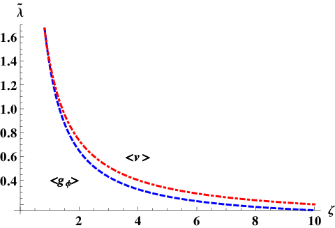
Figure 1 shows the dependency of $\braket{g_{\phi}}$ and $\braket{v}$ on the relativistic coldness $\zeta$, confirming the following limits for Eqs. (57):

It is also interesting to note that the maximum value of $\braket{g_{\phi}}$ is attained at $\zeta_{\rm max}\simeq 1.034$, where $\braket{g_{\phi}}\simeq 0.876$.

Using Eq. (56) for the definition of $\tau$, it is convenient to introduce the following notation:

where the “effective” transport coefficients $\widetilde{\eta}$, $\widetilde{\lambda}$ and $\widetilde{\mu}$ only depend on $\zeta_{E}$ (since $P_{E}=nm/\zeta_{E}$). Figure 2 shows a comparison of Eqs. (61) when the mean velocity is taken to be the average of the Möller velocity or the average of $v$, in terms of $\zeta$. It can be seen that, while $\widetilde{\lambda}$ and $\widetilde{\mu}$ decrease monotonically from infinite values at $\zeta\rightarrow 0$ to $0$ as $\zeta\rightarrow\infty$, the “effective”bulk viscosity $\widetilde{\eta}$ presents a maximum value at $\zeta=\zeta_{\rm max}$, while decreasing to $0$ as $\zeta\rightarrow 0$ or $\zeta\rightarrow\infty$. The value of $\zeta_{\rm max}$ depends on the definition of the mean velocity, having the value $\zeta_{\braket{g_{\phi}}}=1.342$ and $\zeta_{\braket{v}}=1.535$, when the mean velocity is taken as $\braket{g_{\phi}}$ and $\braket{v}$, respectively. A direct comparison of the curves for the transport coefficients corresponding to the relaxation time constructed using $\braket{g_{\phi}}$ and $\braket{v}$ reveals that their qualitative behaviour is the same in both cases. Thus, for the remainder of this paper, we will only discuss the case when $\braket{v}$ is employed.

To conclude this section, it is worth emphasizing that the tetrad formalism has made possible the analogy between the computation of the transport coefficients on curved spaces with respect to arbitrary coordinate systems and on Minkowski space in Cartesian coordinates. Moreover, the expressions (52), (54) and (55) for the coefficients of bulk viscosity, thermal conductivity and shear viscosity are identical to those obtained for Minkowski space [6], in agreement with Einstein’s equivalence principle. This is not surprising, since the equations (34) defining the transport coefficients, as well as Eq. (46) describing the non-equilibrium part of the stress-energy tensor, are written in a covariant form, reducing to the Minkowski expressions presented in Ref. [6] in the flat-space limit. The effect of curvature is however felt through the covariant derivatives in Eqs. (34), which define the transport coefficients. It is worth writing down the expression for $\nabla_{\hat{\gamma}}u^{\hat{\gamma}}$ appearing in Eq. (34a):

since, in the comoving frame, $u^{\hat{\gamma}}=(1,0,0,0)$.

We end this section by noting that the expressions that we obtained for the connection coefficients depend on the form of the constitutive equations. In this section, we defined the transport coefficients using Eqs. (34), which represent the covariant form of the standard definitions on Minkowski space [24]. While other definitions of the transport coefficients are possible [22, 23], in this paper we only consider the covariant formalism presented in this section.

Let us consider a central chart (i.e. static and spherically symmetric) whose metric in spherical coordinates $(x^{\mu})=(t,r,\theta,\varphi)$ may be written in the general form

where $u$, $v$ and $w$ depend only on the radial coordinate $r$. The non-vanishing Christoffel symbols corresponding to the above metric are given below (the prime denotes differentiation with respect to $r$):

For the remainder of this paper, we will consider rigidly rotating flows rotating with constant angular velocity $\Omega$ about the $z$ axis. The only non-vanishing components of the $4$-velocity of such flows are $u^{t}$ and $u^{\varphi}$, which can be found once $k^{\mu}=(k^{t},0,0,k^{\varphi})^{T}$ is known. Substituting $(\mu,\nu)=(t,r)$ in Eq. (30) gives:

where $C_{1}$ is an integration constant. Furthermore, setting $(\mu,\nu)=(r,\varphi)$ in Eq. (30) gives:

The function $\Theta(\theta)$ can be determined by setting $(\mu,\nu)=(\theta,\varphi)$:

where $C_{2}$ is an integration constant. Let us consider the norm of $k^{\mu}$:

where $\rho=r\sin\theta$ represents the distance to the $z$ axis. Since $k^{2}=-\beta^{2}$, it is convenient to set $C_{1}=-\beta_{0}$ and $C_{2}=\beta_{0}\Omega$, such that:

References

- [1] M. Casals, S. R. Dolan, B. C. Nolan, A. C. Ottewill, E. Winstanley, Phys. Rev. D 87 (2013) 064027.
- [2] A. Vilenkin, Phys. Lett. 80B (1978) 150.
- [3] A. Vilenkin, Phys. Rev. D 21 (1980) 2260.
- [4] J. R. Letaw, J. D. Pfautsch, Phys. Rev. D 22 (1980) 1345.
- [5] B. R. Iyer, Phys. Rev. D 26 (1982) 1900.
- [6] C. Cercignani, G. M. Kremer, The relativistic Boltzmann equation: theory and applications, Birkhäuser Verlag, Basel, Switzerland (2002).
- [7] G. Duffy, A. C. Ottewill, Phys. Rev. D 67 (2003) 044002.
- [8] F. Becattini, F. Piccinini, arXiv:0710.5694v2.
- [9] F. Becattini, L. Tinti, arXiv:0911.0864v4.
- [10] F. Becattini, Pisma v zchaia A 8 (2011) 13–19.
- [11] F. Becattini, L. Tinti, Phys. Rev. D 84 (2011) 025013.
- [12] F. Becattini, L. Tinti, Phys. Rev. D 87 (2013) 025029.
- [13] F. Becattini, L. Tinti, Int. J. Geom. Meth. Mod. Phys. 11 (2014) 1450020.
- [14]
V. E. Ambru
and E. Winstanley, Phys. Lett. B 734, 296 (2014).s , - [15] F. Becattini, E. Grossi, Phys. Rev. D 92, 045037 (2015).
- [16] D. Alba, H. W. Crater, L. Lusanna, Int. J. Geom. Meth. Mod. Phys. 12 (2015) 1550049.
- [17]
, R. Blaga, Annals of West University of Timisoara - Physics 58 (2015) 89.s , - [18] C. Marle, Annales de l’I.H.P. Physique théorique 10 (1969) 67.
- [19] R. W. Lindquist, Ann. Phys. (N. Y.) 37 (1966) 487.
- [20] H. Riffert, Astrophys. J. 310 (1986) 729.
- [21] C. Y. Cardall, E. Endeve, A. Mezzacappa, Phys. Rev. D 88 (2013) 023011.
- [22] G. M. Kremer, J. Stat. Mech. (2013) P04016; J. Stat. Mech. (2013) E05001; J. Stat. Mech. (2013) E10001.
- [23] G. M. Kremer, Int. J. Geom. Methods Mod. Phys. 11 (2014) 1460005.
- [24] L. Rezzolla, O. Zanotti, Relativistic hydrodynamics, Oxford University Press, Oxford, UK (2013).
- [25] W. K. Tung, Group theory in physics, World Scientific Publishing, Philadelphia, USA (1984).
- [26] C. W. Misner, K. S. Thorne, J. A. Wheeler, Gravitation, W. H. Freeman, San Francisco, USA (1973).
- [27] P. Romatschke, Phys. Rev. D 85 (2012) 065012.
- [28] W. Florkowski, E. Maksymiuk, Phys. G: Nucl. Part. Phys. 42 (2015) 045106.
- [29] W. Florkowski, Phenomenology of ultra-relativistic heavy-ion collisions, World Scientific, Singapore (2010).
- [30] J. L. Anderson, H. R. Witting, Physica 74 (1974) 489.
- [31] Y. Hatta, T. Kunihiro, Ann. Phys. 298 (2002) 24.
- [32] T. Kunihiro, K. Tsumura, J. Phys. A 39 (2006) 8089.
- [33] T. Tsumura, T. Kunihiro, K. Ohnishi, Phys. Lett. B 646 (2007) 134.
- [34] J. L. Anderson, H. R. Witting, Physica 74 (1974) 466.
- [35] M. Abramowitz, I. A. Stegun, Handbook of mathematical functions (National Bureau of Standards, Washington, 1972).
- [36] F. W. J. Olver, D. W. Lozier, R. F. Boisvert, C. W. Clark, NIST handbook of mathematical functions (Cambridge University Press, New York, 2010).
- [37] R. C. Tolman, Phys. Rev. 35 (1930) 904.
- [38] R. C. Tolman, P. Ehrenfest, Phys. Rev. 36 (1930) 1791.
- [39] G. Pascu, Atlas of Coordinate Charts on the de Sitter Spacetime, arXiv:1211.2363v1 [gr-qc] (2012).
- [40] N. Nicolaevici, Classical Quantum Gravity 18 (2001) 5407.
- [41]
, E. Winstanley, AIP Conf. Proc. 1634 (2014) 40.s , - [42]
, in preparation.s ,