The dynamics of clusters of galaxies from the GCLASS survey
Abstract
Context. The dynamics of clusters of galaxies and its evolution provide information on their formation and growth, on the nature of dark matter and on the evolution of the baryonic components. Poor observational constraints exist so far on the dynamics of clusters at redshift .
Aims. We aim to constrain the internal dynamics of clusters of galaxies at redshift , namely their mass profile , velocity anisotropy profile , and pseudo-phase-space density profiles and , obtained from the ratio between the mass density profile and the third power of the (total and, respectively, radial) velocity dispersion profiles of cluster galaxies.
Methods. We use the spectroscopic and photometric data-set of 10 clusters at from the Gemini Cluster Astrophysics Spectroscopic Survey (GCLASS). We determine the individual cluster masses from their velocity dispersions, then stack the clusters in projected phase-space. We investigate the internal dynamics of this stack cluster, using the spatial and velocity distribution of its member galaxies. We determine the stack cluster using the MAMPOSSt method of Mamon et al., and its by direct inversion of the Jeans equation. The procedures used to determine the two aforementioned profiles also allow us to determine and .
Results. Several models are statistically acceptable for the stack cluster (Burkert, Einasto, Hernquist, NFW). The stack cluster total mass concentration, , is in agreement with theoretical expectations. The total mass distribution is less concentrated than both the cluster stellar-mass and the cluster galaxies distributions. The stack cluster indicates that galaxy orbits are isotropic near the cluster center and become increasingly radially elongated with increasing cluster-centric distance. Passive and star-forming galaxies have similar . The observed is similar to that of dark matter particles in simulated cosmological halos. and are almost power-law relations with slopes similar to those predicted from numerical simulations of dark matter halos.
Conclusions. Comparing our results with those obtained for lower-redshift clusters, we conclude that the evolution of the concentration-total mass relation and pseudo-phase-space density profiles agree with the expectations from CDM cosmological simulations. The fact that and already follow the theoretical expectations in clusters suggest these profiles are the result of rapid dynamical relaxation processes, such as violent relaxation. The different concentrations of the total and stellar mass distribution, and their subsequent evolution, can be explained by merging processes of central galaxies leading to the formation of the BCG. The orbits of passive cluster galaxies appear to become more isotropic with time, while those of star-forming galaxies do not evolve, presumably because star-formation is quenched on a shorter timescale than that required for orbital isotropization.
Key Words.
Galaxies: clusters: general; Galaxies: kinematics and dynamics1 Introduction
The total mass density profiles () of cosmological halos are known to be well described by universal profiles such as the NFW profile of Navarro et al. (1996); Navarro et al. (1997) and the profile of Einasto (1965, see also ), at least in the radial range from 10 kpc (Schaller et al. 2015) to the virial radius11 1 The radius is the radius of a sphere with mass overdensity times the critical density at the cluster redshift. Throughout this paper we refer to the radius as the ’virial radius’, . Given the cosmological model, the virial mass follows directly from once the cluster redshift is known, , where is the Hubble constant at the mean cluster redshift. The virial velocity is related to the virial radius by , (Diemer & Kravtsov 2014). This has been confirmed observationally in the local Universe, in particular on the scale of clusters of galaxies (Carlberg et al. 1997a; van der Marel et al. 2000; Biviano & Girardi 2003; Kneib et al. 2003; Arnaud et al. 2005; Biviano et al. 2013, e.g.). It is important to characterize the shape of the halo mass density profiles since they carry information on the nature of the matter contained in cosmological halos as well as on the way these halos form and evolve.
In general, the NFW and/or Einasto profiles are thought to result from an initial, fast assembly of halos (Huss et al. 1999; El-Zant 2008; Lapi & Cavaliere 2011, e.g.), where the dominant dynamical process are those of chaotic mixing and violent relaxation (Hénon 1964; Lynden-Bell 1967). These profiles are characterized by a scale radius and a smoothly changing slope with radius. On the other hand, the pseudo-phase-space density profile, , where is the total velocity dispersion profile of dark matter (DM) particles, has a simple power-law behavior, , over a wide radial range (Del Popolo 2011, outside 0.1% of the virial radius;) with a universal value of for a variety of cosmological halos (Taylor & Navarro 2001; Dehnen & McLaughlin 2005; Knollmann et al. 2008, e.g.). For this reason, Taylor & Navarro (2001) have argued that is a more fundamental dynamical quantity than . A similar power-law behavior (with a slightly different slope, ) also characterizes the related quantity (Dehnen & McLaughlin 2005), where is the radial component of .
The origin of the power-law behavior of and is not completely understood. It has been shown analytically (Dehnen & McLaughlin 2005) that it can result from the Jeans equation if a linear relation exists between the logarithmic slope of , , and the velocity anisotropy profile
| (1) |
where , , and are the radial, and the two tangential components, respectively, of the velocity dispersion, and where is usually assumed. A possible explanation of why there should be a linear relation between and has been proposed by Hansen (2009) in terms of the relative shapes of the radial and tangential velocity distribution functions of bound particles in a halo. In summary, it appears that the power-law behavior of and can be explained as the result of violent relaxation followed by dynamical equilibrium in a static gravitational potential.
The value of the power-law radial slope of seems to depend on the cosmological model in which the halos evolve (Knollmann et al. 2008), as well as on redshift () because is related to the halo mass and the halo growth-rate (Lapi & Cavaliere 2009). Lapi & Cavaliere (2009) predict the power-law exponent of to change by % over the range . Studying how evolves with redshift could therefore help us understand the processes of formation and evolution of cosmological halos.
Currently, little is known observationally about the (and ) of clusters. One of the quantities entering , namely , can be determined by several techniques, e.g. via gravitational lensing, cluster kinematics, and the emission from the hot intra-cluster medium. The other quantity, ( in the case of ), cannot be determined observationally for DM particles, but it can be derived for cluster galaxies, assuming that their velocity distribution is the same as that of DM particles. This requires a large spectroscopic sample of cluster members.
Munari et al. (2014) determined and for a cluster, and found it to be consistent with a power-law behavior, although with more negative exponents than found in numerical simulations ( vs. and vs. ). Biviano et al. (2013) determined and for a cluster from the CLASH-VLT survey (Rosati et al. 2014) and found consistency with the theoretically predicted power-law behavior, although Fig. 17 in their paper suggests slightly less negative exponents than the theoretical expectations. It is clearly impossible to draw conclusions based on only two clusters, but the observed redshift trend of appears to go in the opposite sense to the theoretical expectation by Lapi & Cavaliere (2009).
Strictly related to the determination of and is the determination of the velocity anisotropy profile . Mahdavi et al. (1999); Biviano & Katgert (2004); Hwang & Lee (2008); Munari et al. (2014) have found that in low-redshift () groups and clusters for non-emission-line/early-type/red galaxies (hereafter generically referred to as ’PG’ for passive galaxies), while for emission-line/late-type/blue galaxies (hereafter generically referred to as ’SFG’ for star-forming galaxies). In other words, PG are characterized by mostly isotropic orbits (van der Marel et al. 2000; Katgert et al. 2004, see also), while SFG are characterized by increasingly radially elongated orbits with distance from the cluster center (which we refer to as ’radius’ hereafter). At higher redshifts, () cluster galaxy orbits appear to be more similar across different galaxy types (Biviano & Poggianti 2009; Biviano et al. 2013), and increasingly radially elongated with radius. This suggests that the orbits of PG become more isotropic with time, while those of SFG do not evolve.
More clusters are becoming available for the determination of and , both at low-, from the WINGS (Cava et al. 2009) and its extension OmegaWINGS (Gullieuszik et al. 2015), and at intermediate-, from the CLASH-VLT survey (Rosati et al. 2014). At higher all the analyses so far have been limited to the determination of , generally modeled with an NFW or an isothermal sphere profile. Sereno & Covone (2013) collected data for 30 clusters at , and derived their concentrations and virial masses from strong and weak lensing analyses, assuming an NFW . The compilation of Sereno & Covone (2013) include all known clusters for which has been derived so far, except for “El Gordo”, whose mass profile has been determined via gravitational lensing by Jee et al. (2014). The mass profiles of some clusters in the compilation of Sereno & Covone (2013) have been determined in more than one study, generally by gravitational lensing techniques (Clowe et al. 2000; Jee et al. 2005a; Jee et al. 2005b; Lombardi et al. 2005; Jee et al. 2006; Jee & Tyson 2009; Jee et al. 2009), and in some cases by using hydrostatic equilibrium equations based on X-ray data (Huo et al. 2004; Santos et al. 2012) and/or the thermal SZ effect (Adam et al. 2015). In none of these studies have or been determined.
In this paper we use the sample of high- clusters from GCLASS (Muzzin et al. 2012) to investigate their dynamics. We use the kinematics of cluster members to determine , , , and of a stacked sample of 418 cluster members, belonging to 10 clusters at . The structure of this paper is the following. In Sect. 2 we describe our data-set, the selection of cluster member galaxies, and the stacking procedure. In the following Sections, we determine (Sect. 3), (Sect. 4), and (Sect. 5), of the stack cluster. We discuss our results in Sect. 6 and summarize them and draw our conclusions in Sect. 7. Throughout the paper we adopt km s-1 Mpc-1, , .
2 The sample
2.1 The data-set
The GCLASS sample consists of 10 rich clusters at , and is fully described in Muzzin et al. (2012). These clusters were selected using the red-sequence method (Gladders & Yee 2000) from the SpARCS survey (Muzzin et al. 2009; Wilson et al. 2009). The photometric catalog is described in van der Burg et al. (2013) and it is complete down to a median stellar mass limit of (van der Burg et al. 2014, vdB14 hereafter). Spectroscopic coverage was obtained through observations on the GMOS instruments on the Gemini North and Gemini South telescopes. Spectroscopic targets were chosen upon prioritization by three criteria, a) clustercentric distance, b) observed m color, and c) m flux, in order of importance, see Muzzin et al. (2012). The number of galaxies with measured within the fields of the 10 clusters vary between 49 and 162 (Muzzin et al. 2012), with an average22 2 Here and throughout this paper, we adopt the biweight estimation of central location for the average, and the biweight estimation of scale for the dispersion of a given statistical set (Beers et al. 1990). of 137. The total number of cluster members in each field is a subset of these redshifts. In Table 1 we list the cluster names, the total number of redshifts for galaxies in the field of each cluster, the number of cluster members (identified as described in Sect. 2.2), their mean spectroscopic redshift and line-of-sight velocity dispersion , and the clusters determined from as described in Sect. 2.2. The coordinates of the cluster centers are given in 98 Table 1, and are based on the positions of the Brightest Cluster Galaxies (BCG), determined by Lidman et al. (2012).
| SpARCS | |||||
|---|---|---|---|---|---|
| number | [] | [kpc] | |||
| 0034 | 137 | 40 | 0.866 | ||
| 0035 | 49 | 21 | 1.336 | ||
| 0036 | 119 | 48 | 0.869 | ||
| 0215 | 125 | 46 | 1.004 | ||
| 1047 | 147 | 29 | 0.956 | ||
| 1051 | 145 | 32 | 1.034 | ||
| 1613 | 161 | 83 | 0.872 | ||
| 1616 | 162 | 43 | 1.155 | ||
| 1634 | 125 | 48 | 1.177 | ||
| 1638 | 112 | 38 | 1.195 |
2.2 Cluster membership
Muzzin et al. (2012) established the cluster membership of galaxies with in a simple way, by requiring member galaxies to lie within 1500 of the mean cluster velocity in rest-frame. Their definition was sufficiently accurate for their purposes. The study of the internal cluster dynamics requires however a more accurate membership determination. We proceed as follows. First, we split the distribution of each cluster into groups separated by weighted gaps with value (see Beers et al. 1991, for the definition of ’weighted gap’), and we select the richest of these groups. Then, we apply three algorithms for the definition of cluster membership, those of den Hartog & Katgert (1996), Fadda et al. (1996, ’shifting gapper’), and Mamon et al. (2013, ’Clean’). All these use the location of galaxies in projected phase-space , where is the projected radial distance from the cluster center, is the rest-frame velocity and is the mean cluster redshift. For the ’shifting gapper’ method we adopt the following parameters: 600 kpc for the bin size, a minimum of 15 galaxies per bin, and 800 for the significance of the gap in velocity space (see Fadda et al. 1996, for details on the meaning of these parameters). If a galaxy passes the membership criteria of at least three of the four algorithms considered (Muzzin et al. 2012, including that of), it is considered as a bona fide cluster member. The resulting number of cluster members is listed in Table 1.
Based on the sample of cluster members, we compute the line-of-sight velocity dispersion, , of each cluster. This is corrected for the errors in measured , which are typically , according to Danese et al. (1980). To obtain an estimate of the cluster virial radius, , from we follow the iterative procedure of Mamon et al. (2013). This assumes an NFW model for the mass distribution, the concentration–mass relation of Gao et al. (2008), and the model of Mamon & Łokas (2005) for the velocity anisotropy profile, with the same scale radius as that of the mass profile (Mamon et al. 2010, as suggested by). Using different concentration–mass relations and velocity anisotropy profiles within currently accepted models in the literature does not modify the resulting values in a significant way.
2.3 Stacking the clusters
The number of spectroscopic members is too low in any individual cluster of our sample to allow determination of its mass profile by the analysis of kinematics (see Table 1). We therefore stack the individual clusters together, under the assumption that their mass profiles have a similar shape and differ only by their normalization. This is a widely used procedure (van der Marel et al. 2000; Rines et al. 2003; Katgert et al. 2004, e.g.) and it relies on the predicted existence of a universal mass profile for cosmological halos (Navarro et al. 1997), and the fact that the concentration of halo mass profiles is only mildly dependent on their mass (Gao et al. 2008; Macciò et al. 2008; De Boni et al. 2013; Groener et al. 2016, e.g.). The concentration of a halo mass profile can be defined as where is the radius at which . In our sample, given the and values that we have determined, we expect a very narrow range in concentration, –3.2, following the relation of De Boni et al. (2013).
The stacking is done in projected phase-space after scaling the cluster-centric distances by the cluster , , and the line-of-sight rest-frame velocities by the cluster , .
We define the properties of the stack cluster by the weighted average of the properties characterizing its component clusters, using the number of cluster members as weights. The stack cluster has a mean redshift , and a virial radius kpc, corresponding to a virial mass . Since the stack was built by centering the clusters on the positions of their BCGs, these 10 galaxies are removed from the stack in all the following analyses. After removing the BCGs, the stack cluster contains 418 member galaxies, of which 355 are at , 273 are PG, 123 are SFG, and the rest do not have a type classification44 4 The type classification is based on the and rest-frame colors (98)..

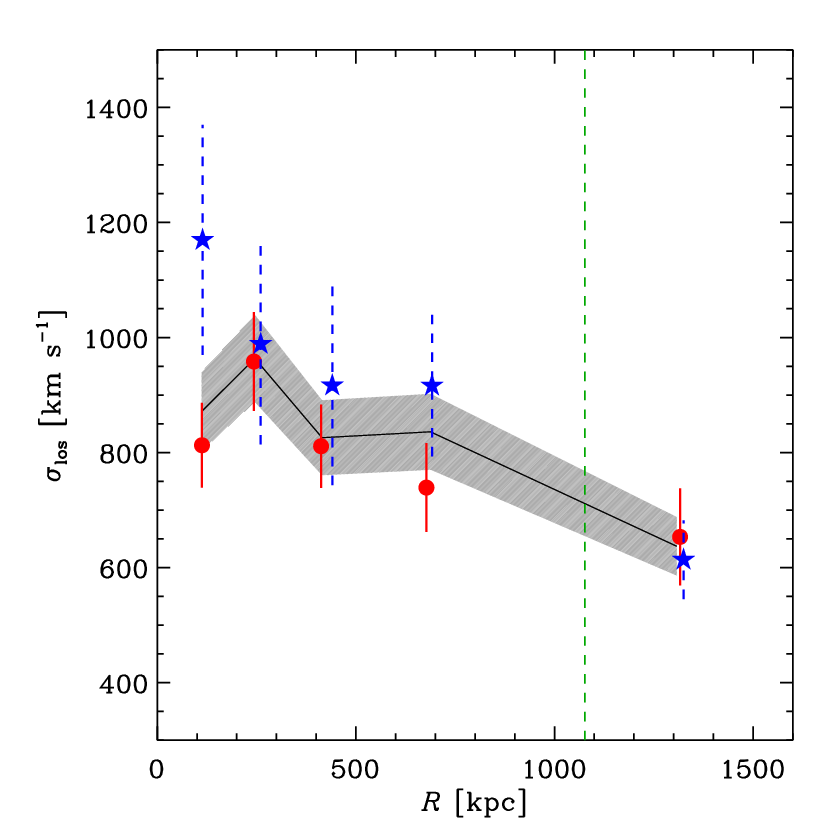
The projected phase-space distribution of PG and SFG in the stack cluster is shown in Fig. 1 (Muzzin et al. 2014, see also). In Fig. 2 we show the line-of-sight velocity dispersion profiles of the stack cluster, evaluated on all galaxies, and also, separately, on PG and SFG. It has been shown by 98 that the number density profiles of PG and SFG in the GCLASS sample are significantly different. We confirm this difference by a Kolmogorov-Smirnov test (Press et al. 1992, e.g.), which returns a probability of that the radial distributions of PG and SFG are drawn from the same parent population. On the other hand, the same test applied to the distributions of rest-frame velocities does not reject the null hypothesis that the two distributions are drawn from the same parent one. This is confirmed by the similar of PG and SFG, shown in Fig. 2. There is however a systematic difference between the two , in that SFG have larger than PG within . The ratios of the SFG to the PG is 0.69, 0.97, 0.88, 0.81, and 1.06 in the 5 radial bins shown in Fig. 2. Similar differences are seen in the of SFG and PG of nearby (Biviano et al. 1997, see, e.g., Fig. 13 in) and medium-distant (Carlberg et al. 1997b, see, e.g., Fig. 2 in) clusters.
3 The mass profile
We use the MAMPOSSt technique (Mamon et al. 2013) to determine the mass profile of the stack cluster (described in Sect. 2.3). MAMPOSSt performs a maximum likelihood analysis of the distribution of cluster galaxies in projected phase-space, comparing it with theoretical distributions predicted by the Jeans equation (Binney & Tremaine 1987) for given models of the mass and velocity anisotropy profiles. It has been tested on cluster-size halos extracted from cosmological simulations (Mamon et al. 2013) and applied to several galaxy clusters already (Biviano et al. 2013; Guennou et al. 2014; Munari et al. 2014; Durret et al. 2015; Balestra et al. 2016; Pizzuti et al. 2016).
The spatial distribution of galaxies in a stack of the same clusters used in this paper has already been fitted by 98. We here repeat their analysis to take into account the fact that our values of the clusters are different from theirs. We find that the number density profile of all galaxies members of the stack is best-fitted by an NFW profile with concentration , a value identical to that found by 98.
Having fitted the spatial distribution of galaxies, we can restrict the MAMPOSSt maximum likelihood analysis to the velocity distribution of cluster galaxies. This is the so-called ’Split’ case of the MAMPOSSt procedure (Mamon et al. 2013).
| Velocity | Likelihood | |||
|---|---|---|---|---|
| models | [Mpc] | Anisotropy | ratio | |
| Bur | C | 0.32 | ||
| Bur | O | 1.00 | ||
| Bur | T | 0.60 | ||
| Ein | C | 0.10 | ||
| Ein | O | 0.36 | ||
| Ein | T | 0.21 | ||
| Her | C | 0.13 | ||
| Her | O | 0.52 | ||
| Her | T | 0.29 | ||
| NFW | C | 0.13 | ||
| NFW | O | 0.41 | ||
| NFW | T | 0.24 | ||

We consider the four following models for :
- 1.
- 2.
the model of Einasto (1965),
(3) ’Ein’ model hereafter, where is the regularized incomplete gamma function. We fix , a typical value for cluster-size halos extracted from cosmological numerical simulations (Mamon et al. 2010). The model is characterized by a slope approaching zero near the center, .
- 3.
The model of Hernquist (1990),
(4) ’Her’ model hereafter, where . It is characterized by , like the NFW model, and by a steeper asymptotic slope .
- 4.
The model of Burkert (1995),
(5) ’Bur’ model hereafter, where . The model is characterized by its central core, and an asymptotic slope like NFW, .
All models are characterized by just two parameters, and a scale radius, namely for the Ein and NFW models, and for the Her and Bur models, respectively. However, the stack cluster has a fixed value of by construction (see Sect. 2.3), and so the only remaining free parameter is the scale radius.
As for the velocity anisotropy profiles, we consider three models. The first, named ’C’, is , i.e. the velocity anisotropy is constant at all radii. The second, named ’O’ (for opposite) is characterized by opposite values of the velocity anisotropy at the cluster center and at very large radii, and it has been introduced by Biviano et al. (2013),
| (6) |
with . The third, named ’T’, is a simplified version of the model of Tiret et al. (2007), that has been shown to fit rather well the of cluster-sized halos extracted from numerical simulations (Mamon et al. 2010; Mamon et al. 2013),
| (7) |
with . In the T model, grows from central isotropy to increasingly radial velocity anisotropy at larger radii. It coincides with the model of Mamon & Łokas (2005) when and the scale radius of the Mamon & Łokas (2005) model coincides with .
All three models contribute only one additional free parameter to the MAMPOSSt analysis, i.e. or , since in the O and T models is forced to be the same parameter of .
We run MAMPOSSt on the 355 members of the stack cluster at . The results of the MAMPOSSt analysis are given in Table 2. The errors on each of the two free parameters of the analysis, and the velocity anisotropy parameter, are obtained after marginalizing on the other parameter. Note that instead of listing the values of the and velocity anisotropy parameters we list the values of the related parameters and , respectively (note that corresponds to , see eq.(1)). In Fig. 3, we show the best-fit results of MAMPOSSt within their 1 confidence contours in the plane of the velocity anisotropy parameter (, constant at all radii for the C model, and evaluated at for the O and T models) vs. . The value of is the same for all models, being fixed at the value obtained for the stack cluster in Sect. 2.3. Both in the Table and in the Figure we use the factors of 1/2 and 3/2 to convert the scale radii of the Her, and, respectively, the Bur to values.
In Table 2 we also list the likelihood ratio with respect to the maximum obtained among the twelve model combinations. Formally, the best-fit model combination is Bur+O, but all other combinations are statistically acceptable. This means that we are unable to distinguish the quality of different model fits with the present data-set. This is also clear from Fig. 3, where the best-fit solutions for the different models are all within 1 . C models have however systematically lower likelihoods than O and T models, and best-fit values of are always positive, suggesting that a radially increasing velocity anisotropy is a better fit to the data than a constant velocity anisotropy.

We estimate the weighted average of all values, using the relative likelihoods of the different models as weights. We find Mpc, where the error represents the weighted dispersion of the different model values. The uncertainties on the values of the individual models (see Table 2) are much larger than the dispersion in the best-fit values among different models (see also Fig. 3). In Fig. 4 we display the vs. theoretical relations of Bhattacharya et al. (2013, within its theoretically predicted scatter) and De Boni et al. (2013), and the value obtained for our stack cluster. We also display the phenomenological relation of Groener et al. (2016), which is based on 293 clusters and a variety of observational techniques (lensing, X-ray, kinematics). All relations are evaluated at the redshift of our stack cluster, . The value is taken from Sect. 2.3; the value is derived from the value of Sect. 2.3 and either the value of the best-fit MAMPOSSt model (Bur+O; , indicated by the red dot) or that obtained by taking the average of the of all twelve models, weighted according to their relative likelihoods (, indicated by the black diamond). The uncertainties in the values of and have been propagated to the uncertainty. We find that the stack cluster has a concentration in agreement within 1 with the observational relation of Groener et al. (2016), and also close to both the theoretical relations of De Boni et al. (2013) and Bhattacharya et al. (2013), especially when considering the large theoretically expected scatter.
4 The velocity anisotropy profile
The MAMPOSSt analysis has already provided us with best-fit values for the parameters of three models. Here we derive in a non-parametric way, without assuming a model shape for , by direct inversion of the Jeans equation, a problem first solved by Binney & Mamon (1982). In our analysis we follow the procedures of Solanes & Salvador-Solé (1990) and Dejonghe & Merritt (1992, the latter serving as a check for the former in our analysis). We use the same number density profile parametrization used for the MAMPOSSt procedure in Sect. 3. We then derive a binned line-of-sight velocity dispersion profile (see Fig. 2) and smooth it with the LOWESS technique (Gebhardt et al. 1994, see, e.g.,), linearly extrapolated to infinity (in practice, 30 Mpc from the cluster center) to a value of 20% its peak value (we checked that the details of this extrapolation are irrelevant for our solution within ). For the Jeans equation inversion we adopt the maximum-likelihood from MAMPOSSt (the Bur model of the second line of Table 2).

To determine the uncertainties in we run 50 bootstrap resamplings of the galaxies that define the velocity dispersion profile in the stack cluster, and for each of these resamplings we run 20 random choices of the value of the LOWESS smoothing parameter. The uncertainties of are estimated as the upper and lower quartiles of the bootstrap determinations with respect to the median. We find that the uncertainties in are dominated by the statistics, and not by the systematics in the smoothing procedure.
In Fig. 5 (top panel) we show the solution and its 68% confidence levels. Galaxy orbits are close to isotropic near the center and become more radially elongated at larger cluster-centric distances. Using the best-fit solutions for other models (Ein, Her, NFW) (see Table 2) in the Jeans equation inversion, does not change in a significant way (i.e. the profiles remain well within the 68% confidence region shown in Fig. 5), independently on which model was assumed in the MAMPOSSt analysis.
In Fig. 5 (top panel) we also display the maximum-likelihood O solution found by MAMPOSSt (second line of Table 2). This is in good agreement with the solution obtained by inversion of the Jeans equation, indicating that the adopted O model is a good one. On the other hand, the C model (albeit still acceptable) cannot reproduce the increasing anisotropy with radius, and this is consistent with the fact that the likelihoods obtained by MAMPOSSt are systematically lower for the C models than for the O (and T) models.
We also consider PG and SFG separately, by adopting the same best-fit Bur model from MAMPOSSt (since the cluster gravitational potential is the same for any tracer), but different number density and velocity dispersion profiles. The number density profiles have been determined separately for the two classes of galaxies, by following the procedure of 98, and are best-fitted by NFW models with concentrations and , respectively (98, these values are very close to those found by). The velocity dispersion profiles for the two galaxy populations have already been derived in Sect. 2.3 and are displayed in Fig. 2. The bottom panel of Fig. 5 shows that PG and SFG are characterized by very similar , and hence, orbits, within the stack cluster.
5 The pseudo-phase-space density profiles

Using the determination of (and therefore ) from MAMPOSSt (in Sect. 3) and of (Solanes & Salvador-Solé 1990, and therefore and , see eqs. 20 and 21 in) from the direct inversion of the Jeans equation (in Sect. 4), we determine and . Their uncertainties are derived from the propagation of the errors on and . The errors on comes from the MAMPOSSt analysis, while those on and are a byproduct of the bootstrap procedure used to determine the errors on .
In Fig. 6 we show the resulting profiles and their 68% confidence regions. These profiles are based on the maximum-likelihood MAMPOSSt model (second line of Table 2). Other MAMPOSSt best-fit results based on the T model and Ein, Her, or NFW give very similar and , well within the uncertainties, and are not displayed in Fig. 6 for the sake of clarity. We have not considered the C models, as these were shown to be less likely (see Sect. 3 and 4).
In the same figure we also display the theoretical power-law relations and with from Dehnen & McLaughlin (2005), based on halos from cosmological, DM-only simulations, as well as the relation with , valid for massive halos at (Lapi & Cavaliere 2009, see Fig. 6 in). The normalizations of these relations are fitted to the data in the figure. The observed and profiles are very close to the theoretical power-law relations and consistent with them within the 1 uncertainties over the full radial range out to .
6 Discussion
We have investigated the dynamics of a stack of 10 rich clusters from GCLASS (Muzzin et al. 2012), at mean redshift and with mean (inferred from ) mass . To infer the mass and velocity-anisotropy profiles, and , we have applied the MAMPOSSt technique of Mamon et al. (2013), and the Jeans inversion procedure of Solanes & Salvador-Solé (1990). Hereafter we discuss our results for and .
6.1 The mass profile
We find that we are unable to discriminate among different models characterized by different inner and asymptotic slopes (see eqs. 2, 3, 4, 5). Independently of the model considered, the concentration of the mass profile, , is only slightly above (but not significantly different from) the theoretical expectations by Bhattacharya et al. (2013) and De Boni et al. (2013) for a cluster of the same mass and at same redshift as our stacked cluster (see Fig. 4). It is also consistent, albeit slightly below, the observational relation of Groener et al. (2016) which is based on a heterogeneous sample of 293 clusters and derived using different techniques (lensing, X-ray, kinematics).
| range | Ref | Note | ||
|---|---|---|---|---|
| Total mass | ||||
| 0.02-0.13 | 0.7 | BG03 | S43 | |
| 0.04-0.08 | 6.1 | KBM04 | S59 | |
| 0.17-0.55 | 8.2 | vdM+00 | S16 | |
| 0.19-0.35 | 13.1 | Mer+15 | A9 | |
| 0.36-0.54 | 10.2 | Mer+15 | A8 | |
| 0.39-0.79 | 2.8 | BP09 | S19 | |
| 0.69-0.89 | 1.1 | Mer+15 | A2 | |
| 0.78-1.46 | 4.1 | SC13 | S31 | |
| 0.87-1.33 | 4.5 | This paper | S10 | |
| Stellar mass | ||||
| 0.01-0.09 | 2.0 | LMS04 | S93 | |
| 0.04-0.11 | 5.0 | vdB+15 | S31 | |
| 0.11-0.25 | 5.0 | vdB+15 | S30 | |
| 0.19-0.55 | 12.0 | Muz+07 | S15 | |
| 0.44-0.44 | 14.0 | Ann+14 | 1 | |
| 0.87-1.33 | 4.5 | This paper | S10 | |

The concentration of the total cluster mass is not significantly different from that of the distribution of cluster galaxies (), while both are significantly less concentrated than the stellar-mass distribution, . We determine this value by applying the procedure of 98 using our scalings (see Sect. 3). The value we determine is only slightly different from that of 98.
In van der Burg et al. (2015) the concentration of the stellar mass distribution was shown to evolve from in the GCLASS sample to in a sample of clusters with masses that would make them the likely descendants of the GCLASS clusters in a hierarchical CDM cosmology. The low- and intermediate- data used in van der Burg et al. (2015) are shown in Fig. 7, right panel, with the addition of one data point from Annunziatella et al. (2014). The values shown in the figure are reported in Table 3. In the same figure we also show the theoretical concentration vs. relations for clusters of different masses, obtained for DM-only cosmological simulations by Bhattacharya et al. (2013) and for hydrodynamical cosmological simulations by De Boni et al. (2013). Clearly, the evolution observed in is much stronger, and in the opposite sense, of the evolution expected for the total mass distribution.
| Concentration | Model | ||
|---|---|---|---|
| total mass () | Bha13 | 10 | 12.8 |
| total mass () | DeB13 | 10 | 19.7 |
| stellar mass () | Bha13 | 6 | 118.1 |
| stellar mass () | DeB13 | 6 | 51.1 |
In the left panel of Fig. 7 we compare the theoretical expectations to the concentrations derived for the total mass distributions in clusters of different masses and at different , using the result of this paper and a compilation of values from the literature (see Table 3). The agreement is much better than found for the stellar mass concentrations. We quantify this (dis)agreement by the quantity
| (8) |
where are the observed concentrations for the total or stellar mass, are their uncertainties, and are the expected concentrations for halos of the same masses and , from either Bhattacharya et al. (2013) or De Boni et al. (2013). The values are given in Table 4. The model of Bhattacharya et al. (2013) is an acceptable description of the observed total mass concentrations as a function of , at the 17% confidence level. The model of De Boni et al. (2013) is also marginally acceptable (2% confidence level), while the observations cannot be described by any of the two models.
Neither in the total nor in the stellar mass density profile have the BCGs been considered. As pointed out by van der Burg et al. (2015), the strong observed evolution of could be due to the build-up of the BCG via merger of central galaxies. Lidman et al. (2012) have found that BCGs grow on average by a factor in stellar mass between and , mostly via dry mergers. About half of this growth is due to major mergers (Lidman et al. 2013). The so-called Spiderweb galaxy (Miley et al. 2006) is a famous high- example of a forming BCG. In the merging process part of the stellar mass may also get dispersed into the intra-cluster light component (Annunziatella et al. 2014; Annunziatella et al. 2016, see, e.g.), which has also not been accounted for, in our stellar mass density profile determination.
Galaxies present in the central region of clusters make the stellar mass density profile very concentrated. As they merge to form the central BCG, the stellar mass density profile flattens at the center, if the contribution of the BCG itself is not accounted for, and if the merged galaxies are not replaced. The reason why the merged galaxies are not replaced in lower- clusters is possibly due to the increasing timescale for dynamical friction, as the cluster grows more massive with time (van der Burg et al. 2015).
6.2 The pseudo-phase-space density profiles
Similarly to , also the pseudo-phase-space density profiles follow closely the theoretical predictions, namely the power-laws of Dehnen & McLaughlin (2005), at any redshift at which they have been estimated so far (Biviano et al. 2013; Munari et al. 2014), including the present study. However, the and power-law slopes of our stack cluster are % more negative than the theoretically expected ones of Dehnen & McLaughlin (2005). Since the latter were derived for halos, the slight difference might hint to an evolution of the pseudo-phase-space density profiles.
Such an evolution has indeed been predicted by Lapi & Cavaliere (2009). They relate with the dynamical entropy of the system, , itself regulated by the mass and the mass accretion rate of the system, . Since evolves with , so does the power-law slope of , . The expected evolution over the redshift range from to 1 is only 10%. Lapi & Cavaliere (2009) predict for at (see their Fig. 6), in perfect agreement with the observed slope of the of our stack cluster. Given the large observational uncertainties, such a perfect agreement must be considered a coincidence, and more data are needed to really constrain as a function of .
A note of caution is that we are here comparing profiles obtained for the DM component in simulations, with profiles obtained using the total mass density profile () and the total () or radial () velocity dispersion profiles of cluster galaxies. So the comparison of the observed and with the theoretically predicted ones is not fully straightforward, and it could be affected by any velocity bias between the cluster galaxy and DM particle components (Biviano et al. 2006, see, e.g.). As long as this velocity bias does not depend on the radius, however, only the normalization of and would be affected and not the power-law slope, which is the quantity we are interested in here. Turning this argument around, the good agreement between the theoretical and observed slopes suggests that any scale-dependent velocity bias between the DM and galaxy components of galaxy clusters must be small, and this is perhaps not too surprising given that they are both nearly collisionless components.
Overall, the consistency of the and observed evolution with the theoretical expectations suggest that our current understanding of the evolution of the DM component of massive halos is correct. It indicates that GCLASS clusters are dynamically evolved systems. Given that no well-formed cluster has so far been observed at (Newman et al. 2014), this leaves Gyr for clusters to reach dynamical equilibrium after their initial assembly. Such a short time suggests that the origin of the power-law behavior of (and its universality) is violent relaxation (Lynden-Bell 1967).
6.3 The velocity anisotropy profiles
The of our clusters is very similar to that predicted for DM particles in cluster-size halos from numerical simulations (Mamon et al. 2010; Munari et al. 2013, e.g.), namely nearly isotropic near the cluster center and increasingly elongated with radius. This shape is as predicted for a cosmological halo evolving through an initial phase of fast collapse and a subsequent slow phase of inside-out growth by accretion of field material (Lapi & Cavaliere 2011). The cluster is also similar to the found for cluster galaxies at intermediate- (Biviano & Poggianti 2009; Biviano et al. 2013; Annunziatella et al. 2016). Both at and at intermediate- PG and SFG have similar . Given that the PG population grows from the quenching of SFG, the observed similarity of the orbits of these two classes of galaxies at intermediate- and high- is not surprising. At low-, however, the orbits of SFG and PG become different, as PG develop nearly isotropic orbits at all radii out to , while the orbits of SFG do not change (Mahdavi et al. 1999; van der Marel et al. 2000; Biviano & Katgert 2004; Katgert et al. 2004; Biviano & Poggianti 2009; Munari et al. 2014).
Observations suggest that the evolution of PG orbits happens at , i.e. in the last Gyr of cosmic time. Before that, orbital evolution processes might be masked by the continuous replenishement of the cluster population by recently infallen galaxies. These are SFG that will have their star-formation quenched by the cluster environment, or galaxies that are already passive when they enter the cluster (Balogh et al. 2000, ’pre-processing’; see). Only when the mass accretion rate declines significantly, and the cluster PG population is mostly frozen, its orbital distribution can evolve. The Gyr timescale for orbital evolution then sets an upper limit to the quenching timescale, or we would be able to observe a similar orbital evolution for the SFG population.
There are several processes that could in principle cause orbital isotropization, such as dynamical friction, violent relaxation following major mass accretion by the clusters, modification of the gravitational potential by secular mass accretion (Gill et al. 2004), radial orbital instability (Bellovary et al. 2008), and interaction with the intra-cluster medium (Dolag et al. 2009). Insight in which of these processes is more effective in shaping galaxy orbits can come from an estimate of their relative timescales at different epochs of the cluster evolution.
Numerical simulations can be very useful in this context. So far they have succeeded in reproducing the overall shape of the of cluster galaxies, but unfortunately they have produced discordant results on its evolution. Some simulations predict marginal isotropization of the orbits of galaxies (or DM particles) with time (Wetzel 2011; Munari et al. 2013), at least in qualitative agreement with the observed evolution, while others predict no evolution at all or an evolution in the opposite sense (Lemze et al. 2012; Iannuzzi & Dolag 2012). In addition, Iannuzzi & Dolag (2012) predict higher for PG than for SFG, at variance with observations.
A better characterization of the orbital evolution as a function of and of the cluster internal properties could help us to better constrain the timescales of galaxy evolution in clusters.
7 Summary and conclusions
Using a sample of 10 clusters from the GCLASS survey we build a stack cluster at and with an average mass , that we infer from the clusters via a scaling relation. The stack cluster contains 418 member galaxies with , 355 within . We run the MAMPOSSt algorithm (Mamon et al. 2013) to constrain the scale-radius of the stack cluster , by considering four different models for the mass distribution and three different models for the velocity anisotropy profile . Model-independent results for are then obtained from the direct inversion of the Jeans equation (Solanes & Salvador-Solé 1990), given the best-fit obtained via MAMPOSSt. Using the results of the MAMPOSSt and Jeans inversion analyses, we finally determine the pseudo-phase-space density profiles and for the stack cluster. We compare our results with those obtained for lower- clusters to constrain the evolution of , and . Our results can be summarized as follows.
- •
We constrain the concentration . This value is in agreement with concentration-mass relations derived from cosmological simulations (De Boni et al. 2013; Bhattacharya et al. 2013), and from observations (Groener et al. 2016), and significantly smaller than the concentrations of the stellar-mass distributions in the same clusters (98). The evolution agrees with the theoretical expectations from cosmological numerical simulations. The evolution of the concentration of the stellar mass distribution is markedly different, and can be explained by merging processes of central galaxies leading to the formation of the BCG (Lidman et al. 2012; Lidman et al. 2013; van der Burg et al. 2015).
- •
We find to be similar to the of DM particles in cluster-size halos from cosmological simulations (Mamon et al. 2010; Munari et al. 2013, e.g.) and as expected from the theoretical model of Lapi & Cavaliere (2011). This profile is characterized by isotropic orbits near the cluster center, and increasingly radially elongated orbits with increasing cluster-centric distance. PG and SFG have statistically indistinguishable orbits, similar to those found in intermediate- clusters, and to those of SFG in low- clusters, where the PG have instead isotropic orbits at all radii. While we are unable to identify the physical process responsible for the PG orbital evolution, we argue that it must be characterized by a longer timescale than the process of SFG quenching (and transformation into PG).
- •
and are similar to the theoretically predicted power-law relations for cosmologically simulated DM halos of Dehnen & McLaughlin (2005), with a hint of a slightly steeper slope, in line with evolutionary predictions from the theoretical model of Lapi & Cavaliere (2009). This indicates that the process leading to the establishment of the universal power-law shape of and must be a rapid one, like, e.g., violent relaxation. Clusters at therefore seem to have already attained dynamical equilibrium.
With the advent of deeper spectroscopic surveys of cluster galaxies in the near future at low- (Gullieuszik et al. 2015, OmegaWINGS,) and intermediate- (Rosati et al. 2014, CLASH-VLT,) it will be possible to gain a better characterization of the internal cluster dynamics out to , and this will help us put in a more constrained context the results for clusters presented in this work.
Acknowledgements.
We wish to thank R. Capasso, A. Cavaliere, A. Lapi, N. Napolitano, and A. Saro for useful discussion. Financial support for this work was provided by the PRIN INAF 2014: "Glittering kaleidoscopes in the sky: the multifaceted nature and role of Galaxy Clusters", P.I.: Mario Nonino, by NSF grant AST-1517863, and by NASA through programs GO-13306, GO-13677, GO-13747 & GO-13845 from the Space Telescope Science Institute, which is operated by AURA, Inc., under NASA contract NAS 5-26555. RFJvdB acknowledges support from the European Research Council under FP7 grant number 340519. BS acknowledges a grant from “Consorzio per la Fisica - Trieste” and the financial support from the University of Trieste through the program “Finanziamento di Ateneo per progetti di ricerca scientifica - FRA 2015”. GW acknowledges financial support for this work from NSF grant AST-1517863 and from NASA through programs GO-13306, GO-13677, GO-13747 and GO-13845/14327 from the Space Telescope Science Institute, which is operated by AURA, Inc., under NASA contract NAS 5-26555.References
- Adam et al. (2015) Adam, R., Comis, B., Macías-Pérez, J.-F., et al. 2015, A&A, 576, A12
- Annunziatella et al. (2014) Annunziatella, M., Biviano, A., Mercurio, A., et al. 2014, A&A, 571, A80
- Annunziatella et al. (2016) Annunziatella, M., Mercurio, A., Biviano, A., et al. 2016, A&A, 585, A160
- Arnaud et al. (2005) Arnaud, M., Pointecouteau, E., & Pratt, G. W. 2005, A&A, 441, 893
- Balestra et al. (2016) Balestra, I., Mercurio, A., Sartoris, B., et al. 2016, ApJS, 224, 33
- Balogh et al. (2000) Balogh, M. L., Navarro, J. F., & Morris, S. L. 2000, ApJ, 540, 113
- Beers et al. (1990) Beers, T. C., Flynn, K., & Gebhardt, K. 1990, AJ, 100, 32
- Beers et al. (1991) Beers, T. C., Gebhardt, K., Forman, W., Huchra, J. P., & Jones, C. 1991, AJ, 102, 1581
- Bellovary et al. (2008) Bellovary, J. M., Dalcanton, J. J., Babul, A., et al. 2008, ApJ, 685, 739
- Bhattacharya et al. (2013) Bhattacharya, S., Habib, S., Heitmann, K., & Vikhlinin, A. 2013, ApJ, 766, 32
- Binney & Mamon (1982) Binney, J. & Mamon, G. A. 1982, MNRAS, 200, 361
- Binney & Tremaine (1987) Binney, J. & Tremaine, S. 1987, Galactic dynamics (Princeton, NJ, Princeton University Press, 1987, 747 p.)
- Biviano & Girardi (2003) Biviano, A. & Girardi, M. 2003, ApJ, 585, 205
- Biviano & Katgert (2004) Biviano, A. & Katgert, P. 2004, A&A, 424, 779
- Biviano et al. (1997) Biviano, A., Katgert, P., Mazure, A., et al. 1997, A&A, 321, 84
- Biviano et al. (2006) Biviano, A., Murante, G., Borgani, S., et al. 2006, A&A, 456, 23
- Biviano & Poggianti (2009) Biviano, A. & Poggianti, B. M. 2009, A&A, 501, 419
- Biviano et al. (2013) Biviano, A., Rosati, P., Balestra, I., et al. 2013, A&A, 558, A1
- Burkert (1995) Burkert, A. 1995, ApJ, 447, L25
- Carlberg et al. (1997a) Carlberg, R. G., Yee, H. K. C., Ellingson, E., et al. 1997a, ApJ, 485, L13
- Carlberg et al. (1997b) Carlberg, R. G., Yee, H. K. C., Ellingson, E., et al. 1997b, ApJ, 476, L7
- Cava et al. (2009) Cava, A., Bettoni, D., Poggianti, B. M., et al. 2009, A&A, 495, 707
- Clowe et al. (2000) Clowe, D., Luppino, G. A., Kaiser, N., & Gioia, I. M. 2000, ApJ, 539, 540
- Danese et al. (1980) Danese, L., de Zotti, G., & di Tullio, G. 1980, A&A, 82, 322
- De Boni et al. (2013) De Boni, C., Ettori, S., Dolag, K., & Moscardini, L. 2013, MNRAS, 428, 2921
- Dehnen & McLaughlin (2005) Dehnen, W. & McLaughlin, D. E. 2005, MNRAS, 363, 1057
- Dejonghe & Merritt (1992) Dejonghe, H. & Merritt, D. 1992, ApJ, 391, 531
- Del Popolo (2011) Del Popolo, A. 2011, J. Cosmology Astropart. Phys., 7, 014
- den Hartog & Katgert (1996) den Hartog, R. & Katgert, P. 1996, MNRAS, 279, 349
- Diemer & Kravtsov (2014) Diemer, B. & Kravtsov, A. V. 2014, ApJ, 789, 1
- Dolag et al. (2009) Dolag, K., Borgani, S., Murante, G., & Springel, V. 2009, MNRAS, 399, 497
- Dressler & Shectman (1988) Dressler, A. & Shectman, S. A. 1988, AJ, 95, 985
- Durret et al. (2015) Durret, F., Wakamatsu, K., Nagayama, T., Adami, C., & Biviano, A. 2015, A&A, 583, A124
- Einasto (1965) Einasto, J. 1965, Trudy Astrofizicheskogo Instituta Alma-Ata, 5, 87
- El-Zant (2008) El-Zant, A. A. 2008, ApJ, 681, 1058
- Fadda et al. (1996) Fadda, D., Girardi, M., Giuricin, G., Mardirossian, F., & Mezzetti, M. 1996, ApJ, 473, 670
- Gao et al. (2008) Gao, L., Navarro, J. F., Cole, S., et al. 2008, MNRAS, 387, 536
- Gebhardt et al. (1994) Gebhardt, K., Pryor, C., Williams, T. B., & Hesser, J. E. 1994, AJ, 107, 2067
- Gill et al. (2004) Gill, S. P. D., Knebe, A., Gibson, B. K., & Dopita, M. A. 2004, MNRAS, 351, 410
- Girardi et al. (2011) Girardi, M., Bardelli, S., Barrena, R., et al. 2011, A&A, 536, A89
- Gladders & Yee (2000) Gladders, M. D. & Yee, H. K. C. 2000, AJ, 120, 2148
- Groener et al. (2016) Groener, A. M., Goldberg, D. M., & Sereno, M. 2016, MNRAS, 455, 892
- Guennou et al. (2014) Guennou, L., Biviano, A., Adami, C., et al. 2014, A&A, 566, A149
- Gullieuszik et al. (2015) Gullieuszik, M., Poggianti, B., Fasano, G., et al. 2015, A&A, 581, A41
- Hansen (2009) Hansen, S. H. 2009, ApJ, 694, 1250
- Hénon (1964) Hénon, M. 1964, Annales d’Astrophysique, 27, 83
- Hernquist (1990) Hernquist, L. 1990, ApJ, 356, 359
- Huo et al. (2004) Huo, Z.-Y., Xue, S.-J., Xu, H., Squires, G., & Rosati, P. 2004, AJ, 127, 1263
- Huss et al. (1999) Huss, A., Jain, B., & Steinmetz, M. 1999, MNRAS, 308, 1011
- Hwang & Lee (2008) Hwang, H. S. & Lee, M. G. 2008, ApJ, 676, 218
- Iannuzzi & Dolag (2012) Iannuzzi, F. & Dolag, K. 2012, MNRAS, 427, 1024
- Jee et al. (2014) Jee, M. J., Hughes, J. P., Menanteau, F., et al. 2014, ApJ, 785, 20
- Jee et al. (2009) Jee, M. J., Rosati, P., Ford, H. C., et al. 2009, ApJ, 704, 672
- Jee & Tyson (2009) Jee, M. J. & Tyson, J. A. 2009, ApJ, 691, 1337
- Jee et al. (2005a) Jee, M. J., White, R. L., Benítez, N., et al. 2005a, ApJ, 618, 46
- Jee et al. (2005b) Jee, M. J., White, R. L., Ford, H. C., et al. 2005b, ApJ, 634, 813
- Jee et al. (2006) Jee, M. J., White, R. L., Ford, H. C., et al. 2006, ApJ, 642, 720
- Katgert et al. (2004) Katgert, P., Biviano, A., & Mazure, A. 2004, ApJ, 600, 657
- Kneib et al. (2003) Kneib, J.-P., Hudelot, P., Ellis, R. S., et al. 2003, ApJ, 598, 804
- Knollmann et al. (2008) Knollmann, S. R., Knebe, A., & Hoffman, Y. 2008, MNRAS, 391, 559
- Lapi & Cavaliere (2009) Lapi, A. & Cavaliere, A. 2009, ApJ, 692, 174
- Lapi & Cavaliere (2011) Lapi, A. & Cavaliere, A. 2011, ApJ, 743, 127
- Lemze et al. (2012) Lemze, D., Wagner, R., Rephaeli, Y., et al. 2012, ApJ, 752, 141
- Lidman et al. (2013) Lidman, C., Iacobuta, G., Bauer, A. E., et al. 2013, MNRAS, 433, 825
- Lidman et al. (2012) Lidman, C., Suherli, J., Muzzin, A., et al. 2012, MNRAS, 427, 550
- Lin et al. (2004) Lin, Y.-T., Mohr, J. J., & Stanford, S. A. 2004, ApJ, 610, 745
- Lombardi et al. (2005) Lombardi, M., Rosati, P., Blakeslee, J. P., et al. 2005, ApJ, 623, 42
- Lynden-Bell (1967) Lynden-Bell, D. 1967, MNRAS, 136, 101
- Macciò et al. (2008) Macciò, A. V., Dutton, A. A., & van den Bosch, F. C. 2008, MNRAS, 391, 1940
- Mahdavi et al. (1999) Mahdavi, A., Geller, M. J., Böhringer, H., Kurtz, M. J., & Ramella, M. 1999, ApJ, 518, 69
- Mamon et al. (2013) Mamon, G. A., Biviano, A., & Boué, G. 2013, MNRAS, 429, 3079
- Mamon et al. (2010) Mamon, G. A., Biviano, A., & Murante, G. 2010, A&A, 520, A30
- Mamon & Łokas (2005) Mamon, G. A. & Łokas, E. L. 2005, MNRAS, 363, 705
- Merten et al. (2015) Merten, J., Meneghetti, M., Postman, M., et al. 2015, ApJ, 806, 4
- Miley et al. (2006) Miley, G. K., Overzier, R. A., Zirm, A. W., et al. 2006, ApJ, 650, L29
- Munari et al. (2013) Munari, E., Biviano, A., Borgani, S., Murante, G., & Fabjan, D. 2013, MNRAS, 430, 2638
- Munari et al. (2014) Munari, E., Biviano, A., & Mamon, G. A. 2014, A&A, 566, A68
- Muzzin et al. (2014) Muzzin, A., van der Burg, R. F. J., McGee, S. L., et al. 2014, ApJ, 796, 65
- Muzzin et al. (2012) Muzzin, A., Wilson, G., Yee, H. K. C., et al. 2012, ApJ, 746, 188
- Muzzin et al. (2009) Muzzin, A., Wilson, G., Yee, H. K. C., et al. 2009, ApJ, 698, 1934
- Muzzin et al. (2007) Muzzin, A., Yee, H. K. C., Hall, P. B., Ellingson, E., & Lin, H. 2007, ApJ, 659, 1106
- Navarro et al. (1996) Navarro, J. F., Frenk, C. S., & White, S. D. M. 1996, ApJ, 462, 563
- Navarro et al. (1997) Navarro, J. F., Frenk, C. S., & White, S. D. M. 1997, ApJ, 490, 493
- Navarro et al. (2004) Navarro, J. F., Hayashi, E., Power, C., et al. 2004, MNRAS, 349, 1039
- Newman et al. (2014) Newman, A. B., Ellis, R. S., Andreon, S., et al. 2014, ApJ, 788, 51
- Pizzuti et al. (2016) Pizzuti, L., Sartoris, B., Borgani, S., et al. 2016, J. Cosmology Astropart. Phys., 4, 023
- Press et al. (1992) Press, W. H., Teukolsky, S. A., Vetterling, W. T., & Flannery, B. P. 1992, Numerical Recipes in C, 2nd edn. (Cambridge University Press)
- Rines et al. (2003) Rines, K., Geller, M. J., Kurtz, M. J., & Diaferio, A. 2003, AJ, 126, 2152
- Rosati et al. (2014) Rosati, P., Balestra, I., Grillo, C., et al. 2014, The Messenger, 158, 48
- Santos et al. (2012) Santos, J. S., Tozzi, P., Rosati, P., Nonino, M., & Giovannini, G. 2012, A&A, 539, A105
- Schaller et al. (2015) Schaller, M., Frenk, C. S., Bower, R. G., et al. 2015, MNRAS, 452, 343
- Sereno & Covone (2013) Sereno, M. & Covone, G. 2013, MNRAS, 434, 878
- Solanes & Salvador-Solé (1990) Solanes, J. M. & Salvador-Solé, E. 1990, A&A, 234, 93
- Taylor & Navarro (2001) Taylor, J. E. & Navarro, J. F. 2001, ApJ, 563, 483
- Tiret et al. (2007) Tiret, O., Combes, F., Angus, G. W., Famaey, B., & Zhao, H. S. 2007, A&A, 476, L1
- van der Burg et al. (2015) van der Burg, R. F. J., Hoekstra, H., Muzzin, A., et al. 2015, A&A, 577, A19
- van der Burg et al. (2013) van der Burg, R. F. J., Muzzin, A., Hoekstra, H., et al. 2013, A&A, 557, A15
- van der Burg et al. (2014) van der Burg, R. F. J., Muzzin, A., Hoekstra, H., et al. 2014, A&A, 561, A79
- van der Marel et al. (2000) van der Marel, R. P., Magorrian, J., Carlberg, R. G., Yee, H. K. C., & Ellingson, E. 2000, AJ, 119, 2038
- Wetzel (2011) Wetzel, A. R. 2011, MNRAS, 412, 49
- Wilson et al. (2009) Wilson, G., Muzzin, A., Yee, H. K. C., et al. 2009, ApJ, 698, 1943
Appendix A Sphericity and dynamical equilibrium
Our results are based on techniques (MAMPOSSt and the Jeans inversion technique) that assume spherical symmetry. We do not expect this assumption to bias our results in a significant way for the following reasons. GCLASS clusters were chosen from the SpARCS parent sample based on richnesses measured in apertures of 500 kpc radius. Since this radius is significantly larger than the typical scale radius, the cluster orientation should not influence the selection process. The GCLASS sample of clusters is therefore expected to be unbiased for a preferential orientation along the line-of-sight. Stacking aspherical clusters with random orientation is likely to produce a stack cluster whose dynamics can be adequately investigated using spherical models, as shown by van der Marel et al. (2000). In addition, the MAMPOSSt technique has been successfully tested by Mamon et al. (2013) on aspherical cluster-sized halos extracted from cosmological simulations.
Dynamical relaxation is another assumption of the adopted techniques in this paper. We searched for the presence of substructures in the 10 GCLASS clusters using the technique of Dressler & Shectman (1988), and found no significant evidence for it in any of them (at the 1% confidence level). However, the number of members is generally too small in each individual cluster for this test to be effective (Biviano et al. 1997, members are generally considered to be necessary, see), with the exception of SpARCS 1613. The test cannot be run on the stack cluster because the stacking procedure mixes the projected phase-space distributions of the stacked clusters, destroying existing correlations of velocities among neighboring galaxies.
An independent indication that the 10 GCLASS clusters are not far from dynamical equilibrium is provided by the comparison between the dynamical masses of the clusters obtained from and their total stellar masses (98, see Fig. 5 in). Deviation from dynamical relaxation can boost the estimate of a cluster because of the relative velocities of colliding groups with respect to the main cluster (Girardi et al. 2011, e.g.). Even a small group can produce a significant change in the estimate of , and therefore of the dynamical mass of the system. On the other hand, this same group would not contribute much to the total stellar mass estimate of the cluster. The good correlation existing between the GCLASS cluster dynamical and stellar masses is therefore suggesting that, overall, GCLASS clusters are not severely contaminated by infalling groups, and hence they are not, on average, too far from dynamical equilibrium.
Finally, we note that the validation of the MAMPOSSt technique was based on a sample of cluster-sized halos which were not selected to be in an advanced stage of dynamical relaxation (Mamon et al. 2013).