Observational Constraints on
Monomial Warm Inflation
Abstract
Warm inflation is, as of today, one of the best motivated mechanisms for explaining an early inflationary period. In this paper, we derive and analyze the current bounds on warm inflation with a monomial potential , using the constraints from the PLANCK mission. In particular, we discuss the parameter space of the tensor-to-scalar ratio and the potential coupling of the monomial warm inflation in terms of the number of e-folds. We obtain that the theoretical tensor-to-scalar ratio is much smaller than the current observational constrain , despite a relatively large value of the field excursion . Warm inflation thus eludes the Lyth bound set on the tensor-to-scalar ratio by the field excursion.
Keywords
Warm Inflation; Cosmic Microwave Background1 Introduction
Inflation [1, 2, 3, 4, 5, 6, 7, 8] provides us with a possible explanation for a number of severe problems posed in the standard Big-Bang cosmology like the observed flatness, homogeneity, and the lack of relic monopoles [9, 10, 11, 12, 13]. This is achieved by means of a microphysical model, in which one dynamical field (the “inflaton”) evolves under the influence of a nearly-flat potential, providing an approximately constant expansion rate. Inflation also serves as a mechanism to predict the acoustic peaks in the Cosmic Microwave Background Radiation (CMBR) [14, 15] and generate the perturbations observed in the CMBR from the evolution of primordial quantum vacuum fluctuations during inflation [16, 17, 18, 19, 20].
A different possible source to generate perturbations in agreement with observations are thermal fluctuations arising from a dissipation term [22, 21, 23, 24, 25, 26, 27, 28]. This alternative mechanism has been considered in warm inflation ([29, 30], see also the review in Ref. [31]) which is, as of today, one of the best motivated inflation models to achieve an early inflationary period. In fact, the warm inflation model with a quartic potential is consistent with the inner confidence region of the PLANCK mission data [32, 33, 34, 35, 36]. In warm inflation models, the energy density in the inflaton field converts into a non-negligible population of relativistic degrees of freedom (from here on “radiation”) at a rate , which is sufficiently strong compared to the Hubble rate [37, 38, 39]. In the simplest possible model, radiation is close to thermal equilibrium, and both the particle production rate and the dissipation rate of the inflaton field depend on only [40, 41, 42]. Non-gaussianities in the thermal spectrum have been used to constrain the dependence on the temperature of the dissipation rate [43, 44]. Recent approaches deal with the behavior of a thermal fluctuation in an expanding Universe, on the basis of the equivalence principle [45, 46, 47, 48, 49]. Successful warm inflation models have been built within supersymmetric theories, in which a decay mechanism is implemented with the inflaton decaying into light radiation fields through a heavy particle intermediary [50, 45, 51, 52, 53, 54, 55].
In the era of precision cosmology, inflation theories have to be tested against the robust measurements obtained by the Planck mission [56]. For warm inflation, these tasks have been addressed in Ref. [57, 58] against measurements from the COBE satellite [59], using the power spectrum and the scalar spectral tilt previously derived [37, 38]. The parameter space of warm inflation with a potential has been discussed in Ref. [32], while the constraints with various potentials from “chaotic” inflation [8] have been given in Refs. [33, 34, 35, 36]. A throughout analysis of the constraints in warm inflation with an axion-like inflaton particle has also been considered in the so-called “natural warm inflation” scenario [60]. The observational bounds on the warm inflation version of the Dirac-Born-Infeld model have been discussed in Ref. [61].
In this paper, we investigate the current bounds on the parameters coming from the recent measurements from the Planck satellite, and we set the order of magnitude of the important quantities appearing in warm inflation. In particular, we use the measurements of the density power spectrum and its tilt at a specific pivot scale, from which the Hubble rate , the dissipation rate , and the tensor-to-scalar ratio depend. When a monomial potential is introduced, we obtain the results summarized in Table 1. In the following we refer to warm inflation with a potential as a “monomial warm inflation” theory. We also discuss on the magnitude of the field excursion , which discerns between small- and large-field inflation models depending on the magnitude of the excursion when compared with the reduced Planck mass . We obtain that monomial warm inflation is a “middle”-field model, in which , except for a region in the parameter space in which we obtain a small field theory with .
This paper is organized as follows. We first review the main equations describing warm inflation in the slow-roll regime in Sec. 2, and the expressions for the cosmological observables in Sec. 3. In Sec. 4.1, we restrict our discussion to that of monomial potentials, while in Sec. 4.2 we analyze the dynamic of the inflaton field using the slow-roll conditions and number of e-folds for sufficient inflation. We discuss results in the strong limit of warm inflation in Sec. 4.3, and we show how observation constraints the parameter space of monomial warm inflation in Sec. 4.4.
2 Slow-roll regime of warm inflation
In the warm inflation scenario, the inflaton field appreciably converts into radiation during the inflationary period. This mechanism is parametrized by the appearance of the dissipative term in the dynamics of the inflaton field. In the following we assume [29, 30] that radiation thermalizes on a time scale much shorter than , so that the energy density in radiation is
| (1) |
where is the number of relativistic degrees of freedom of radiation at temperature . Here we do not specify in the equations, but in the results obtained in Sec. 4 we will always use , corresponding to the number of relativistic degrees of freedom in the minimal supersymmetric Standard Model at temperatures greater than the electroweak phase transition.
Warm inflation is achieved when thermal fluctuations dominate over quantum fluctuations, or [29, 30]
| (2) |
where is the Hubble expansion rate at temperature . The effectiveness at which the inflaton converts into radiation is measured by the ratio
| (3) |
where the limit () represents the weak (strong) regime of warm inflation.
In the following, we model the inflaton field with a scalar field moving in a potential . The evolution of the inflaton field in a Friedmann-Robertson-Walker metric is described by [11]
| (4) |
where a dot indicates the derivation with respect to the cosmic time and . The conservation of the total energy of the system requires that the energy density of radiation satisfies
| (5) |
with the term on the RHS of Eq. (5) describing the effectiveness of conversion of the inflaton field into radiation. The Friedmann equation reads
| (6) |
where is the reduced Planck mass and the term within brackets describes the total energy density of the system.
Inflation takes place when the potential is approximately flat and the potential energy dominates over all other forms of energy, assuring an approximately constant value of the Hubble expansion rate. During this period, which is known as the slow-roll regime of the inflaton field, higher derivatives in Eqs. (4) and (5) can be neglected,
| (7) |
In this regime, Eqs. (4), (5) and (6) read
| (8) | |||||
| (9) | |||||
| (10) |
where here and in the following we use the symbol “” for an equality that holds in the slow-roll regime. From Eq. (10) it follows that a shallow potential gives rise to a nearly constant expansion rate .
The slow-roll regime can be parametrized by a set of slow-roll parameters , and , defined by [62]
| (11) |
From the definition for in Eq. (11) it can be shown that
| (12) |
To assure the conditions expressed in Eq. (7), we first differentiate Eqs. (8), (9) and (10), obtaining
| (13) | |||||
| (14) | |||||
| (15) |
The conditions in Eq. (7) are met by demanding that [38, 39, 52, 47, 60]
| (16) |
Eq. (16) is a generalization of the slow-roll conditions in the cold inflation that takes into account the parameter ; when the dissipation term can be neglected and the slow-roll conditions reduce to the usual requirements in the cold inflation.
3 Review of the perturbations spectra
3.1 Scalar power spectrum
A standard paradigm of the inflationary mechanism states that scalar and tensor fluctuations which emerged during the inflationary epoch later evolved into primordial perturbations of the density profile and gravitational waves, leaving an imprint in the CMBR anisotropy and on large scale structures [5, 16, 17, 18, 19]. It is thus of primarily importance to review the expressions of the observables in warm inflation, to compare the prediction of the theory with measurements.
The spectrum of the adiabatic density perturbations generated during inflation is expressed by the function [63, 64, 65]
| (18) |
which depends mildly on the co-moving wavenumber according to a spectral index , discussed later in Sec. 3.2. Here, we use the notation in Ref. [56] and we set at the reference scale . The function describes the contribution to the total variance of primordial curvature perturbations at a given scale per logarithmic interval in [15]. The curvature perturbation spectrum has been measured by the PLANCK mission at 68% Confidence Level (CL) at the fixed wave number as [56]
| (19) |
The WMAP collaboration [15] previously reported a similar result at with 68% CL.
The RHS of Eq. (18) is evaluated when a given co-moving wavelength crosses outside the Hubble radius during inflation, and the LHS when the same wavelength re-enters the horizon. In Eq. (18) we have used the notation in Ref. [15] for the density perturbations. On a theoretical ground, the shape of the scalar power spectrum is given by
| (20) |
where and describes the spectrum of fluctuations in the inflaton field. The LHS of Eq. (20) is computed at the time at which the largest density perturbations on observable scales are produced. To keep track of this, in the following we add a subscript to the quantities which are evaluated at the horizon crossing. To compute the value of the Fourier transform of the field fluctuations , a stochastic field approach is often used. The interaction between the inflaton field and radiation can be analysed within the Schwinger-Keldysh approach to non-equilibrium field theory [66, 67, 68]. In flat spacetime, the system is described by two coupled Langevin equations [69], where a Gaussian white noise source describing the effect of thermal fluctuations appears. The expression describing the evolution of fluctuations in an expanding Universe is obtained by applying the equivalence principle to the non-expanding result, and reads [29, 45, 46, 47, 48, 32, 49],
| (21) |
The theoretical power spectrum reads [32, 33]
| (22) |
where the term in the first brackets in Eq. (22) corresponds to the power spectrum in the cold inflation model, while the terms and provide the corrections respectively from the non-trivial occupation numbers of the inflaton and from thermal effects, with
| (23) |
The power spectrum for the cold inflation model is found when both and . For , thermal fluctuations dominate over quantum flucutations and warm inflation applies. In this limit, we obtain the behavior
| (24) |
The first expression in Eq. (24) corresponds to the behavior in the strong limit of warm inflation [38, 39], while the second expression corresponds to the behavior in the weak limit of warm inflation [29].
3.2 Scalar spectral index
The scalar spectral tilt can be defined using Eq. (18) as
| (25) |
The PLANCK mission [56] measures the spectral tilt at at 68%CL as
| (26) |
The spectral tilt is computed theoretically by taking the logarithmic derivative of the terms in Eq. (22) with respect to , as given in Eq. (25). In the limit where the production of inflaton particles is not efficient , we obtain [37, 38, 39]
| (27) |
Taking the derivative of the parameter , we obtain
or, using the expressions for the derivatives in Eqs. (13) and (15) plus the identity
| (28) |
we obtain the expression for as
Eventually, the scalar spectral tilt is given by
| (29) |
The cold inflation regime is achieved when and , or . In this limit, we obtain the known result . In warm inflation , two different regimes have been considered.
For strong dissipation , the terms inside the square brackets containing a factor can be ignored, so Eq. (29) reads
| (30) |
When , we also obtain , so that Eq. (30) reads
| (31) |
This latter expression coincides with previous results obtained in the literature [39].
For weak dissipation , Eq. (29) simplifies as
| (32) |
Taking the further assumption that , we obtain
| (33) |
3.3 Tensor power spectrum
For the primordial tensor fluctuations, the corresponding power spectrum takes the form
| (34) |
where is the tensor spectral tilt and the power spectrum at the pivotal scale is
| (35) |
Experiments do not constrain , but provide an the upper limit to the tensor-to-scalar ratio of the amplitudes of perturbations produced during inflation,
| (36) |
The latest measurement related with tensor perturbations have been provided by the joint analysis of BICEP2/Keck Array and PLANCK data [70, 71], which constrain the tensor-to-scalar ratio at as
| (37) |
The combination of the definition in Eq (36) with the upper bound on expressed in Eq. (37) and the scalar power spectrum results in an upper bound on the Hubble rate at the end of inflation [72],
| (38) |
Using the expression for in Eq. (22), we obtain that the tensor-to-scalar ratio in Eq. (36) is
| (39) |
where in the second equality we have used Eq. (8), and in the last equality we have used Eq. (13). In the cold inflation limit we recover the well-known condition .
4 Warm inflation with monomial potential
4.1 Expressions for the potential and the slow-roll parameters
Building a realistic model of warm inflation has proved to be hard in scenarios where the inflaton directly converts into light degrees of freedom, both because of large thermal corrections to the inflaton mass and because additional fields coupling to the inflaton would acquire a very large mass [41, 42].
In facts, a Yukawa interaction , coupling the inflaton field to a fermionic field with coupling constant , would yield to a fermion mass , while thermal corrections to the inflaton at temperature give . Both these masses are large unless the coupling is suppressed, however this option is not viable since a small value of results into inefficient dissipation to sustain a thermal bath during inflation.
For these reasons, in realistic model-building the inflaton is only indirectly coupled to radiation, firstly decaying into an intermediate hypothetical particle which then decays into radiation [50, 45, 34, 35, 36, 50, 51, 52, 53, 54, 55]. Explicit formulae for the dissipation coefficient have been obtained using different approaches like particle production [22, 23], linear response theory [24], and the Schwinger-Keldeysh approach [41, 37, 50, 53]. In this latter model, dissipation is achieved in supersymmetric theories via the renormalizable superpotential
| (40) |
where , , and are chiral multiplets, the inflaton field is the scalar component , and the scalar potential is . During inflation, both the boson and fermion components of the field gain a large mass , while the field remains mass-less at tree-level. The field is thus an intermediary field which decays into radiation thanks to the last term in Eq. (40) [53, 34, 35], with a rate
| (41) |
where is a dimension-less constant depending on the parameters of the supersymmetric theory. Following Eq. (41), we tentatively postulate that the dissipation term is a function of both temperature and the field configuration, as
| (42) |
where is a dimension-less constant and we introduced the constant exponents and . We show below that the temperature dependence is redundant, because of the relation between and in Eq. (17).
We assume that, during the slow-roll regime, the inflaton field evolves under the influence of a potential with a monomial dependence on ,
| (43) |
The inflaton potential must be approximately flat in order to successfully explain the anisotropies observed in the CMBR [16, 17, 18, 19, 20], with the self-coupling constant satisfying [73]. With this definition, the first slow-roll parameter is
| (44) |
so that the temperature during the slow-roll regime, Eq. (17), is
| (45) |
Since the ratio between the dissipation term and the Hubble rate is
the temperature depends on the field configuration as
| (46) |
In the model proposed, temperature is thus dependent on during the slow-roll regime. An equivalent but simpler parametrization with respect to Eq. (42), valid during slow-roll, is to assume that the dissipative term depends on only as
| (47) |
Here, parametrizes the strength of the dissipative term and is a constant coefficient, which are related to the parameters , , and by
| (48) | |||||
| (49) |
We have chosen the constants in front of the field in Eq. (47) so that, with these values of the potential and the dissipation term, the parameter during slow-roll reads
| (50) |
For simplicity, in the following we restrict ourself to the case only, so that the parameter is always proportional to some positive power of the field configuration .
Using the potential in Eq. (43) and the dissipation term in Eq. (47), the slow-roll parameters in Eq. (11) read
| (51) | |||||
| (52) | |||||
| (53) |
The slow-roll regime ends when the field reaches a value for which one of the conditions in Eq. (16) is no longer satisfied, that is either
| (54) |
Solving for the value of the inflaton field at the end of inflation , we find
| (55) |
where , and
| (56) |
When the combination is of order one or larger, the inflaton field at the end of inflation is of the order of , while for the field configuration is small compared with the Planck scale, . However, the value of the field alone is not sufficient to describe different inflationary models. A quantity often used to label inflationary models is the scalar field excursion
which distinguishes between “large-field” inflation models for which and “small-field” models where [74]. One simple and elegant large-field model in cold inflation is the potential [75, 76], which is the benchmark of the chaotic inflation model [8], as recently reviewed in Ref. [77]. In the opposite limit and , the value of the field excursion depends on the parameters , , and . Small-field inflation models are compelling when building theories in which quantum gravity correction at the Planck scale are avoided. We discuss these details more in depth in Sec. 4.4, where we apply the definition of to monomial warm inflation.
4.2 Number of e-folds
During inflation, the scale factor grows from an initial value to the value when one of the slow-roll conditions in Eq. (54) is violated. We look for the minimal amount of inflation needed to solve the flatness problem. Sufficient inflation requires
| (57) |
where is the scale factor at present time and is the present energy density in radiation. When inflation takes place at energies , we find
| (58) |
thus if inflation takes place around the scale, it should last for at least 60 e-folds. However, in some models in which the energy scale of inflation can be as low as , the bound in Eq. (58) can be pushed as low as [78].
Using the definition of the Hubble rate,the definition for the number of e-folds required during inflation in Eq. (57) can be written as
| (59) |
where, during the inflationary stage, the value of the inflaton field decreases from the initial value to the value at the end of inflation defined via Eq. (55). The expression for in Eq. (59) provides a relation between and ,
| (60) |
Using the result for in Eq. (55), the relation in Eq. (59) reads
| (61) |
The relation in Eq. (61) can be inverted to give the value of the inflaton field at horizon crossing as a function of the number of e-folds ,
| (62) |
Given the relation in Eq. (62), the expression for the first slow-roll parameter at horizon crossing is obtained from Eq. (51), as
| (63) |
Similarly, the expression for the dissipation parameter is obtained by inserting in Eq. (62) into Eq. (50),
| (64) |
4.3 Strong limit of warm inflation
From here to the end of the paper, we restrict ourselves to considering monomial warm inflation in the strong dissipation limit, . In this scenario, inflation ends when one of the slow-roll parameters reaches a value
In the strong limit of warm inflation, the number of e-folds is given by the first line of Eq. (61), a relation which can be inverted to find at horizon crossing as in the first line of Eq. (62). The corresponding values of the first slow-roll parameter and the dissipation parameter at scale are respectively given by the first lines of Eq. (63) and Eq. (64). The power spectrum in the strong limit of warm inflation is given by Eq. (22) in the limit ,
| (65) |
a result previously obtained in the literature, except for the numerical factor in front [38, 52, 47, 60]. Similarly, the strong dissipation limit of the tensor-to scalar ratio is obtained starting from Eq. (39)
| (66) |
Notice that, for a given value of , the corresponding tensor-to-scalar ratio in warm inflation is smaller than the corresponding result in cold inflation both because of thermal effects and the dissipation term . Finally, the strong dissipation limit of the scalar spectral tilt has been obtained in the first line of Eq. (31), which can be re-expressed in terms of only by using the identities in Eq. (51) valid for monomial inflation,
| (67) |
We now express the observables , , and in terms of the parameters of monomial warm inflation , , , and the number of e-folds only. For this, we first eliminate the terms , , and in the expressions for the observables by using the following useful identities valid in the strong dissipation limit,
| (68) |
Inserting these relations in Eqs. (65), (66), and (67), we obtain the values of the observable quantities in terms of the field configuration only,
| (69) | |||||
| (70) | |||||
| (71) |
where the last equalities in the expression above have been obtained using Eq. (43) for , Eq. (50) for , and Eq. (51) for , since all of these equation depend on only.
4.4 Application to some popular inflation models
We now turn our attention to three inflation models, namely the axion monodromy model [79, 80], where the inflaton potential is either or , the chaotic inflation model [8] with , and a model. These choices respectively correspond to setting , , , or in Eq. (43).
Using the expressions for and in the first lines of Eqs. (63) and (64), we replace the field with a function containing so that
| (72) |
In Fig. 1 we show the value of as a function of the number of e-folds , obtained from Eq. (72). In Fig. 1, we have set the values (black), (blue), (red), and (green). In the figure, the width of the yellow stripe corresponds to the 68% CL of and the light blue regions define the 95% CL, as obtained from Eq. (26). For smaller values of , corresponding to shallower potentials, lower values of are favored.

Thanks to the expression in Eq. (72), we trade for in the first line of Eq. (62), so that the field is given in terms of as
| (73) |
Inserting Eq. (73) into Eq. (69), we find the expressions for the power spectrum
| (74) |
Eq. (74) gives a relationship between and that depends on the observables and and on the parameters and . Since and have been measured from experiments, we invert Eq. (74) to yield a relationship between and ,
| (75) |
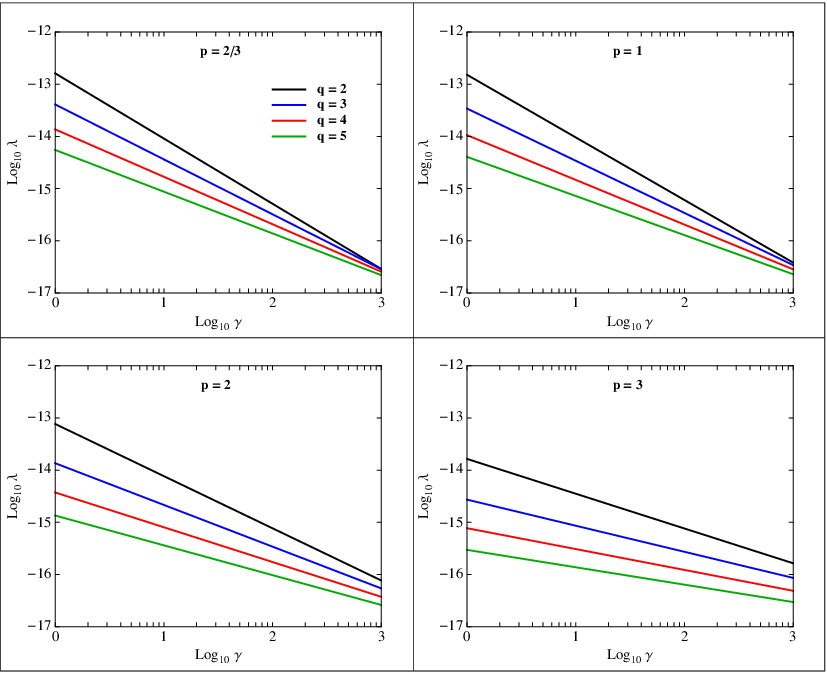
where we have set . Figure 2 shows the value of the parameter as a function of the dissipation strength , obtained from the expression in Eq. (75), setting the value of the power spectrum equal to the observed value by PLANCK in Eq. (19) and the value of given in Eq. (26). In Fig. 2, we used the values (black), (blue), (red), and (green). The uncertainty associated with each yellow band depends on the uncertainties on and , given by
| (76) |
The first term in Eq. (76) is much smaller than the second one, so that most of the uncertainty on comes from the measurement of .
Taking for example , we estimate the order of magnitude of some important quantities in the theory, as reported in Table 1. The mass of the the inflaton field has been obtained assuming a quadratic potential , or .
| Coupling | |
|---|---|
| Tensor-to-scalar ratio | |
| Inflaton mass | |
| Potential height | |
| Hubble rate | |
| Dissipation parameter | |
| Radiation temperature | |
| Field excursion |
The expression for the tensor-to-scalar ratio in Eq. (71) can also be given in terms of by replacing with the value in Eq. (73), to obtain
| (77) |
In Fig. 3, we show the tensor-to-scalar ratio as a function of the dissipation strength , obtained from Eq. (77). For any value of , the values of the tensor-to-scalar ratio are much smaller than the bound in Eq. (37), set by the PLANCK mission. In particular, for we obtain a tensor-to-scalar ratio of the order of .

As discussed in Sec. 4.1, in cold inflation such a low value of is typical of small-field inflationary models [74].
We investigate the nature of monomial warm inflation by deriving the relation between the number of e-folds and the field excursion
For this, we first use the Friedmann equation to obtain the derivative of with respect to the inflaton field ,
| (78) |
The expression for the first slow-roll parameter is then
| (79) |
which can be expressed in terms of the number of e-folds in Eq. (59) and the expression for in Eq. (51) as
| (80) |
In the limit we obtain the result in the cold theory of inflation, while the strong-dissipation limit , which is the one relevant in this discussion, gives
| (81) |
Combining this latter equality with the consistency relation in Eq. (66), we finally obtain the expression for the field excursion in terms of the number of e-folds,
| (82) |
The number of e-folds required to inflate between the modes with CMB multipoles at horizon crossing is , while sufficient inflation requires as discussed earlier. This yields to a lower bound on the scalar field excursion as a function of , known in the literature as the “Lyth bound” [81]. In cold inflation models, the Lyth bound constrain large field theories to predict relatively large (observable) values of the tensor-to-scalar ratio. Here, Eq. (82) is thus the analogous formulation of the Lyth bound in warm inflation. We write as a fun‘ction of the dissipation strength only, by eliminating using Eq. (72) and the coupling using Eq. (74). Results are shown in Fig. 4 for the value of as a function of , with the potential of index , , , and .
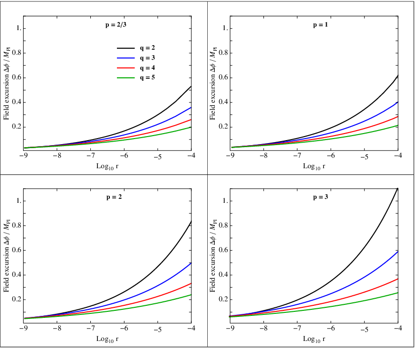
In warm inflation, the inflaton field might achieve a large excursion with negligible value of the tensor-to-scalar ratio , thus evading the prediction valid in cold inflation models. As evident from Eq. (82), this result is possible since is multiplied by the quantities and , which in the strong limit of warm inflation are both greater than one. The possibility that the ordinary Lyth bound might be evaded in warm inflation has been also discussed in Refs. [61, 32], and can be used to experimentally distinguish between warm and cold inflationary models, while the possibility of eluding the Lyth bound in cold inflation models with polynomial potentials has been considered in Ref. [82]. To sum up, warm inflation is one of the best motivated inflationary models to fit current observations. Monomial warm inflation naturally accommodates values of the tensor-to-scalar ratio which are much smaller than the current bound set by the BICEP2-PLANCK mission. For typical values of the parameters in the theory, we have obtained . At the same time, the inflaton field evolves spanning a large value , which in the cold theory of inflation is associated with a much larger tensor-to-scalar ratio than what obtained in monomial warm inflation. Using the observational value of the scalar spectral tilt , we have obtained a value of the coupling constant , which leads to an estimate of the parameters of the theory as in Table 1. The Hubble rate obtained is , which is safely within the bound given by Eq. (38) and is much smaller than thus justifying the strong dissipation treatment we adopted.
Acknowledgements.
The author would like to thank Øyvind Grøn (U. Oslo) for useful comments and for finding a mistake in an earlier version of this paper.References
- (1) D. Kazanas, Dynamics of the universe and spontaneous symmetry breaking, Astrophys. J. 241, L59 (1980).
- (2) A. A. Starobinsky, A new type of isotropic cosmological models without singularity, Phys. Lett. B 91, 99 (1980).
- (3) A. H. Guth, Inflationary universe: A possible solution to the horizon and flatness problems, Phys. Rev. D 23, 347 (1981).
- (4) K. Sato, Cosmological Baryon Number Domain Structure and the First Order Phase Transition of a Vacuum, Phys. Lett. B 99, 66 (1981).
- (5) V. F. Mukhanov and G. V. Chibisov, Quantum fluctuations and a nonsingular universe , JETP Lett. 33, 532 (1981).
- (6) A. Albrecht and P. J. Steinhardt, Cosmology for Grand Unified Theories with Radiatively Induced Symmetry Breaking, Phys. Rev. Lett. 48, 1220 (1982).
- (7) A. D. Linde, A new inflationary universe scenario: A possible solution of the horizon, flatness, homogeneity, isotropy and primordial monopole problems, Phys. Lett. B 108, 389 (1982).
- (8) A. D. Linde, Chaotic Inflation, Phys. Lett. B 129, 177 (1983).
- (9) V. F. Mukhanov, H. A. Feldman and R. H. Brandenberger, Theory of cosmological perturbations, Phys. Rept. 215, 203 (1992).
- (10) A. D. Linde, Particle Physics and Inflationary Cosmology, Harwood Academic, Switzerland (1990).
- (11) E. W. Kolb and M. S. Turner, The Early Universe, Addison-Wesley (1990).
- (12) L. Bergstrom and A. Goobar, Cosmology and Particle Astrophysics, Springer Praxis (2004).
- (13) S. Weinberg, Cosmology, Oxford University Press, USA (2008).
- (14) C. L. Bennett et al. (WMAP Collaboration), First Year Wilkinson Microwave Anisotropy Probe (WMAP) Observations: Preliminary Maps and Basic Results, Astrophys. J. Suppl. Ser. 148, 1 (2003) [astro-ph/0302207].
- (15) C. L. Bennett et al. (WMAP Collaboration), Nine-Year Wilkinson Microwave Anisotropy Probe (WMAP) Observations: Final Maps and Results, Astrophys. J. Suppl. 208, 20 (2013) [astro-ph/1212.5225].
- (16) A. H. Guth and S. Y. Pi, Fluctuations in the New Inflationary Universe, Phys. Rev. Lett. 49, 1110 (1982).
- (17) S. W. Hawking, The development of irregularities in a single bubble inflationary universe, Phys. Lett. B 115, 295 (1982).
- (18) A. A. Starobinsky, Dynamics of phase transition in the new inflationary universe scenario and generation of perturbations, Phys. Lett. B 117, 175 (1982).
- (19) J. M. Bardeen, P. J. Steinhardt and M. S. Turner, Spontaneous creation of almost scale-free density perturbations in an inflationary universe, Phys. Rev. D 28, 679 (1983).
- (20) P. J. Steinhardt and M. S. Turner, Prescription for successful new inflation, Phys. Rev. D 29, 2162 (1984).
- (21) A. Albrecht, P. J. Steinhardt, M. S. Turner and F. Wilczek, Reheating an Inflationary Universe, Phys. Rev. Lett. 48, 1437 (1982).
- (22) L. F. Abbott, E. Farhi and M. B. Wise, Particle production in the new inflationary cosmology, Phys. Lett. B 117, 29 (1982).
- (23) M. Morikawa and M. Sasaki, Entropy Production In The Inflationary Universe, Prog. Theor. Phys. 72, 782 (1984).
- (24) A. Hosoya and M.-aki Sakagami, Time development of Higgs field at finite temperature, Phys. Rev. D 29, 2228 (1984).
- (25) I. G. Moss, Primordial inflation with spontaneous symmetry breaking, Phys. Lett. B 154, 120 (1985).
- (26) S. R. Lonsdale and I. G. Moss, A superstring cosmological model, Phys. Lett. B 189, 12 (1987).
- (27) J. Yokoyama and K. Maeda, On the Dynamics of the Power Law Inflation Due to an Exponential Potential, Phys. Lett. B 207, 31 (1988).
- (28) A. R. Liddle, Power Law Inflation With Exponential Potentials, Phys. Lett. B 220, 502 (1989).
- (29) A. Berera and L. Z. Fang, Thermally Induced Density Perturbations in the Inflation Era, Phys. Rev. Lett. 74, 1912 (1995) [astro-ph/9501024].
- (30) A. Berera, Warm Inflation, Phys. Rev. Lett. 75, 3218 (1995) [astro-ph/9509049].
- (31) A. Berera, I. G. Moss and R. O. Ramos, Warm Inflation and its Microphysical Basis, Rept. Prog. Phys. 72, 026901 (2009) [hep-ph/0808.1855].
- (32) S. Bartrum, M. Bastero-Gil, A. Berera, R. Cerezo, R. O. Ramos, and J. G. Rosa, The importance of being warm (during inflation), Phys. Lett. B 732, 116 (2014) [hep-ph/1307.5868].
- (33) R. O. Ramos and L. A. da Silva, Power spectrum for inflation models with quantum and thermal noises, JCAP 1303, 032 (2013) [astro-ph/1302.3544].
- (34) M. Bastero-Gil, A. Berera and R. O. Ramos, Dissipation coefficients from scalar and fermion quantum field interactions, JCAP 1109, 033 (2011) [hep-ph/1008.1929].
- (35) M. Bastero-Gil, A. Berera, R. O. Ramos, and J. G. Rosa, General dissipation coefficient in low-temperature warm inflation, JCAP 1301, 016 (2013) [hep-ph/1207.0445].
- (36) M. Bastero-Gil, A. Berera, R. O. Ramos, and J. G. Rosa, Observational implications of mattergenesis during inflation, JCAP 1410, 053 (2014) [astro-ph/1404.4976].
- (37) A. Berera, Warm Inflation in the Adiabatic Regime- a Model, an Existence Proof for Inflationary Dynamics in Quantum Field Theory, Nucl. Phys. B 595, 666 (2000) [hep-ph/9904409].
- (38) A. N. Taylor and A. Berera, Perturbation spectra in the warm inflationary scenario, Phys. Rev. D 62, 083517 (2000) [astro-ph/0006077].
- (39) L. M. H. Hall, I. G. Moss, A. Berera, Scalar perturbation spectra from warm inflation, Phys. Rev. D 69 083525 (2004) [astro-ph/0305015].
- (40) M. Gleiser and R. O. Ramos, Microphysical Approach to Nonequilibrium Dynamics of Quantum Fields, Phys. Rev. D 50, 2441 (1994) [hep-ph/9311278].
- (41) A. Berera, M. Gleiser and R. O. Ramos, Strong dissipative behavior in quantum field theory, Phys. Rev. D 58, 123508 (1998) [hep-ph/9803394].
- (42) J. Yokoyama and A. D. Linde, Is Warm Inflation Possible?, Phys. Rev. D 60, 083509 (1999) [hep-ph/9809409].
- (43) I. G. Moss and C. Xiong, Non-gaussianity in fluctuations from warm inflation, JCAP 0704, 007 (2007) [astro-ph/0701302].
- (44) I. G. Moss and T. Yeomans, Non-gaussianity in the strong regime of warm inflation, JCAP 1108, 009 (2011) [astro-ph/1102.2833].
- (45) A. Berera and R. O. Ramos, Dynamics of Interacting Scalar Fields in Expanding Space-Time, Phys. Rev. D 71, 023513 (2005) [hep-ph/0406339].
- (46) S. del Campo, R. Herrera and D. Pavon, Cosmological perturbations in warm inflationary models with viscous pressure, Phys. Rev. D 75, 083518 (2007) [astro-ph/0703604].
- (47) I. G. Moss and C. Xiong, On the consistency of warm inflation, JCAP 0811, 023 (2008) [astro-ph/0808.0261].
- (48) C. Graham and I. G. Moss, Density fluctuations from warm inflation, JCAP 0907, 013 (2009) [astro-ph/0905.3500].
- (49) L. Visinelli, Cosmological perturbations for an inflaton field coupled to radiation, JCAP 1501, 005 (2015) [astro-ph/1410.1187].
- (50) A. Berera and R. O. Ramos, Construction of a robust warm inflation mechanism, Phys. Lett. B 567, 294 (2003) [hep-ph/0210301].
- (51) M. Bastero-Gil and A. Berera, Sneutrino warm inflation in the minimal supersymmetric model, Phys. Rev. D 72,103526 (2005) [hep-ph/0507124].
- (52) M. Bastero-Gil and A. Berera, Determining the regimes of cold and warm inflation in the supersymmetric hybrid model, Phys. Rev. D 71, 063515 (2005) [hep-ph/0411144].
- (53) I. G. Moss and C. Xiong, Dissipation coefficients for supersymmetric inflatonary models, [hep-ph/0603266] (2006).
- (54) T. Matsuda, Aspects of warm-flat directions, Int. J. Mod. Phys. A 25, 4221 (2010) [hep-th/0908.3059].
- (55) M. Bastero-Gil, A. Berera, R. O. Ramos and J. G. Rosa, Warm Little Inflaton, [hep-ph/1604.08838] (2016).
- (56) P. A. R. Ade et al. [Planck Collaboration], Planck 2013 results. XVI. Cosmological parameters, Astron. Astrophys. 571, A16 (2014) [astro-ph/1303.5076].
- (57) H. P. De Oliveira and S. E. Jorás, On Perturbations in Warm Inflation, Phys. Rev. D 64, 063513 (2001) [gr-qc/0103089].
- (58) H. P. De Oliveira, Density perturbations in warm inflation and COBE normalization, Phys. Lett. B 526, 1 (2002) [gr-qc/0202045].
- (59) G. Smoot et al, Structure in the COBE differential microwave radiometer first-year maps, Astrophys. J. 396, L1 (1992).
- (60) L. Visinelli, Natural Warm Inflation, JCAP 1109, 013 (2011) [astro-ph/1107.3523].
- (61) Y.-F. Cai, J. B. Dent and D. A. Easson, Warm DBI Inflation, Phys. Rev. D 83, 101301 (2011) [hep-th/1011.4074].
- (62) A. R. Liddle, P. Parsons and J. D. Barrow, Formalizing the slow-roll approximation in inflation, Phys. Rev. D 50, 7222 (1994) [astro-ph/9408015].
- (63) A. Kosowsky, M S. Turner, CBR Anisotropy and the Running of the Scalar Spectral Index, Phys. Rev. D 52, 1739 (1995) [astro-ph/9504071].
- (64) S. M. Leach and A. R. Liddle, Microwave background constraints on inflationary parameters, Mon. Not. Roy. Astron. Soc. 341, 1151 (2003) [astro-ph//0207213].
- (65) A. R. Liddle and S. M. Leach, How long before the end of inflation were observable perturbations produced?, Phys. Rev. D 68, 103503 (2003) [astro-ph/0305263].
- (66) J. Schwinger, Brownian motion of a quantum oscillator, J. Math. Phys. 2, 407 (1961).
- (67) L. V. Keldysh, Diagram Technique for Non-equilibrium Processes, J. Exptl. Theoret. Phys. 47, 1515 (1964) [http://www.jetp.ac.ru].
- (68) J. Rammer and H. Smith, Quantum field-theoretical methods in transport theory of metals, Rev. Mod. Phys. 58, 323 (1986).
- (69) E. Calzetta and B. L. Hu, Stochastic dynamics of correlations in quantum field theory: From Schwinger-Dyson to Boltzmann-Langevin equation, Phys. Rev. D 61, 025012 (2000) [hep-ph/9903.291].
- (70) P. A. R. Ade et al. [BICEP2 and Keck Array Collaborations], BICEP2 / Keck Array V: Measurements of B-mode Polarization at Degree Angular Scales and 150 GHz by the Keck Array, Astrophys. J. 811,126 (2015) [astro-ph/1502.00643].
- (71) P. A. R. Ade et al. [BICEP2 and Planck Collaborations], A Joint Analysis of BICEP2/Keck Array and Planck Data, Phys. Rev. Lett. 114, 101301 (2015) [astro-ph/1502.00612].
- (72) D. H. Lyth, A bound on inflationary energy density from the isotropy of the microwave background, Phys. Lett. B 147, 403L (1984).
- (73) F. C. Adams, K. Freese and A. H. Guth, Constraints on the scalar-field potential in inflationary models, Phys. Rev. D 43, 965 (1991).
- (74) D. H. Lyth, Particle physics models of inflation, Lect. Notes Phys. 738, 81 (2008).
- (75) T. Piran and R. M. Williams, Inflation in universes with a massive scalar field, Phys. Lett. B 163, 331 (1985).
- (76) V. A. Belinsky, I. M. Khalatnikov, L. P. Grishchuk and Y. B. Zeldovich, Inflationary Stages In Cosmological Models With A Scalar Field, Phys. Lett. B 155, 232 (1985).
- (77) P. Creminelli, D. L. Nacir, M. Simonovi, G. Trevisan and M. Zaldarriaga, or Not : Testing the Simplest Inflationary Potential, Phys. Rev. Lett. 112, 241303 (2014) [astro-ph/1404.1065].
- (78) D. H. Lyth, Inflation with TeV-scale gravity, Phys. Lett. B 448, 191 (1999) [hep-ph/9810320].
- (79) E. Silverstein and A. Westphal, Monodromy in the CMB: Gravity Waves and String Inflation, Phys. Rev. D 78, 106003 (2008) [hep-th/0803.3085].
- (80) L. McAllister, E. Silverstein and A. Westphal, Gravity Waves and Linear Inflation from Axion Monodromy, Phys. Rev. D 82, 046003 (2010) [hep-th/0808.0706].
- (81) D. H. Lyth, What would we learn by detecting a gravitational wave signal in the cosmic microwave background anisotropy?, Phys. Rev. Lett. 78, 1861 (1997) [hep-th/9606387].
- (82) S. Hotchkiss, A. Mazumdar and S. Nadathur, Observable gravitational waves from inflation with small field excursions, JCAP 1202, 008 (2012) [astro-ph/1110.5389].