Piece-wise quadratic approximations of arbitrary error functions for fast and robust machine learning
Abstract
Most of machine learning approaches have stemmed from the application of minimizing the mean squared distance principle, based on the computationally efficient quadratic optimization methods. However, when faced with high-dimensional and noisy data, the quadratic error functionals demonstrated many weaknesses including high sensitivity to contaminating factors and dimensionality curse. Therefore, a lot of recent applications in machine learning exploited properties of non-quadratic error functionals based on norm or even sub-linear potentials corresponding to quasinorms (). The back side of these approaches is increase in computational cost for optimization. Till so far, no approaches have been suggested to deal with arbitrary error functionals, in a flexible and computationally efficient framework. In this paper, we develop a theory and basic universal data approximation algorithms (-means, principal components, principal manifolds and graphs, regularized and sparse regression), based on piece-wise quadratic error potentials of subquadratic growth (PQSQ potentials). We develop a new and universal framework to minimize arbitrary sub-quadratic error potentials using an algorithm with guaranteed fast convergence to the local or global error minimum. The theory of PQSQ potentials is based on the notion of the cone of minorant functions, and represents a natural approximation formalism based on the application of min-plus algebra. The approach can be applied in most of existing machine learning methods, including methods of data approximation and regularized and sparse regression, leading to the improvement in the computational cost/accuracy trade-off. We demonstrate that on synthetic and real-life datasets PQSQ-based machine learning methods achieve orders of magnitude faster computational performance than the corresponding state-of-the-art methods, having similar or better approximation accuracy.
Keywords:
data approximation , nonquadratic potential , principal components , clustering , regularized regression , sparse regression1 Introduction
Modern machine learning and artificial intelligence methods are revolutionizing many fields of science today, such as medicine, biology, engineering, high-energy physics and sociology, where large amounts of data have been collected due to the emergence of new high-throughput computerized technologies. Historically and methodologically speaking, many machine learning algorithms have been based on minimizing the mean squared error potential, which can be explained by tractable properties of normal distribution and existence of computationally efficient methods for quadratic optimization. However, most of the real-life datasets are characterized by strong noise, long-tailed distributions, presence of contaminating factors, large dimensions. Using quadratic potentials can be drastically compromised by all these circumstances: therefore, a lot of practical and theoretical efforts have been made in order to exploit the properties of non-quadratic error potentials which can be more appropriate in certain contexts. For example, methods of regularized and sparse regression such as lasso and elastic net based on the properties of metrics [1, 2] found numerous applications in bioinformatics [3], and norm-based methods of dimension reduction are of great use in automated image analysis [4]. Not surprisingly, these approaches come with drastically increased computational cost, for example, connected with applying linear programming optimization techniques which are substantially more expensive compared to mean squared error-based methods.
In practical applications of machine learning, it would be very attractive to be able to deal with arbitrary error potentials, including those based on or fractional quasinorms (), in a computationally efficient and scalable way. There is a need in developing methods allowing to tune the computational cost/accuracy of optimization trade-off accordingly to various contexts.
In this paper, we suggest such a universal framework able to deal with a large family of error potentials. We exploit the fact that finding a minimum of a piece-wise quadratic function, or, in other words, a function which is the minorant of a set of quadratic functionals, can be almost as computationally efficient as optimizing the standard quadratic potential. Therefore, if a given arbitrary potential (such as -based or fractional quasinorm-based) can be approximated by a piece-wise quadratic function, this should lead to relatively efficient and simple optimization algorithms. It appears that only potentials of quadratic or subquadratic growth are possible in this approach: however, these are the most usefull ones in data analysis. We introduce a rich family of piece-wise quadratic potentials of subquadratic growth (PQSQ-potentials), suggest general approach for their optimization and prove convergence of a simple iterative algorithm in the most general case. We focus on the most used methods of data dimension reduction and regularized regression: however, potential applications of the approach can be much wider.
Data dimension reduction by constructing explicit low-dimensional approximators of a finite set of vectors is one of the most fundamental approach in data analysis. Starting from the classical data approximators such as -means [5] and linear principal components (PCA) [6], multiple generalizations have been suggested in the last decades (self-organizing maps, principal curves, principal manifolds, principal graphs, principal trees, etc.)[7, 8] in order to make the data approximators more flexible and suitable for complex data structures.
We solve the problem of approximating a finite set of vectors (data set) by a simpler object embedded into the data space, such that for each point an approximation error function can be defined. We assume this function in the form
| (1) |
where the upper stands for the coordinate index, and is a monotonously growing symmetrical function, which we will be calling the error potential. By data approximation we mean that the embedment of in the data space minimizes the error
Note that our definition of error function is coordinate-wise (it is a sum of error potential over all coordinates).
The simplest form of the error potential is quadratic , which leads to the most known data approximators: mean point ( is a point), principal points ( is a set of points) [9], principal components ( is a line or a hyperplane) [6]. In more advanced cases, can posses some regular properties leading to principal curves ( is a smooth line or spline) [10], principal manifolds ( is a smooth low-dimensional surface) and principal graphs (eg., is a pluri-harmonic graph embedment) [11, 7].
There exist multiple advantages of using quadratic potential , because it leads to the most computationally efficient algorithms usually based on the splitting schema, a variant of expectation-minimization approach [7]. For example, -means algorithm solves the problem of finding the set of principal points and the standard iterative Singular Value Decomposition finds principal components. However, quadratic potential is known to be sensitive to outliers in the data set. Also, purely quadratic potentials can suffer from the curse of dimensionality, not being able to robustly discriminate ‘close’ and ‘distant’ point neighbours in a high-dimensional space [12].
There exist several widely used ideas for increasing approximator’s robustness in presence of strong noise in data such as: (1) using medians instead of mean values, (2) substituting quadratic norm by norm (e.g. [13, 14]), (3) outliers exclusion or fixed weighting or iterative reweighting during optimizing the data approximators (e.g. [15, 16, 17]), and (4) regularizing the PCA vectors by norm [18, 19, 20]. In some works, it was suggested to utilize ‘trimming’ averages, e.g. in the context of the -means clustering or some generalizations of PCA [21, 14]). In the context of regression, iterative reweighting is exploited to mimic the properties of norm [22]. Several algorithms for constructing PCA with norm have been suggested [23, 24, 25] and systematically benchmarked [26, 27]. Some authors go even beyond linear metrics and suggests that fractional quasinorms () can be more appropriate in high-dimensional data approximation [12].
However, most of the suggested approaches exploiting properties of non-quadratic metrics either represent useful but still arbitrary heuristics or are not sufficiently scalable. The standard approach for minimizing -based norm consists in solving a linear programming task. Despite existence of many efficient linear programming optimizer implementations, by their nature these computations are much slower than the iterative methods used in the standard SVD algorithm or -means.
In this paper, we provide implementations of the standard data approximators (mean point, -means, principal components) using a PQSQ potential. As an other application of PQSQ-based framework in machine learning, we develop PQSQ-based regularized and sparse regression (imitating the properties of lasso and elastic net).
2 Piecewise quadratic potential of subquadratic growth (PQSQ)
2.1 Definition of the PQSQ potential
Let us split all non-negative numbers into non-intersecting intervals , for a set of thresholds . For convenience, let us denote . Piecewise quadratic potential is a continuous monotonously growing function constructed from pieces of centered at zero parabolas , defined on intervals , satisfying (see Figure 1):
| (2) |
| (3) |
| (4) |
where is a majorating function, which is to be approximated (imitated) by . For example, in the simplest case can be a linear function: , in this case, will approximate the -based error function.
Note that accordingly to (3,4), . Therefore, the choice of can naturally create a ‘trimmed’ version of error potential such that some data points (outliers) do not have any contribution to the gradient of , hence, will not affect the optimization procedure. However, this set of points can change during minimizaton of the potential.
The condition of subquadratic growth consists in the requirement and . To guarantee this, the following simple condition on should be satisfied:
| (5) |
Therefore, is a monotonic concave function of :
In particular, should grow not faster than any parabola , which is tangent to .

2.2 Basic approach for optimization
In order to use the PQSQ potential in an algorithm, a set of interval thresholds for each coordinate should be provided. Matrices of and coefficients defined by (3,4) based on interval definitions: , , are computed separately for each coordinate .
Minimization of PQSQ-based functional consists in several basic steps which can be combined in an algorithm:
1) For each coordinate , split all data point indices into non-overlapping sets :
| (6) |
where is a matrix which depends on the nature of the algorithm.
2) Minimize PQSQ-based functional where each set of points contributes to the functional quadratically with coefficient . This is a quadratic optimization task.
3) Repeat (1)-(2) till convergence.
3 General theory of the piece-wise convex potentials as the cone of minorant functions
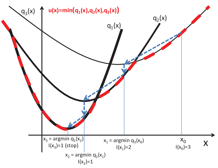
In order to deal in most general terms with the data approximation algorithms based on PQSQ potentials, let us consider a general case where a potential can be constructed from a set of functions with only two requirements: 1) that each has a (local) minimum; 2) that the whole set of all possible s forms a cone. In this case, instead of the operational definition (2) it is convenient to define the potential as the minorant function for a set of functions as follows. For convenience, in this section, will notify a vector .
Let us consider a generating cone of functions . We remind that the definition of a cone implies that for any , we have , where .
It is convinient to introduce a multiindex
indicating which particular function(s) corresponds to the value of , i.e.
| (8) |
For a cone let us define a set of all possible minorant functions
| (9) |
Proposition 1
is a cone.
For any two minorant functions
we have
| (10) |
where is a set of all possible linear combinations of functions from and .
Proposition 2
Any restriction of onto a linear manifold is a cone.
Let us denote a restriction of function onto , i.e. . is a part of . Set of all forms a restriction of onto . is a cone, hence, is a cone (Proposition 1).
Theorem 3.1
Splitting algorithm (Algorithm 1) for minimizing converges in a finite number of steps.
Since the set of functions is finite then we only have to show that at each step the value of the function can not increase. For any and the value for we can have only two cases:
(1) Either (convergence, and in this case for any );
Note that in Algorithm 1 we do not specify exactly the way to find the local minimum of . To be practical, the cone should contain only functions for which finding a local minimum is fast and explicit. Evident candidates for this role are positively defined quadratic functionals , where is a positively defined symmetric matrix. Any minorant function (7) constructed from positively defined quadratic functions will automatically provide subquadratic growth, since the minorant can not grow faster than any of the quadratic forms by which it is defined.
Operational definition of PQSQ given above (2), corresponds to a particular form of the quadratic functional, with being diagonal matrix. This choice corresponds to the coordinate-wise definition of data approximation error function (1) which is particularly simple to minimize. This circumstance is used in Algorithms 2,3.
4 Commonly used data approximators with PQSQ potential
4.1 Mean value and -means clustering in PQSQ approximation measure
Mean vector for a set of vectors , and an approximation error defined by potential can be defined as a point minimizing the mean error potential for all points in :
| (11) |
For Euclidean metrics () it is the usual arithmetric mean.
For metrics (), (11) leads to the implicit equation , where stands for the number of points, which corresponds to the definition of median. This equation can have a non-unique solution in case of even number of points or when some data point coordinates coincide: therefore, definition of median is usually accompanied by heuristics used for breaking ties, i.e. to deal with non-uniquely defined rankings. This situation reflects the general situation of existence of multiple local minimuma and possible non-uniqueness of global minimum of (11) (Figure 3).
For PQSQ approximation measure (2) it is difficult to write down an explicit formula for computing the mean value corresponding to the global minimum of (11). In order to find a point minimizing mean potential, a simple iterative algorithm can be used (Algorithm 2). The suggested algorithm converges to the local minimum which depends on the initial point approximation.
Based on the PQSQ approximation measure and the algorithm for computing the PQSQ mean value (Algorithm 2), one can construct the PQSQ-based -means clustering procedure in the usual way, splitting estimation of cluster centroids given partitioning of the data points into disjoint groups, and then re-calculating the partitioning using the PQSQ-based proximity measure.

4.2 Principal Component Analysis (PCA) in PQSQ metrics
Accordingly to the classical definition of the first principal component, it is a line best fit to the data set [6]. Let us define a line in the parametric form , where is the parameter. Then the first principal component will be defined by vectors satisfying
| (12) |
where
| (13) |
The standard first principal component (PC1) corresponds to when the vectors can be found by a simple iterative splitting algorithm for Singular Value Decomposition (SVD). If does not contain missing values then is the vector of arithmetic mean values. By contrast, computing -based principal components () represents a much more challenging optimization problem [25]. Several approximative algorithms for computing -norm PCA have been recently suggested and benchmarked [23, 24, 25, 26, 27]. To our knowledge, there have not been a general efficient algorithm suggested for computing PCA in case of arbitrary approximation measure for some monotonous function .
Computing PCA based on PQSQ approximation error is only slightly more complicated than computing the standard PCA by SVD. Here we provide a pseudo-code (Algorithm 3) of a simple iterative algorithm (similar to Algorithm 2) with guaranteed convergence (see Section 3).
Computation of second and further principal components follows the standard deflation approach: projections of data points onto the previously computed component are subtracted from the data set, and the algorithm is applied to the residues. However, as it is the case in any non-quadratic metrics, the resulting components can be non-orthogonal or even not invariant with respect to the dataset rotation. Moreover, unlike -based principal components, the Algorithm 3 does not always converge to a unique global minimum; the computed components can depend on the initial estimate of . The situation is somewhat similar to the standard -means algorithm. Therefore, in order to achieve the least possible approximation error to the linear subspace, can be initialized randomly or by data vectors many times and the deepest in PQSQ approximation error (1) minimum should be selected.
How does the Algorithm 1 serve a more abstract version of the Algorithms 2,3? For example, the ‘variance’ function to be minimized in Algorithm 2 uses the generating functions in the form , where is the index of the interval in (2). Hence, is a minorant function, belonging to the cone , and must converge (to a local minimum) in a finite number of steps accordingly to Theorem 3.1.
4.3 Nonlinear methods: PQSQ-based Principal
Graphs and Manifolds
In a series of works, the authors of this article introduced a family of methods for constructing principal objects based on graph approximations (e.g., principal curves, principal manifolds, principal trees), which allows constructing explicit non-linear data approximators (and, more generally, approximators with non-trivial topologies, suitable for approximating, e.g., datasets with branching or circular topology) [28, 29, 30, 31, 11, 8, 7, 32]. The methodology is based on optimizing a piece-wise quadratic elastic energy functional (see short description below). A convenient graphical user interface was developed with implementation of some of these methods [33].
Let be a simple undirected graph with set of vertices and set of edges . For a -star in is a subgraph with vertices and edges . Suppose for each , a family of -stars in has been selected. We call a graph with selected families of -stars an elastic graph if, for all and , the correspondent elasticity moduli and are defined. Let be vertices of an edge and be vertices of a -star (among them, is the central vertex).
For any map the energy of the graph is defined as
For a given map we divide the dataset into node neighborhoods . The set contains the data points for which the node is the closest one in . The energy of approximation is:
| (14) |
where are the point weights. Simple and fast algorithm for minimization of the energy
| (15) |
is the splitting algorithm, in the spirit of the classical -means clustering: for a given system of sets we minimize (optimization step, it is the minimization of a positive quadratic functional), then for a given we find new (re-partitioning), and so on; stop when no change.
Application of PQSQ-based potential is straightforward in this approach. It consists in replacing (14) with
where is a chosen PQSQ-based error potential. Partitioning of the dataset into can be also based on calculating the minimum PQSQ-based error to , or can continue enjoying nice properties of -based distance calculation.
5 PQSQ-based regularized regression
5.1 Regularizing linear regression with PQSQ potential
One of the major application of non-Euclidean norm properties in machine learning is using non-quadratic terms for penalizing large absolute values of regression coefficients [1, 2]. Depending on the chosen penalization term, it is possible to achieve various effects such as sparsity or grouping coefficients for redundant variables. In a general form, regularized regression solves the following optimization problem
| (16) |
where is the number of observations, is the number of independent variables in the matrix , are dependent variables (to be predicted), is an internal parameter controlling the strength of regularization (penalty on the amplitude of regression coefficients ), and is the regularizer function, which is for ridge regression, for lasso and for elastic net methods correspondingly.
Here we suggest to imitate with a potential function, i.e. instead of (16) solving the problem
| (17) |
where is a PQSQ potential imitating arbitrary subquadratic regression regularization penalty.
Solving (17) is equivalent to iteratively solving a system of linear equations
| (18) |
where constant (where index is defined from ) is computed accordingly to the definition of function (see (3)), given the estimation of regression coefficients at the current iteration. In practice, iterating (18) converges in a few iterations, therefore, the algorithm can work very fast and outperform the widely used least angle regression algorithm for solving (16) in case of penalties.
5.2 Introducing sparsity by ‘black hole’ trick
Any PQSQ potential is characterized by zero derivative for by construction: , which means that the solution of (17) does not have to be sparse for any . Unlike pure -based penalty, the coefficients of regression diminish with increase of but there is nothing to shrink them to exact zero values, similar to the ridge regression. However, it is relatively straightforward to modify the algorithm, to achieve sparsity of the regression solution. The ’black hole’ trick consists in eliminating from regression training after each iteration (18) all regression coefficients smaller by absolute value than a given parameter (’black hole radius’). Those regression coefficients which have passed the ’black hole radius’ are put to zero and do not have any chance to change their values in the next iterations.

The optimal choice of value requires a separate study. From general considerations, it is preferable that the derivative would not be very close to zero. As a pragmatic choice for the numerical examples in this article, we define as the midst of the smallest interval in the definition of PQSQ potential (see Figure 4), i.e. , which guarantees far from zero . It might happen that this value of would collapse all to zero even without regularization (i.e., with ). In this case, the ’black hole radius’ is divided by half and it is checked that for the iterations would leave at list half of the regression coefficients. If it is not the case then the process of diminishing the ’black hole radius’ repeated recursively till meeting the criterion of preserving the majority of regression coefficients. In practice, it requires only few (very fast) additional iterations of the algorithm.
As in the lasso methodology, the problem (17) is solved for a range of values, calibrated such that the minimal would select the maximum number of regression variables, while the maximum value would lead to the most sparse regression (selecting only one single non-zero regression coefficient).
6 Numerical examples
6.1 Practical choices of parameters
The main parameters of PQSQ are (a) majorating function and (b) decomposition of each coordinate range into non-overlapping intervals. Depending on these parameters, various approximation error properties can be exploited, including those providing robustness to outlier data points.
When defining the intervals , it is desirable to achieve a small difference between and for expected argument values (differences between an estimator and the data point), and choose the suitable value of the potential trimming threshold in order to achieve the desired robustness properties. If no trimming is needed, then should be made larger than the maximum expected difference between coordinate values (maximum ).
In our numerical experiments we used the following definition of intervals. For any data coordinate , we define a characteristic difference , for example
| (19) |
where is a scaling parameter, which can be put at 1 (in this case, the approximating potential will not be trimmed). In case of existence of outliers, for defining , instead of amplitude one can use other measures such as the median absolute deviation (MAD):
| (20) |
in this case, the scaling parameter should be made larger, i.e. , if no trimming is needed.
After defining we use the following definition of intervals:
| (21) |
More sophisticated approaches are also possible to apply such as, given the number of intervals and the majorating function , choose in order to minimize the maximal difference
The calculation of intervals is straightforward for a given value of and many smooth concave functions like () or .
6.2 Implementation
We provide Matlab implementation of PQSQ approximators (in particular, PCA) together with the Matlab and R code used to generate the example figures in this article at ‘PQSQ-DataApproximators’ GitHub repository11 1 https://github.com/auranic/PQSQ-DataApproximators and Matlab implementation of PQSQ-based regularized regression with build-in imitations of (lasso-like) and mixture (elastic net-like) penalties at ‘PQSQ-regularized-regression’ GitHub repository22 2 https://github.com/Mirkes/PQSQ-regularized-regression/. The Java code implementing elastic graph-based non-linear approximator implementations is available from the authors on request.
6.3 Motivating example: dense two-cluster distribution contaminated by sparse noise
We demonstrate the value of PQSQ-based computation of -based PCA by constructing a simple example of data distribution consisting of a dense two-cluster component superimposed with a sparse contaminating component with relatively large variance whose co-variance does not coincide with the dense signal (Figure 5). We study the ability of PCA to withstand certain level of sparse contamination and compare it with the standard -based PCA. In this example, without noise the first principal component coincides with the vector connecting the two cluster centers: hence, it perfectly separates them in the projected distribution. Noise interferes with the ability of the first principal component to separate the clusters to the degree when the first principal component starts to match the principal variance direction of the contaminating distribution (Figure 5A,B). In higher dimensions, not only the first but also the first two principal components are not able to distinguish two clusters, which can hide an important data structure when applying the standard data visualization tools.
In the first test we study a switch of the first principal component from following the variance of the dense informative distribution (abscissa) to the sparse noise distribution (ordinate) as a function of the number of contaminating points, in (Figure 5A-C). We modeled two clusters as two 100-point samples from normal distribution centered in points and with isotropic variance with the standard deviation 0.1. The sparse noise distribution was modeled as a -point sample from the product of two Laplace distributions of zero means with the standard deviations 2 along abscissa and 4 along ordinate. The intervals for computing the PQSQ functional were defined by thresholds for each coordinate. Increasing the number of points in the contaminating distribution diminishes the average value of the abscissa coordinate of PC1, because the PC1 starts to be attracted by the contaminating distribution (Figure 5C). However, it is clear that on average PQSQ -based PCA is able to withstand much larger amplitude of the contaminating signal (very robust up to 20-30 points, i.e. 10-20% of strong noise contamination) compared to the standard -based PCA (which is robust to 2-3% of contamination).
In the second test we study the ability of the first two principal components to separate two clusters, in (Figure 5D-F). As in the first test, we modeled two clusters as two 100-point samples from normal distribution centered in points and with isotropic variance with the standard deviation 0.1 in all 100 dimensions. The sparse noise distribution is modeled as a -point sample from the product of 100 Laplace distributions of zero means with the standard deviations 1 along each coordinate besides the third coordinate (standard deviation of noise is 2) and the forth coordinate (standard deviation of noise is 4). Therefore, the first two principal component in the absence of noise are attracted by the dimensions 1 and 2, while in the presence of strong noise they are be attracted by dimensions 3 and 4, hiding the cluster structure of the dense part of the distribution. The definitions of the intervals were taken as in the first test. We measured the ability of the first two principal components to separate clusters by computing the -test between the two clusters projected in the 2D-space spanned by the first principal components of the global distribution (Figure 5D-F). As one can see, the average ability of the first principal components to separate clusters is significantly stronger in the case of PQSQ -based PCA which is able to separate robustly the clusters even in the presence of strong noise contamination (up to 80 noise points, i.e. 40% contamination).

6.4 Performance/stability trade-off benchmarking of -based PCA
In order to compare the computation time and the robustness of PQSQ-based PCA algorithm for the case with existing R-based implementations of -based PCA methods (pcaL1 package), we followed the benchmark described in [26]. We compared performance of PQSQ-based PCA based on Algorithm 3 with several -based PCA algorithms: L1-PCA* [25], L1-PCA [23], PCA-PP [34], PCA-L1 [24]. As a reference point, we used the standard PCA algorithm based on quadratic norm and computed using the standard SVD iterations.
The idea of benchmarking is to generate a series of datasets of the same size ( objects in dimensions) such that the first 5 dimensions would be sampled from a uniform distribution . Therefore, the first 5 dimensions represent ‘true manifold’ sampled by points.
The values in the last 5 dimensions represent ‘noise+outlier’ signal. The background noise is represented by Laplacian distribution of zero mean and 0.1 variance. The outlier signal is characterized by mean value , dimension and frequency . Then, for each data point with a probability , in the first outlier dimensions a value is drawn from . The rest of the values is drawn from background noise distribution.
As in [26], we’ve generated 1300 test sets corresponding to , with 100 examples for each combination of and .
For each test set 5 first principal components of unit length were computed, with corresponding point projection distributions and the mean vector . Therefore, for each initial data point , we have the ‘restored’ data point
For computing the PQSQ-based PCA we used 5 intervals without trimming. Changing the number of intervals did not significantly changed the benchmarking results.
Two characteristics were measured: (1) computation time measured as a ratio to the computation of 5 first principal components using the standard -based PCA and (2) the sum of absolute values of the restored point coordinates in the ‘outlier’ dimensions normalized on the number of points:

| (22) |
Formally speaking, is -based distance from the point projection onto the first five principal components to the ‘true’ subspace. In simplistic terms, larger values of correspond to the situation when the first five principal components do not represent well the first ‘true’ dimensions having significant loadings into the ‘outlier dimensions’. if and only if the first five components do not have any non-zero loadings in the dimensions .
The results of the comparison averaged over all 1300 test sets are shown in Figure 6. The PQSQ-based computation of PCA outperforms by accuracy the existing heuristics such as PCA-L1 but remains computationally efficient. It is 100 times faster than L1-PCA giving almost the same accuracy. It is almost 500 times faster than the L1-PCA* algorithm, which is, however, better in accuracy (due to being robust with respect to strong outliers). One can see from Figure 6 that PQSQ-based approach is the best in accuracy among fast iterative methods. The detailed tables of comparison for all combinations of parameters are available on GitHub33 3 http://goo.gl/sXBvqh. The scripts used to generate the datasets and compare the results can also be found there44 4 https://github.com/auranic/PQSQ-DataApproximators.
6.5 Comparing performances of PQSQ-based regularized regression and lasso algorithms
We compared performance of PQSQ-based regularized regression method imitating penalty with lasso implementation in Matlab, using 8 datasets from UCI Machine Learning Repository [35], Regression Task section. In the selection of datasets we chose very different numbers of objects and variables for regression construction (Table 1). All table rows containing missing values were eliminated for the tests.
| Dataset | Objects | Variables | lasso | PQSQ | Ratio |
|---|---|---|---|---|---|
| Breast cancer | 47 | 31 | 10.50 | 0.05 | 233.33 |
| Prostate cancer | 97 | 8 | 0.07 | 0.02 | 4.19 |
| ENB2012 | 768 | 8 | 0.53 | 0.03 | 19.63 |
| Parkinson | 5875 | 26 | 20.30 | 0.04 | 548.65 |
| Crime | 1994 | 100 | 10.50 | 0.19 | 56.24 |
| Crime reduced | 200 | 100 | 17.50 | 0.17 | 102.94 |
| Forest fires | 517 | 8 | 0.05 | 0.02 | 3.06 |
| Random regression (1000250) | 1000 | 250 | 2.82 | 0.58 | 4.86 |
We observed up to two orders of magnitude acceleration of PQSQ-based method compared to the lasso method implemented in Matlab (Table 1), with similar sparsity properties and approximation power as lasso (Figure 7).
While comparing time performances of two methods, we’ve noticed that lasso (as it is implemented in Matlab) showed worse results when the number of objects in the dataset approaches the number of predictive variables (see Table 1). In order to test this observation explicitly, we took a particular dataset (’Crime’) containing 1994 observations and 100 variables and compared the performance of lasso in the case of complete table and a reduced table (’Crime reduced’) containing only each 10th observation. Paradoxically, lasso converges almost two times slower in the case of the smaller dataset, while the PQSQ-based algorithm worked slightly faster in this case.
It is necessary to stress that here we compare the basic algorithms without many latest technical improvements which can be applied both to penalty and its PQSQ approximation (such as fitting the whole lasso path). Detailed comparison of all the existent modifications if far beyond the scope of this work.
For comparing approximation power of the PQSQ-based regularized regression and lasso, we used two versions of PQSQ potential for regression coefficients: with and without trimming. In order to represent the results, we used the ‘Number of non-zero parameters vs Fraction of Variance Unexplained (FVU)’ plots (see two representative examples at Figure 7). We suggest that this type of plot is more informative in practical applications than the ’lasso plot’ used to calibrate the strength of regularization, since it is a more explicit representation for optimizing the accuracy vs complexity ratio of the resulting regression.
From our testing, we can conclude that PQSQ-based regularized regression has similar properties of sparsity and approximation accuracy compared to lasso. It tends to slightly outperform lasso (to give smaller FVU) in case of . Introducing trimming in most cases does not change the best FVU for a given number of selected variables, but tends to decrease its variance (has a stabilization effect). In some cases, introducing trimming is the most advantageous method (Figure 7B).
The GitHub ‘PQSQ-regularized-regression’ repository contains exact dataset references and more complete report on comparing approximation ability of PQSQ-based regularized regression with lasso55 5 https://github.com/Mirkes/PQSQ-regularized-regression/wiki.

7 Conclusion
In this paper we develop a new machine learning framework (theory and application) allowing one to deal with arbitrary error potentials of not-faster than quadratic growth, imitated by piece-wise quadratic function of subquadratic growth (PQSQ error potential).
We develop methods for constructing the standard data approximators (mean value, -means clustering, principal components, principal graphs) for arbitrary non-quadratic approximation error with subquadratic growth and regularized linear regression with arbitrary subquadratic penalty by using a piecewise-quadratic error functional (PQSQ potential). These problems can be solved by applying quasi-quadratic optimization procedures, which are organized as solutions of sequences of linear problems by standard and computationally efficient algorithms.
| Data approximation/Clustering/Manifold learning | |
| Principal Component Analysis | Includes robust trimmed version of PCA, -based PCA, regularized PCA, and many other PCA modifications |
| Principal curves and manifolds | Provides possibility to use non-quadratic data approximation terms and trimmed robust version |
| Self-Organizing maps | Same as above |
| Principal graphs/trees | Same as above |
| K-means | Can include adaptive error potentials based on estimated error distributions inside clusters |
| High-dimensional data mining | |
| Use of fractional quasinorms () | Introducing fractional quasinorms in existing data-mining techniques can potentially deal with the curse of dimensionality, helping to better distinguish close from distant data points [12] |
| Regularized and sparse regression | |
| Lasso | Application of PQSQ-based potentials leads to speeding up in case of large and datasets |
| Elastic net | Same as above |
The suggested methodology have several advantages over existing ones:
(a) Scalability: the algorithms are computationally efficient and can be applied to large data sets containing millions of numerical values.
(b) Flexibility: the algorithms can be adapted to any type of data metrics with subquadratic growth, even if the metrics can not be expressed in explicit form. For example, the error potential can be chosen as adaptive metrics [36, 37].
(c) Built-in (trimmed) robustness: choice of intervals in PQSQ can be done in the way to achieve a trimmed version of the standard data approximators, when points distant from the approximator do not affect the error minimization during the current optimization step.
(d) Guaranteed convergence: the suggested algorithms converge to local or global minimum just as the corresponding predecessor algorithms based on quadratic optimization and expectation/minimization-based splitting approach.
In theoretical perspective, using PQSQ-potentials in data mining is similar to existing applications of min-plus (or, max-plus) algebras in non-linear optimization theory, where complex non-linear functions are approximated by infimum (or supremum) of finitely many ‘dictionary functions’ [38, 39]. We can claim that just as using polynomes is a natural framework for approximating in rings of functions, using min-plus algebra naturally leads to introduction of PQSQ-based functions and the cones of minorants of quadratic dictionary functions.
One of the application of the suggested methodology is approximating the popular in data mining metrics. We show by numerical simulations that PQSQ-based approximators perform as fast as the fast heuristical algorithms for computing -based PCA but achieve better accuracy in a previously suggested benchmark test. PQSQ-based approximators can be less accurate than the exact algorithms for optimizing -based functions utilizing linear programming: however, they are several orders of magnitude faster. PQSQ potential can be applied in the task of regression, replacing the classical Least Squares or -based Least Absolute Deviation methods. At the same time, PQSQ-based approximators can imitate a variety of subquadratic error potentials (not limited to or variations), including fractional quasinorms (). We demonstrate that the PQSQ potential can be easily adapted to the problems of sparse regularized regression with non-quadratic penalty on regression coefficients (including imitations of lasso and elastic net). On several real-life dataset examples we show that PQSQ-based regularized regression can perform two orders of magnitude faster than the lasso algorithm implemented in the same programming environment.
To conclude, in Table 2 we list possible applications of the PQSQ-based framework in machine learning.
Aknowledgement
This study was supported in part by Big Data Paris Science et Lettre Research University project ‘PSL Institute for Data Science’.
References
- [1] R. Tibshirani, Regression shrinkage and selection via the lasso, Journal of the Royal Statistical Society. Series B (Methodological) (1996) 267–288.
- [2] H. Zou, T. Hastie, Regularization and variable selection via the elastic net, Journal of the Royal Statistical Society: Series B (Statistical Methodology) 67 (2005) 301–320.
- [3] E. Barillot, L. Calzone, P. Hupe, J.-P. Vert, A. Zinovyev, Computational Systems Biology of Cancer, Chapman & Hall, CRC Mathemtical and Computational Biology, 2012.
- [4] J. Wright, Y. Ma, J. Mairal, G. Sapiro, T. S. Huang, S. Yan, Sparse representation for computer vision and pattern recognition, Proceedings of the IEEE 98 (2010) 1031–1044.
- [5] S. Lloyd, Last square quantization in pcm’s, Bell Telephone Laboratories Paper (1957).
- [6] K. Pearson, On lines and planes of closest fit to systems of points in space, Philos. Mag. 2 (1901) 559–572.
- [7] A. N. Gorban, A. Zinovyev, Principal graphs and manifolds, In Handbook of Research on Machine Learning Applications and Trends: Algorithms, Methods and Techniques, eds. Olivas E.S., Guererro J.D.M., Sober M.M., Benedito J.R.M., Lopes A.J.S. (2009).
- [8] A. Gorban, B. Kegl, D. Wunsch, A. Zinovyev (Eds.), Principal Manifolds for Data Visualisation and Dimension Reduction, LNCSE 58, Springer, 2008.
- [9] B. Flury, Principal points, Biometrika 77 (1990) 33–41.
- [10] T. Hastie, Principal curves and surfaces, PhD Thesis, Stanford University, California (1984).
- [11] A. N. Gorban, N. R. Sumner, A. Y. Zinovyev, Topological grammars for data approximation, Applied Mathematics Letters 20 (2007) 382–386.
- [12] C. C. Aggarwal, A. Hinneburg, D. A. Keim, On the surprising behavior of distance metrics in high dimensional space, in: Database Theory - ICDT 2001, 8th International Conference, London, UK, January 4-6, 2001, Proceedings, Springer, 2001, pp. 420–434.
- [13] C. Ding, D. Zhou, X. He, H. Zha, R1-PCA: rotational invariant L1-norm principal component analysis for robust subspace factorization, ICML (2006) 281–288.
- [14] S. Hauberg, A. Feragen, M. J. Black, Grassmann averages for scalable robust pca, in: Computer Vision and Pattern Recognition (CVPR), 2014 IEEE Conference on, IEEE, pp. 3810–3817.
- [15] L. Xu, A. L. Yuille, Robust principal component analysis by self-organizing rules based on statistical physics approach, Neural Networks, IEEE Transactions on 6 (1995) 131–143.
- [16] H. Allende, C. Rogel, S. Moreno, R. Salas, Robust neural gas for the analysis of data with outliers, in: Computer Science Society, 2004. SCCC 2004. 24th International Conference of the Chilean, IEEE, pp. 149–155.
- [17] T. Kohonen, Self-organizing Maps, Springer Series in Information Sciences, Vol.30, Berlin, Springer, 2001.
- [18] I. T. Jolliffe, N. T. Trendafilov, M. Uddin, A modified principal component technique based on the lasso, Journal of computational and Graphical Statistics 12 (2003) 531–547.
- [19] E. J. Candès, X. Li, Y. Ma, J. Wright, Robust principal component analysis?, Journal of the ACM (JACM) 58 (2011) 11.
- [20] H. Zou, T. Hastie, R. Tibshirani, Sparse principal component analysis, Journal of computational and graphical statistics 15 (2006) 265–286.
- [21] J. Cuesta-Albertos, A. Gordaliza, C. Matrán, et al., Trimmed -means: An attempt to robustify quantizers, The Annals of Statistics 25 (1997) 553–576.
- [22] C. Lu, Z. Lin, S. Yan, Smoothed low rank and sparse matrix recovery by iteratively reweighted least squares minimization., IEEE Trans Image Process 24 (2015) 646–654.
- [23] Q. Ke, T. Kanade, Robust l 1 norm factorization in the presence of outliers and missing data by alternative convex programming, in: Computer Vision and Pattern Recognition, 2005. CVPR 2005. IEEE Computer Society Conference on, volume 1, IEEE, pp. 739–746.
- [24] N. Kwak, Principal component analysis based on L1-norm maximization, Pattern Analysis and Machine Intelligence, IEEE Transactions on 30 (2008) 1672–1680.
- [25] J. Brooks, J. Dulá, E. Boone, A pure L1-norm principal component analysis, Comput Stat Data Anal 61 (2013) 83–98.
- [26] J. Brooks, S. Jot, PCAL1: An implementation in R of three methods for L1-norm principal component analysis, Optimization Online preprint, http://www.optimization-online.org/DB_HTML/2012/04/3436.html, 2012.
- [27] Y. W. Park, D. Klabjan, Algorithms for L1-norm principal component analysis. Tutorial, http://dynresmanagement.com/uploads/3/3/2/9/3329212/algorithms_for_l1pca.pdf, 2014.
- [28] A. Gorban’, A. Rossiev, Neural network iterative method of principal curves for data with gaps, Journal of Computer and Systems Sciences International c/c of Tekhnicheskaia Kibernetika 38 (1999) 825–830.
- [29] A. Gorban, A. Zinovyev, Visualization of data by method of elastic maps and its applications in genomics, economics and sociology, IHES Preprints (2001a).
- [30] A. Gorban, A. Y. Zinovyev, Method of elastic maps and its applications in data visualization and data modeling, International Journal of Computing Anticipatory Systems, CHAOS 12 (2001b) 353–369.
- [31] A. Gorban, A. Zinovyev, Elastic principal graphs and manifolds and their practical applications, Computing 75 (2005) 359–379.
- [32] A. N. Gorban, A. Zinovyev, Principal manifolds and graphs in practice: from molecular biology to dynamical systems., Int J Neural Syst 20 (2010) 219–232.
- [33] A. N. Gorban, A. Pitenko, A. Zinovyev, ViDaExpert: user-friendly tool for nonlinear visualization and analysis of multidimensional vectorial data, arXiv preprint arXiv:1406.5550 (2014).
- [34] C. Croux, P. Filzmoser, M. R. Oliveira, Algorithms for projection–pursuit robust principal component analysis, Chemometrics and Intelligent Laboratory Systems 87 (2007) 218–225.
- [35] M. Lichman, University of California, Irvine (UCI) Machine Learning Repository, http://archive.ics.uci.edu/ml, 2013.
- [36] L. Yang, R. Jin, Distance metric learning: A comprehensive survey, Michigan State Universiy 2 (2006).
- [37] L. Wu, R. Jin, S. C. Hoi, J. Zhu, N. Yu, Learning Bregman distance functions and its application for semi-supervised clustering, in: Advances in neural information processing systems, pp. 2089–2097.
- [38] S. Gaubert, W. McEneaney, Z. Qu, Curse of dimensionality reduction in max-plus based approximation methods: theoretical estimates and improved pruning algorithms, Arxiv preprint 1109.5241 (2011).
- [39] V. Magron, X. Allamigeon, S. Gaubert, B. Werner, Formal proofs for nonlinear optimization, Arxiv preprint 1404.7282 (2015).