Activity controls fragility: A Random First Order Transition Theory for an active glass
Abstract
How does nonequilibrium activity modify the approach to a glass? This is an important question, since many experiments reveal the near-glassy nature of the cell interior, remodelled by activity. However, different simulations of dense assemblies of active particles, parametrised by a self-propulsion force, , and persistence time, , appear to make contradictory predictions about the influence of activity on characteristic features of glass, such as fragility. This calls for a broad conceptual framework to understand active glasses; here we extend the Random First-Order Transition (RFOT) theory to a dense assembly of self-propelled particles. We compute the active contribution to the configurational entropy using an effective medium approach - that of a single particle in a caging-potential. This simple active extension of RFOT provides excellent quantitative fits to existing simulation results. We find that whereas always inhibits glassiness, the effect of is more subtle and depends on the microscopic details of activity. In doing so, the theory automatically resolves the apparent contradiction between the simulation models. The theory also makes several testable predictions, which we verify by both existing and new simulation data, and should be viewed as a step towards a more rigorous analytical treatment of active glass.
Active systems, consisting of particles that convert energy supplied to it into mechanical work, are a fascinating class of driven nonequilibrium systems [1, 2]. The range of systems that fall under this ambit, include living systems, from cells and their motor-cytoskeletal extracts to collections of cells constituting tissues, which utilise chemical energy to perform biological function [3], and synthetic systems, such as magnetic colloidal beads [4], light-activated colloidal swimmers [5], and vertically vibrated grains [6, 7]. So far, theoretical and experimental studies have focussed on dilute collections of active particles, however recent experiments on the collective movement of confluent cells in tissues have studied the effects of activity in these dense regimes, where the dynamics is slow, multi-particle correlations are significant and the system approaches a collective jammed or glassy state [8, 9, 10, 11, 12, 13].
Motivated by these, there have been a number of simulation studies [14, 15, 16, 17, 18, 19, 20, 21, 22, 23, 24, 25, 26, 27] of dense assemblies of stochastically driven particles, parametrised by a self-propulsion force of magnitude and an orientational persistence time . Each of these models characterises the statistics of activity in a slightly different way, however their predictions on the variation of signature glassy behaviour such as fragility, are divergent. Unlike in the case of dilute collections of active particles, there is no analytically calculable framework to understand the dynamics of active particles in the dense limit. There have been attempts to extend the usual Mode-Coupling theory (MCT) to include active self-propulsion [14, 15, 24, 28], however such theories are not applicable for the glassy dynamics at high densities [29, 30].
The Random First-Order Transition (RFOT) theory [31, 32, 33, 34, 35] has been remarkably successful [36, 37, 38] in describing a glassy system both above and below the regime where activated processes dominate the dynamics. RFOT theory generalises the theory of first-order crystallisation transition to that of freezing to a disordered structure [35, 33], describing the system in terms of a mosaic of local aperiodic domains (Fig. 1) and a mismatch energy at the interface between domains [36, 38, 37]. Including activity within this basic RFOT picture presents a major challenge (see [39]). Here we propose an extension of the RFOT theory to an active system, that should be viewed as a first step towards a more rigorous analytical treatment of active glass. Even so, the theory presented here makes several testable predictions, regarding how the active parameters affects glassy behaviour - whereas always inhibits glassiness, the effect of is more subtle and depends on the microscopic details of activity. This not only helps reconcile the apparently divergent results of the simulation models discussed above, but also makes predictions which we verify with new numerical simulations (Methods).

Active RFOT : General Formalism
The RFOT theory for passive glasses describes the activated reconfigurations of such mosaics through a mechanism similar to nucleation [31, 32, 36, 33, 40]. Consider a domain of volume and length scale , in -dimension, as shown by the shaded region in Fig. 1. The RFOT theory posits that the driving force for reconfiguration of the mosaics is the configurational entropy density, , with potential energy at temperature . We can write the free energy gain of the system due to such reconfiguration as
| (1) |
where is the volume and the surface of a region with unit radius in dimension and is the surface mismatch energy. The driving force responsible for the reconfiguration of a domain of size is obtained by differentiating Eq. (1), with respect to . The critical nucleation size is determined by force-balance. If the cavity size , then the volume contribution drives the reconfiguration of the mosaic. On the other hand, if , the surface contribution dominates and the state within the cavity remains the same. Thus, the system consists of mosaics of correlated domains with a typical length scale . Note that this length-scale may be different from dynamic length-scales associated with domains of correlated motion [10, 41, 42].
In extending the conventional RFOT theory to active systems that are manifestly out of equilibrium, we must first find a physically reasonable definition of the configurational entropy for such systems. The configurational entropy of passive thermal systems is usually defined in terms of the multiplicity of the local minima of the potential energy (“inherent structures”) whose basins of interaction are visited by the system at a particular temperature . We continue to use the same definition of the configurational entropy for active systems. Particle configurations in a steady state of an active systems can be used as starting points of a minimisation procedure to locate a set of inherent structures characteristic to the steady state being considered. The multiplicity of inherent structures obtained this way would be different from that of the inherent structures obtained for an identical system without activity at the same temperature. Therefore, the temperature dependence of the configurational entropy of an active system would be different from that for its passive counterpart.
To proceed further we need to evaluate the active corrections to the configurational entropy. Since the typical persistence time of the active force is larger than the time scale of thermal fluctuations, the effects of activity, to leading order, can be accommodated in a renormalised potential energy, , whose form depends on the precise model of activity [43, 44]. We assume that where is the position vector of particle , is the active force and denotes an average over a steady-state distribution of the particle positions [39]. Expanding the active configurational entropy about its value for the passive system, we get
| (2) | |||||
where the leading correction involves the functional derivative of the configurational entropy evaluated at zero active force . We write this correction term as where we have introduced an active fragility parameter, that quantifies the sensitivity of the configurational entropy to changes in active force. In addition, to arrive at an active extension of RFOT, we must also evaluate the active surface contribution. Here we simply take it to be (Eq. 1).
Since the Kauzmann temperature is defined as the temperature where the configurational entropy of the passive system vanishes [45], we take, following the prescription in [33, 35], close to but above , where is the jump in specific heat from the liquid to the crystalline state [45]. Further, we assume, as in the passive glass [46], that the temperature-dependence of is linear: , where is a function of the active parameters alone. As in the passive glass, the detailed -dependence of does not change the qualitative results because the change in configurational entropy plays the major role in governing the dynamics [46]. Defining , where , we obtain, close to ,
| (3) |
This expression is similar in spirit to what Wang and Wolynes proposed for active network materials [47]. Note that while in principle, depends on the active parameters, , for simplicity we will consider it to be independent of the activity.
The relaxation dynamics of the system is characterised by the reconfiguration of a domain of length scale . The typical potential energy barrier height for the relaxation of the system is , where is a -dependent energy scale and , an exponent. Then the relaxation time of the system is , where is a microscopic time scale determined by the inter-particle interactions. If, following [35, 32] we take , and assuming , we obtain, close to ,
| (4) |
where . The alternative suggestion [41], , , would change the expression for , but lead to the same expression for . Therefore, within this active extension of the RFOT, all one needs is the activity correction to the configurational entropy . The sign of this correction is important because it tells us whether the presence of activity increases or decreases the configurational entropy. We have carried out test simulations (see [39] for details) to check how the average energy of inherent structures in the model of active glass considered in [18] depends on the strength of activity (see Fig. S1). We find that the average energy of inherent structures increases as is increased at a fixed temperature. This observation implies that the configurational entropy also increases with , i.e. the sign of the activity correction is positive. This conclusion is consistent with the results of recent work by Preisler and Dijkstra (Fig. S2) [39, 48]. A positive entropy correction implies that the temperature at which diverges for an active system is lower than , i.e. the presence of activity decreases the glass transition temperature.
Active RFOT : Application to models of self-propelled particles
We will now explicitly evaluate the active correction in Eq. 2, for a system of self-propelled particles [1, 2, 16, 18], described by the following overdamped dynamics
| (5) |
where is the position of the -th particle, is the particle mobility,
is the many-body potential experienced by particle ,
and and are the active and thermal noises, respectively.
This correction, evaluated using an approximate effective medium approach, depends on the precise statistical nature of activity [39].
As detailed in [39], our effective medium approach consists of replacing the many-particle dynamics (Eq. 5), by the dynamics of a single self-propelled particle caged by the other particles,
whose effect is represented as an effective confining harmonic potential of strength [49, 28, 50].
We then calculate where the angular bracket is an average over the steady state probability distribution of the caged active particle.
We consider two different models of active forces that have been widely used in the simulation literature and show that they give fundamentally different behaviour as a function of , although the dependence on is the same for both models. These opposite effects of the propulsion force and the persistence time on the glass transition in active glasses, that were reported
in simulations [18, 25] was a
puzzle, and finds a natural resolution in our theoretical framework.
Model 1: The active noise with fixed amplitude , has zero mean, and a shot-noise temporal correlation
| (6) |
This is the realisation of the active noise considered in the simulation studies of [18]. For this model of active forces, the active RFOT calculation detailed in [39] gives for the correction to the configurational entropy appearing in Eqs. (3) and (4),
| (7) |
where and . For , we obtain for Eqs. (3) and (4),
| (8) | ||||
| (9) |
Eq. (8) shows that both and decrease the effective Kauzmann temperature , defined as the temperature when and diverge.
In other words, as we increase either or , the system shows glassy behaviour at lower compared to the corresponding passive system, i.e., both and promote
fluidisation (or suppress glassiness) for small . This prediction with respect to is consistent with many simulation studies [15, 19, 18, 16, 42].
Model 2: The active noise with fixed single-particle effective temperature is an Ornstein-Uhlenbeck process [51], with correlations,
| (10) |
This is the realisation of the active noise considered in the simulation studies of [25]. For this model of active forces, the active RFOT calculation detailed in [39] gives
| (11) |
where again and . This implies, that for , we get
| (12) | ||||
| (13) |
While the effect of remains same as that of in Model 1, the effect of changing is entirely different. At a fixed , an increase now makes the system show glassy behaviour at higher , i.e., promotes glassiness. This prediction with respect to is consistent with another set of simulations [25].
This apparent contradiction reported in simulations, that activity may either promote fluidisation or glassiness, finds a natural resolution within our active RFOT framework. The trends strongly depend on the microscopic details of activity. We now study other predictions that emerge from our active RFOT theory and check to see if they are borne out by our simulations of an active glass model.

Active RFOT confronts simulations - tuning
We now perform molecular dynamics simulations of a glass former driven by active propulsion forces in 3-dimensions (Methods) and make a quantitative comparison of the results obtained with our theoretical predictions. We first tune at fixed , in this case, both Models 1 and 2 show similar behaviour. We plot and as a function of in Figs. 2(a) and (b) respectively [39]. We see that at a given , as well as decrease as we increase . Next, we calculate the modification to the glass transition temperature by the activity. We define as the temperature where the relaxation time of the system increases beyond the threshold value of . From Eq. (9) we see that gets modified due to activity as , similar to . Using this definition we compare our theory with the molecular dynamics simulation data ([18], Methods), by rewriting Eq. (9) as
| (14) |
where is a constant since is kept fixed. Analysis of simulation data gives and . We obtain the values of the other two constant parameters by fitting our analytical expression to one particular data set, at (fitting to the data for other values of works equally well), and obtain and . The Angell plot [52] shown in Fig. 2(c), demonstrates the excellent agreement between theory and simulation data. We emphasise here that the theoretical lines are not individual fits to the simulation data, since all the plots of Eq. (14) use the same constant parameter values obtained from one initial fit. We obtain the fragility parameter [36], which becomes
| (15) |
In the simulations however, the fragility parameter is obtained by fitting the data for the relaxation times with a form , which differs from our expression [Eq. 15)] by a constant. Using this form, we obtain
| (16) |
Since it was not possible to obtain simulation data for very low , there is some systematic error in the values of since the value of strongly depends on close to , though we expect the functional dependence on activity to remain the same. We find that our theory underestimates the simulation data by a factor of 1.25, although the functional dependence on is predicted correctly, as shown in Fig. 2(d), where we have plotted Eq. (16) multiplied by a factor of , using the same constants as in Fig. 2(c). As increases, the behaviour of becomes closer to Arrhenius law implying that the system becomes a stronger glass former [52]. Thus, if is fixed and activity is controlled through , the system becomes a stronger glass former with increasing activity.

Active RFOT confronts simulations - tuning
We next fix (or ) and control activity by changing . Our active RFOT analysis of Model 1, where and are given by Eqs. (8) and (9) respectively and the fragility is , predicts that the relaxation time decreases for increasing , while the dynamics become independent of , when . We have tested these theoretical predictions by obtaining as function of from our simulations, at different values of . Figure 3(a) shows this comparison using the values and - the corresponding value of that we obtain is approximately 1.25 times larger than the value used in the previous section (Fig. 2). We attribute this difference to the fact that in the previous section, was obtained using a fit that is sensitive to the low-temperature data - this would be a less accurate estimate due to the long simulation time required. The theoretical predictions agree very well with the simulations for low and , and become systematically worse at larger activity, for example, at large for and .
Moreover, the effective medium approach to obtain the active contribution, Eq. (7), is appropriate for low and [39], and assumes that the effective friction coefficient () and confining potential () are independent of the activity. This assumption would be expected to break down at larger activity, where the active particle finds it harder to move due to jamming effects. Our model therefore overestimates the value of the active correction to the configurational entropy compared to the simulations, and therefore underestimates the relaxation times, as we see in Fig. 3(a).
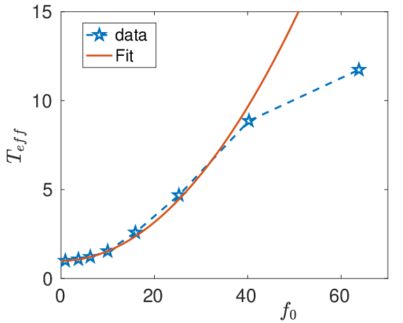
In terms of an effective temperature , as defined in [39], we expect a quadratic increase of with . It was found in [48] that for large , grows more slowly than the predicted quadratic increase (Fig. S3) [39], and this deviation was attributed to activity-induced phase-separation. We leave it for a future study to explore the properties of activity-driven jamming in dense assemblies of active particles.
We can also compare the fragility parameter evaluated in the theory and simulations (Fig. 3b). We again see fair agreement for small and , and a clear deviation between theory and simulation data for larger and larger , as discussed above. Within this model, both and decrease as increases. Thus, fluidises the system and makes it a stronger glass former, similar to varying .
Next we consider Model 2, where and are given by Eqs. (12) and (13). We set a constant and show the behaviour of as a function of as we increase (Fig. 4a). At any value of , we see that increases monotonically as we increase . Thus, promotes glassy behaviour in the active system in the sense that larger drives the system more towards the glassy state, as found in [25]. To display the behaviour of as a function of , we show the Angell plot [52] (Fig. 3b). We find that the curves depart further from the Arrhenius behaviour as increases, which means fragility increases with . From our theory, we obtain that the effective Kauzmann temperature, , glass transition temperature, , and fragility, , all increase with when remains constant. For a quantitative comparison of our theory with simulation data of [25], we rewrite Eq. (13) as in [39] (in the athermal case):
| (17) |
where we have set to unity. Since the dynamics of the system in [25] is a result of activity alone, becomes a function of , and we fit a value of for each value of , as was done in [25] (see Fig. S4 [39]). Note that determines only the large limit, while our model gives precise prediction for the behaviour in the limit of small , approaching the glassy regime. We compare our theoretical results to the data of [25] in Fig. 4(c) using: , and . We also obtained the data for fragility from Fig. 11(b) of [25] and fit it with our theoretical prediction for this model: , with and (Fig. 4d). Our theory predicts that saturates at large (Fig. 4(d) inset). Irrespective of the detailed behaviour, the point is that this system becomes more fragile as increases. This is opposite to the behaviour of Model 1 (at small ). This is also different from the trend shown on increasing within this model.

Discussion
We have developed an RFOT theory for active glasses, by proposing an analytic expression for the active contribution to the configurational entropy, using an effective medium approach that involves the dynamics of a typical active particle within a caging potential. It will be interesting to explore, in future simulations, the extent of validity of this single-particle approach and the relation between the effective parameters of this single-particle theory and the many-body properties of the system, such as the density and inter-particle correlations. While our effective-medium, single-particle model captures the dependence of the mean relaxation time on the activity parameters rather well, it shows deviations at large activities where activity-induced phase-separation and jamming occur. Our theory should be viewed as a first step towards a more rigorous analytical treatment of active glasses.
While we have approximated the effects of activity by a change in the potential energy, it is also possible to define an effective temperature that describes, in an approximate way, the effects of activity. For example, Eq. (9) can be interpreted as changing the temperature to , which implies that the effective temperature increases quadratically with . This is similar to the results reported in [48] which defined an effective temperature from a calculation of the entropy of the active system. Both here (Fig. 3) and in [48], there are deviations from the model at large active forces [39].
What are the implications of our results for cell or tissues that show glassy behaviour? To address this, we need to know the statistical nature of the active fluctuations in these systems. In cells, activity is often realised in the form of active stresses generated by ATP-driven motor proteins that bind/unbind onto an isotropic cytoskeleton (chemical energy transduced per ATP molecule under physiological conditions is kBT). The effective temperature estimated from fluctuations [53, 54] in the active stress arising from independent motors is proportional to , where is the activity correlation time of the force generators [55]. This is precisely of the form Eq. (9) obtained from Model 1, following which we would expect that higher ATP decreases the fragility, driving the system towards a strong glass former, and that activity, controlled through either or , would always fluidise the system. This prediction agrees with early experiments [8, 11] and confirmed in a recent microrheology study [56] of the cytoplasm of a variety of cells, that shows strong glassy behaviour in wild type, which becomes more fragile upon ATP depletion.
Beyond biology, active glasses present a challenge to physics theory, with the main advances in this field relying so far on numerical simulations. Refs. [18, 25] have produced data indicating the opposite roles of the active parameters. Our model provides analytic expressions that give excellent description of available numerical simulation results, and resolves the apparent contradiction between the effects of (or ) and . Since our theory is based on an effective medium approach for the dynamics of a caged active particle, we believe our qualitative results are likely to be independent of the precise form of the inter-particle interactions. Our theory could then be made to confront precision experiments in synthetic systems [26], where the active forces and persistence time can be controlled independently.
.1 Acknowledgements
We thank S. Ramaswamy, P. G. Wolynes and S. Sastry for useful discussions. SKN thanks Koshland foundations for funding through a senior postdoctoral fellowship. RM acknowledge CSIR for financial help and Simons Centre at NCBS for computational resources and hospitality.
References
- [1] S. Ramaswamy, Annu. Rev. Condens. Matter Phys. 1, 323 (2010).
- [2] M. C. Marchetti, J. F. Joanny, S. Ramaswamy, T. B. Liverpool, J. Prost, M. Rao, and R. A. Simha, Rev. Mod. Phys. 85, 1143 (2013).
- [3] J. Prost, F. Jülicher, and J. F. Joanny, Nat. Phys. 11, 111 (2015).
- [4] R. Dreyfus, J. Baudry, M. L. Roper, M. Fermigier, H. A. Stone, and J. Bibette, Nature 437, 862 (2005).
- [5] J. Palacci, S. Sacanna, A. P. S. D. J. Pine, and P. M. Chaikin, Science 339, 936 (2013).
- [6] N. Kumar, H. Soni, S. Ramaswamy, and A. K. Sood, Nat. Comm. 5, 4688 (2014).
- [7] O. Dauchot, G. Marty, and G. Biroli, Phys. Rev. Lett. 95, 265701 (2005).
- [8] E. H. Zhou, X. Trepat, C. Y. Park, G. Lenormand, M. N. Oliver, S. M. Mijailovich, C. Hardin, D. A. Weitz, J. P. Butler, and J. J. Fredberg, Proc. Natl. Acad. Sci. (USA) 106, 10632 (2009).
- [9] T. E. Angelini, E. Hannezo, X. Trepat, M. Marquez, J. J. Fredberg, and D. A. Weitz, Proc. Natl. Acad. Sci. (USA) 108, 4717 (2011).
- [10] S. Garcia, E. Hannezo, J. Elgeti, J. F. Joanny, P. Silberzan, and N. S. Gov, Proc. Natl. Acad. Sci. (USA) 112, 15314 (2015).
- [11] M. Sadati, A. Nourhani, J. J. Fredberg, and N. T. Qazvini, WIREs Syst. Biol. Med. 6, 137 (2014).
- [12] B. R. Parry, I. V. Surovtsev, M. T. Cabenn, C. S. O’Hern, E. R. Dufresne, and C. Jacobs-Wagner, Cell 156, 183 (2014).
- [13] N. Gravish, G. Gold, A. Zangwill, M. A. D. Goodisman, and D. I. Goldman, Soft Matter 11, 6552 (2015).
- [14] T. Kranz, M. Sperl, and A. Zippelius, Phys. Rev. Lett. 104, 225701 (2010).
- [15] L. Berthier and J. Kurchan, Nat. Phys. 9, 310 (2013).
- [16] R. Ni, M. A. C. Stuart, and M. Dijkstra, Nat. Commun 4, 2704 (2013).
- [17] O. Chepizhko and F. Peruani, Phys. Rev. Lett. 111, 160604 (2013).
- [18] R. Mandal, P. J. Bhuyan, M. Rao, and C. Dasgupta, Soft Matter 12, 6268 (2016).
- [19] L. Berthier, Phys. Rev. Lett. 112, 220602 (2014).
- [20] D. Bi, J. H. Lopez, J. M. Schwarz, and M. L. Manning, Nat. Phys. 11, 1074 (2015).
- [21] R. Ni, M. A. C. Stuart, M. Dijkstra, and P. G. Bolhuis, Soft Matter 10, 6609 (2014).
- [22] D. Levis and L. Berthier, Europhys. Lett. 111, 60006 (2015).
- [23] F. Ginot, I. Theurkauff, D. Levis, C. Ybert, L. Bocquet, L. Berthier, and C. Cottin-Bizonne, Phys. Rev. X 5, 011004 (2015).
- [24] G. Szamel, Phys. Rev. E 93, 012603 (2016).
- [25] E. Flenner, G. Szamel, and L. Berthier, Soft Matter 12, 7136 (2016).
- [26] C. Bechinger, R. D. Leonardo, H. Löwen, C. Reichhardt, G. Volpe, and G. Volpe, Rev. Mod. Phys. 88, 045006 (2016).
- [27] G. S. Redner, C. G. Wagner, A. Baskaran, and M. F. Hagan, Phys. Rev. Lett. 117, 148002 (2016).
- [28] S. K. Nandi and N. S. Gov, Soft Matter 13, 7609 (2017).
- [29] L. Berthier and G. Biroli, Rev. Mod. Phys. 83, 587 (2011).
- [30] M. K. Nandi, A. Banerjee, S. Sengupta, S. Sastry, and S. M. Bhattacharyya, J. Chem. Phys. 143, 174504 (2015).
- [31] T. R. Kirkpatrick and P. G. Wolynes, Phys. Rev. A 35, 3072 (1987).
- [32] T. R. Kirkpatrick, D. Thirumalai, and P. G. Wolynes, Phys. Rev. A 40, 1045 (1989).
- [33] V. Lubchenko and P. G. Wolynes, Annu. Rev. Phys. Chem. 58, 235 (2007).
- [34] G. Biroli and J. P. Bouchaud, in Structural Glasses and Supercooled Liquids: Theory, Experiment, and Applications, edited by P. G. Wolynes and V. Lubchenko (John Wiley and Sons, Inc., Hoboken, NJ, USA, 2012).
- [35] T. R. Kirkpatrick and D. Thirumalai, Rev. Mod. Phys. 87, 183 (2015).
- [36] X. Xia and P. G. Wolynes, Proc. Natl. Acad. Sci. USA 97, 2990 (2000).
- [37] A. Wisitsorasak and P. G. Wolynes, Proc. Natl. Acad. Sci. USA 109, 16068 (2012).
- [38] P. G. Wolynes, Proc. Natl. Acad. Sci. USA 106, 1353 (2009).
- [39] “See sup. mat.” (URL).
- [40] V. Lubchenko and P. Rabochiy, J. Phys. Chem. B 118, 13744 (2014).
- [41] S. Karmakar, C. Dasgupta, and S. Sastry, Ann. Rev. Cond. Matt. Phys. 5, 255 (2014).
- [42] R. Mandal, P. J. Bhuyan, P. Chaudhuri, M. Rao, and C. Dasgupta, Phys. Rev. E 96, 042605 (2017).
- [43] É. Fodor, C. Nardini, M. E. Cates, J. Tailleur, P. Visco, and F. van Wijland, Phys. Rev. Lett. 117, 038103 (2016a).
- [44] U. M. B. Marconi, C. Maggi, and S. Melchionna, Soft Matter 12, 5727 (2016).
- [45] W. Kauzmann, Chem. Rev. 43, 219 (1948).
- [46] P. G. Wolynes and V. Lubchenko, Structural Glasses and Supercooled Liquids (John Wiley and Sons, Inc., Hoboken, New Jersey, 2012).
- [47] S. Wang and P. G. Wolynes, J. Chem. Phys. 138, 12A521 (2013).
- [48] Z. Preisler and M. Dijkstra, Soft Matter 12, 6043 (2016).
- [49] E. Ben-Isaac, É. Fodor, P. Visco, F. van Wijland, and N. S. Gov, Phys. Rev. E 92, 012716 (2015).
- [50] M. K. Nandi, A. Banerjee, C. Dasgupta, and S. M. Bhattacharyya, Phys. Rev. Lett. (in press) (2017).
- [51] G. E. Uhlenbeck and L. S. Ornstein, Phys. Rev. 36, 823 (1930).
- [52] C. A. Angell, J. Non-Cryst. Solids 131-133, 13 (1991).
- [53] É. Fodor, M. Guo, N. S. Gov, P. Visco, D. A. Weitz, and F. van Wijland, Europhys. Lett. 110, 48005 (2015).
- [54] É. Fodor, W. W. Ahmed, M. Almonacid, M. Bussonnier, N. S. Gov, M. H. Verlhac, T. Betz, P. Visco, and F. van Wijland, Europhys. Lett. 116, 30008 (2016b).
- [55] A. Basu, J. F. Joanny, F. Jülicher, and J. Prost, Eur. Phys. J. E 27, 149 (2008).
- [56] K. Nishizawa, K. Fujiwara, M. Ikenaga, N. Nakajo, M. Yanagisawa, and D. Mizuno, Sci. Rep. 7, 15143 (2017).
- [57] W. Kob and H. C. Andersen, Phys. Rev. Lett. 73, 1376 (1994).
I Supplementary Material
Systems of self-propelled particles, associated with a self-propulsion force, , and a persistence time, , are good models for a large class of active systems, that include living systems, such as a tissue comprising motile cells [1, 2], or an ensemble of ants, fishes or birds [3, 4] and nonliving systems, such as vertically vibrated polar rods [5, 6]. The internal medium of the cell is associated with large effective viscosities owing to molecular overcrowding and hence can exhibit glassy behaviour. Similarly in the context of tissues, the high density of cells can lead to jamming, a quintessential glassy phenomenon. Both these systems undergo a transition to fluidisation initiated by activity, and hence it is important to understand the glassy dynamics of such active systems. In particular, we would like to understand how active fluctuations affect the approach to glassy behaviour in dense assemblies of active self-propelled particles. One of the outcomes of our theoretical study is to highlight the fact that the detailed nature of activity is important in making predictions about the dependence of activity on features of glassiness.
I.1 Challenges in extending Random First Order Transition (RFOT) Theory to an active system
Introducing activity within the basic RFOT picture [7] presents a number of difficulties:
- •
Active systems are inevitably out of equilibrium and it is not clear how far an extension of a theory that is based on equilibrium thermodynamics is going to be valid.
- •
As the term ‘active system’ describes a diverse class of systems, where activity plays significantly different roles in different systems, a unified description is unrealistic at present.
- •
Configurational entropy density, , and the surface mismatch energy play the major roles within RFOT phenomenology and the precise nature how activity affects these quantities is not known. However, see [8] for results on the entropy of active systems in the dilute limit, i.e., away from the glassy regime.
- •
It is not clear if the basic mosaic picture will survive under activity.
Here we have extended the RFOT theory of conventional glasses to include the effects of activity in a minimal way. Since active systems are manifestly out of equilibrium, we must first find a physically reasonable definition of the configurational entropy for such systems. The configurational entropy of passive thermal systems is usually defined in terms of the multiplicity of the local minima of the potential energy (“inherent structures”) whose basins of interaction are visited by the system at a particular temperature . Here, we continue to use the same definition of the configurational entropy for active systems. Particle configurations in a steady state of an active systems can be used as starting points of a minimisation procedure to locate a set of inherent structures characteristic to the steady state being considered. The multiplicity of inherent structures obtained this way would be different from that of the inherent structures obtained for an identical system without activity at the same temperature. Therefore, the temperature dependence of the configurational entropy of an active system would be different from that for its passive counterpart. We have obtained the average energy, , of inherent structures as a function of activity strength for the model of Ref. [9] and find that increases with at a fixed temperature as shown in Fig. S1. In the next section, we present the details of how we compute the activity corrections to the configurational entropy within a specific model of a system of self-propelled particles.

I.2 Active contribution to configurational entropy
Following [10, 11, 12] and the discussion above, we take the configurational entropy density to depend on the many-body potential at temperature .
We start with the overdamped dynamics of the system of passive particles, given by,
| (S1) |
where is the position of the -th particle, is the many-body potential experienced by particle and is the thermal noise (gaussian, white noise with zero mean). Defining the full many-body potential as , Refs. [10, 11, 12, 13] would suggest that the configuration entropy depends on the steady state profile of this : (where is understood to be averaged over the steady state distribution corresponding to Eq. (S1)). At this stage, we need not know how to compute this; all we need is that this is somehow given. With this in hand, we discuss an effective medium approach that goes into the calculation of the activity corrected configuration entropy density needed for the active version of the RFOT theory described in the main text.
To this end, we first note that the corresponding dynamical equation for active self-propelling particles is,
| (S2) |
where is an active noise taken to be exponentially correlated in time, with zero mean. One can interpret the above equation [14, 15] as modifying the effective many-body potential experienced by particle by,
| (S3) |
The corresponding configurational entropy density for the active system is , which we expand in a Volterra series (or a functional Taylor series) as,
| (S4) | |||||
In what follows, we will retain only the first term, assuming is small. However, evaluating this first-order correction, even approximately, poses a problem.
Effective-medium approach : To proceed we first approximate the above many-body dynamics by the dynamics of a typical self-propelled particle with coordinate moving in an effective caging potential , where the collective variable , is assumed to evolve much slower than , i.e., over a time scale equal to or greater than the -relaxation time, . Here we take the caging potential to be harmonic and static, the overdamped Langevin dynamics is then given by
| (S5) |
where is the effective particle friction coefficient. This assumes that .
We will now approximate the first-order correction in Eq. (S4) by , where , an active fragility parameter, and is an average over the steady state distribution corresponding to Eq. (S5). This parameter measures the sensitivity of the configurational entropy to changes in the potential or alternatively, the active force. For simplicity, we will take it to be a constant fit parameter (although there is no apriori justification for this). The term can be easily evaluated by solving the corresponding Fokker-Planck equation, which we will now do for the two models of active forcing described in the main text.
The motivation for identifying the active correction to the configurational entropy with the change in potential energy of a trapped active particle, can be as follows [16]: due to activity the particle explores the space around it to a larger extent, and this can be quantified by the change in potential energy, similar to an “effective temperature” (see below).
Model 1: , where is the average strength and is the persistence of the active noise.
With this noise statistics, Eq. (S5) written for a harmonic caging potential in one dimension, is equivalent to the following Ornstein-Uhlenbeck process [17, 9],
| (S6) | |||||
| (S7) |
where is the spring constant of the harmonic potential, and the noise has zero mean and is delta-correlated and white : and . The calculation below is qualitatively identical to the case with fixed active force amplitude [18].
The corresponding Fokker-Planck equation for the joint probability distribution, , is [19],
| (S8) |
whose steady state is easily seen to be [19],
| (S9) |
with , and , and is the normalization factor.
This can be simply integrated over , to obtain the marginal distribution,
| (S10) |
which has a Boltzmann form, , with an effective temperature [18],
| (S11) |
Using the steady state joint probability distribution , we can show that for Model 1,
| (S12) |
Model 2: , where is the persistence of the active noise.
With this noise statistics, Eq. (S5) for a harmonic caging potential, is equivalent to the following Ornstein-Uhlenbeck process [17, 9],
| (S13) | |||||
| (S14) |
where the noise has zero mean and is delta-correlated, white : and .
The corresponding Fokker-Planck equation for the joint probability distribution, , is [19],
| (S15) |
whose steady state solution is,
| (S16) |
with , and . The marginal distribution is,
| (S17) |
which again has a Boltzmann form, with an effective temperature
| (S18) |
Using the steady state joint probability distribution , we can show that for Model 2,
| (S19) |
I.3 Comparison with recent simulation in terms of effective temperature ()

Within the effective medium approach outlined above, the steady state distribution always has a Boltzmann form, and hence we can assign an effective temperature, as in Eqs. (S11) and (S18). Such effective temperature descriptions have been discussed in [20, 17, 21, 22, 23, 8, 24, 25]. This is fortuitous and may not always be possible [14], especially in active dense many-body systems.
We therefore compare the effective temperature definition in a many-body active system [8], with the effective medium approach. Ref. [8] has proposed a method to calculate the entropy of an active system consisting of Brownian spheres and show that active systems can be mapped to equilibrium systems with a many-particle distribution function akin to Boltzmann distribution, but characterised by an effective temperature. Ref. [8] considers the coefficient of rotational Brownian motion, , as a measure of persistence, . Using Eq. (S11) we obtain in terms of and , the self-propulsion velocity, as
| (S20) |
where is the equilibrium temperature (set to unity) and and are two constants. We have included the factor , as defined in [8], in above since remained constant in the simulation. We obtain the constant parameters and by fitting Eq. (S20) with the data corresponding to in Fig. 4(b) in [8] and show the behavior of Eq. (S20) along with the data of [8] in Fig. S2. Note that the theoretical analysis in [8] was done in the limit . This comparison shows the consistency of our approximation.
We have found that our theory deviates from the simulation results at large activity (Fig. 3 in the paper). When activity becomes large, the system is driven far away from equilibrium and our effective medium approach breaks down. Ref. [48] also finds such a deviation; we have plotted in Fig. S3 the data from Fig. 5(b) of [8], and the fit with our model (Eq. S20) with being a fitting parameter for small .
Simulation model
We follow the simulation strategy as detailed in [18]. We perform a molecular-dynamics (MD) simulation of a Kob-Andersen binary mixture [57] of A and B-type particles in the ratio (80:20) interacting via a Lennard-Jones pair potential,
| (S21) |
where is the distance between two particles and indices . The units of length and energy are determined by setting and . The rest of the parameter values are taken to be: , , , . The mass of the particles are and the overall number density of the system is . The interaction potential is cutoff at and it is smoothed with a quadratic function so that both the energy and forces are continuous at the . The particles follow Newton’s laws; the equations of motion are integrated by employing the velocity version of the Verlet algorithm.
A fraction of B-type particles () are subject to a propulsion force, whilst keeping the rest of the particles passive (here, we set ). Self-propulsion forces of the form are randomly assigned to the active B-particles, with chosen randomly to have values , so as to conserve the net momentum of the system. The active particles are driven in the directions of for a persistence time , the directions of are then randomised by choosing a different set of . We have checked that the dynamics driven by this 8-state clock realisation of the random propulsion forces, has the same qualitative features as a continuous O(3) realisation. Simulations here are for particles; we have checked that finite size effects are negligible.
Dynamical quantitites
The slow dynamics is captured by the two-point correlation function, , defined as:
| (S22) |
where,
Here the is an average over number of particles and time origin . The parameter is associated with the typical amplitude of vibrational motion of the particles. We have used for our analyses. The decay of in time is a measure of the dynamical slowing down and defines the -relaxation time , via . The -relaxation time at different temperatures for a given can be fitted to the Vogel-Fulcher-Tamman (VFT) form,
| (S23) |
where is the relaxation time at high temperatures and is the kinetic fragility. The relaxation time extrapolates to infinity at , the putative glass transition temperature.
I.4 Details for the results
Within Model 1, we have the equations governing the most probable mosaic length scale, , and relaxation time as
| (S24) | ||||
| (S25) |
To compare with simulation data, we obtain the data from Fig. 8 of Ref. [9] and write Eq. (S25) as
| (S26) |
and obtain different constants through fitting the above equation with a particular data corresponding to . In principle, we could also obtain these parameters from the detailed microscopic knowledge of the system that we didn’t attempt here. The excellent agreement between the theoretical predictions and simulation data shows that our theory captures the basic physics of the system. In this work we have assumed to be same as , the surface mismatch energy of a passive system, for simplicity. We also tried different forms for . When we considered the amplitude of to be small, the detailed form of didn’t alter the results qualitatively which is expected from Eq. (4). We obtained the best fit with a vanishing as shown in Figs. 2(c) and (d). It is possible that has a non-trivial dependence on activity, but it is sub-dominant for the model we considered such that it doesn’t play a major role in the glassy properties of the system.

For a quantitative comparison with simulation data when activity is controlled through , we compare our theory with Ref. [26], which considers an athermal system of self-propelled particles where the dynamics of the system solely comes from activity. The active force in the simulation of [26] obeys
| (S27) |
where is a Gaussian white noise with zero mean and variance (See Eq. 2 in Ref. [26]). With this active force that belongs to Model 2 in our classification and therefore using Eq. (S19) we obtain the relaxation time as
| (S28) |
where we have set to unity. Since Ref. [26] considers a system where temperature doesn’t play any role, we have set . We obtain the data for relaxation time from Fig. 6 of Ref. [26] for , , and . As the dynamics solely arises due to activity, becomes a function of when dominates the dynamics. Since is not large, we neglect the second-order term in in the denominator of Eq. (S28) and through fitting we obtain , , and and , , and for , , ans respectively. These values of are approximately times higher than the value of obtained in [26] through the fitting of a different equation and a different temperature regime, hence, it’s not surprising that their absolute values are different, however, we find that they are proportional. In the inset of Fig. S4 we show as obtained in Ref. [26] by the solid line, obtained by our fit by and we plot these values scaled by 2.5 as shown by . We show the comparison of our theory with the simulation data in Fig. S4. In the main paper, we chose to present the same plot as as a function of as we wanted to emphasise the dependence of on in the low-temperature regime.
References
- [1] J. Prost, F. Jülicher, and J. F. Joanny, Nat. Phys. 11, 111 (2015).
- [2] S. Garcia, E. Hannezo, J. Elgeti, J. F. Joanny, P. Silberzan, and N. S. Gov, Proc. Natl. Acad. Sci. (USA) 112, 15314 (2015).
- [3] S. Ramaswamy, Annu. Rev. Condens. Matter Phys. 1, 323 (2010).
- [4] N. Gravish, G. Gold, A. Zangwill, M. A. D. Goodisman, and D. I. Goldman, Soft Matter 11, 6552 (2015).
- [5] N. Kumar, H. Soni, S. Ramaswamy, and A. K. Sood, Nat. Comm. 5, 4688 (2014).
- [6] O. Dauchot, G. Marty, and G. Biroli, Phys. Rev. Lett. 95, 265701 (2005).
- [7] T. R. Kirkpatrick, D. Thirumalai, and P. G. Wolynes, Phys. Rev. A 40, 1045 (1989).
- [8] Z. Preisler and M. Dijkstra, Soft Matter 12, 6043 (2016).
- [9] R. Mandal, P. J. Bhuyan, M. Rao, and C. Dasgupta, Soft Matter 12, 6268 (2016).
- [10] X. Xia and P. G. Wolynes, Proc. Natl. Acad. Sci. (USA) 97, 2990 (2000).
- [11] S. Sastry, Nature 409, 164 (2001).
- [12] L. Berthier and D. Coslovich, Proc. Natl. Acad. Sci. (USA) 111, 11668 (2014).
- [13] S. Sengupta, F. Vasconcelos, F. Affouard, and S. Sastry, J. Chem. Phys. 135, 194503 (2011).
- [14] É. Fodor, C. Nardini, M. E. Cates, J. Tailleur, P. Visco, and F. van Wijland, Phys. Rev. Lett. 117, 038103 (2016).
- [15] U. M. B. Marconi, C. Maggi, and S. Melchionna, Soft Matter 12, 5727 (2016).
- [16] S. K. Nandi and N. S. Gov, Soft Matter 13, 7609 (2017).
- [17] G. Szamel, Phys. Rev. E 90, 012111 (2014).
- [18] E. Ben-Isaac, É. Fodor, P. Visco, F. van Wijland, and N. S. Gov, Phys. Rev. E 92, 012716 (2015).
- [19] C. W. Gardiner, Stochastic Methods: A Handbook for the Natural and Social Sciences, 4th ed. (Springer, 2009).
- [20] D. Loi, S. Mossa, and L. F. Cugliandolo, Soft Matter 7, 3726 (2011).
- [21] S. Wang and P. G. Wolynes, J. Chem. Phys. 135, 051101 (2011).
- [22] E. Ben-Isaac, Y. Park, G. Popescu, F. L. H. Brown, N. S. Gov, and Y. Shokef, Phys. Rev. Lett. 106, 238103 (2011).
- [23] T. Shen and P. G. Wolynes, Proc. Natl. Acad. Sci. (USA) 101, 8547 (8547).
- [24] G. S. Redner, A. Baskaran, and M. F. Hagan, Phys. Rev. E 88, 012305 (2013).
- [25] G. S. Redner, C. G. Wagner, A. Baskaran, and M. F. Hagan, Phys. Rev. Lett. 117, 148002 (2016).
- [26] E. Flenner, G. Szamel, and L. Berthier, Soft Matter 12, 7136 (2016).