Hardware Based Projection onto
The Parity Polytope and Probability Simplex
Abstract
This paper is concerned with the adaptation to hardware of methods for Euclidean norm projections onto the parity polytope and probability simplex. We first refine recent efforts to develop efficient methods of projection onto the parity polytope. Our resulting algorithm can be configured to have either average computational complexity or worst case complexity on a serial processor where is the dimension of projection space. We show how to adapt our projection routine to hardware. Our projection method uses a sub-routine that involves another Euclidean projection; onto the probability simplex. We therefore explain how to adapt to hardware a well know simplex projection algorithm. The hardware implementations of both projection algorithms achieve area scalings of at a delay of . Finally, we present numerical results in which we evaluate the fixed-point accuracy and resource scaling of these algorithms when targeting a modern FPGA.
I Introduction
The need for hardware-compatible algorithms that can project onto the parity polytope, and onto the probability simplex, is motivated by linear program (LP) decoding techniques for LDPC codes. LP decoding of error-correcting codes is a relatively new concept that originated in Jon Feldman’s Ph.D. [1, 2]. Since then, much work has been done to make this approach more appealing to practical implementation. For example, progress has been made by approximating the LP decoding problem by a solver that has linear complexity in blocklength [3, 4]. Additionally, [5] showed how the complexity and performance of LP decoding can be improved by starting with a simple linear program and adaptively adding constraints. More recently, [6] applied the ADMM decomposition technique from [7] to LP decoding. This decomposition gives rise to a distributed algorithm which relies heavily on parity polytope projections. We will see that projection onto the probability simplex plays a integral role in parity polytope projections.
Hardware implementation of these projection algorithms are needed in order for ADMM decoding to be practical. This is especially true for applications with stringent reliability requirements and high data rates (e.g., optical transport). These are also the applications for which the theoretical guarantees of LP decoding are especially attractive. Therefore, this study is the first step in determining whether or not ADMM is a commercially viable LP decoding algorithm.
First, we review the state of available projection techniques in Section II. Then we evaluate and choose algorithms that are suitable for hardware implementation in Section III. For projecting onto the parity polytope, we develop a new technique based on previous approaches, but more compatible with hardware. The correctness of this method is proved. Section IV is dedicated to the adaptation of the algorithms to hardware. Finally, we implement the selected projection algorithms in Verilog and synthesize them for an Altera Stratix V FPGA. This allows us to investigate fixed-point precision effects as well as resource scaling. Findings are reported in Section V.
Because of the spreading use of FPGA and hardware acceleration in computing, we anticipate the developments and experiments in this paper will be of interest to fields other than error-correction coding (e.g., optimization and machine learning). Therefore, we present our results in full generality, outside the specific context of error-correction.
II Background
II-A Projecting onto the Parity Polytope
As visualized in Fig. 1, the parity polytope is defined as the convex hull of all even weight vertices of the unit hyper-cube, i.e.,

The parity polytope is a polyhedron. Therefore, as discussed in [6], projecting a point onto is a quadratic program,
| (1) |
where (Euclidean) projection onto the set is denoted .
A computationally tractable approach to solving (1) was given in [6]. The approach involves a “two-slice” characteristic of points in the parity polytope. These points can be represented as a convex combination of binary vectors with weight or for some even integer . The authors show that the projection is invariant to the ordering of input vector components. By first applying a sort, finding the two-slice representation of the projection is reduced to an optimization over a piecewise linear function that has complexity. The two-slice approach is limited by the sorting and desorting of vector components, which gives it a computational complexity of .
Zhang and Siegel developed a more efficient projection algorithm in [8]. Their algorithm first determines the facet of the parity polytope on which the projection lies. They then project onto said facet. Determining the correct parity polytope facet is achieved by employing the authors’ “cut search” algorithm, fully described in [9]. To project a point onto the facet found, the authors use the same optimization over a piecewise linear function described in [6]. This method is less complex than [6] because the sort and desort operations in [6] are replaced by the cut search operation. However, due to this change a sort is still required in solving the piecewise linear optimization problem, resulting in the same order computational complexity .
Even more recently, another projection algorithm was proposed in [10]. The first improvement is to use a partial sort on input vector components instead of a full sort (as in [6]) to obtain the same result. Second, the authors show that the projection’s two-slice representation can be computed via a projection onto the probability simplex. Both of these operations have expected complexity that is linear in dimension, giving the entire projection algorithm an expected computational complexity of . However, worst case complexity is quadratic.
II-B Projecting onto the Probability Simplex
The probability simplex is defined as the set of all positive vectors whose components sum to one. Precisely:
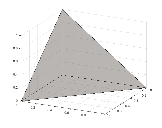
Fig. 2 visualizes the probability simplex in . Similar to the parity polytope, projection onto this set is a quadratic program:
An excellent reference for projection onto the probability simplex is found in [11]. The authors first develop a method for simplex projection that uses a sorting of the input components. The complexity is . Next, the authors develop a linear expected complexity (quadratic worst case complexity) algorithm that performs similar calculations to their first approach in an iterative manner. Additionally, the authors describe how to use projection onto the probability simplex to compute projection onto the -ball.
III Algorithmic Adaptation
Before tackling the hardware implementation of the projection algorithms, we evaluate the techniques discussed in Section II for their hardware compatibility. Criteria we use include computational complexity, delay, parallizability, and input invariance. By input invariance we mean that the same operations are performed regardless of input values.
III-A Adapting the Parity Polytope Projection
The parity polytope projection routines specified in [6] and [8] contain the same overall structure and computational complexity which scales well. The drawback of these algorithms is their iterative nature. This results in high delay, low potential for parallelization, and input dependence.
The projection routine from [10] has good overall structure and excellent computational complexity. However, we believe it is difficult to adapt this algorithm’s average complexity to hardware. The technique relies on a partial sort for which we have not found a general hardware technique (except to implement a partial sort via a full sort). Additionally, the simplex projection suggested in [10] is poorly suited for hardware. We will see another routine for the latter task that maps well to hardware.
Each of the algorithms discussed above has its own merits, yet we believe none is suitable for hardware adaptation. Therefore we introduce a novel approach by combining two of the techniques. This new method is similar to that presented in [10]. However, we employ the cut search method used in [8] to identify which facet to project onto. We then perform the projection using a probability simplex projection. Doing this avoids the partial sort and replaces it with a guaranteed linear complexity component. Algorithm 1 describes this method in full. Definition 1 provides a similarity transformation that is used in the proposed algorithm.
Definition 1.
Given a vector and a vector , we define the operator as
where . Note that this is very similar to Definition 2 in [10].
Input:
Output:
We demonstrate the correctness of the algorithm by partitioning the possible inputs into two cases. The first case is when the unit cube projection of the algorithm input is in the parity polytope. i.e., . The second case covers all other inputs.
As we will see, Theorem 1 (below) provides the test to differentiate between the two cases. This theorem is used on line 8 of Algorithm 1. First we introduce a lemma that aids in the development of the theorem.
Lemma 1.
Given and ,
| (2) |
Proof.
First note that both and are component-wise operators. Therefore the lemma can be proved by examining a single component. We now consider the cases of . When , then . This gives equality in (2) for all cases of .
When , we consider three cases for . First, if , the left hand side of (2) becomes . Also, will be greater than , making the right hand side . Second, if , the left hand side becomes . Also, will be less than , making the right hand side . Finally, if the left hand side becomes . The right hand side also reduces to since is between and . ∎
Theorem 1.
Given and as calculated in Algorithm 1,
Proof.
Since the parity polytope is a subset of the unit cube, we return when satisfies Theorem 1 (line 9 of Algorithm 1). When does not satisfy Theorem 1, we find the projection onto the parity polytope via a projection onto the probability simplex (lines 11 and 12 of Algorithm 1). The correctness of this method is given by Theorem 2 below.
Theorem 2.
Given such that and as calculated in Algorithm 1,
Proof.
We start with optimization problem (18) presented in [8]. We then apply the change of variable . This gives us a projection onto the probability simplex. ∎
This projection algorithm can be configured to have average complexity or worst case complexity depending on the implementation of as outlined in Section II-B.
III-B Adapting the Probability Simplex Projection
We considered both methods presented in [11] for hardware based projection onto the probability simplex. One has linear expected complexity, but is highly input dependent and iterative. This makes it a bad candidate for hardware. Because of this, we use the other method from [11] which has computational complexity. It is logical that this complexity is necessary since the expected linear time algorithm performs the same computations as the algorithm while avoiding, or combining, operations when possible. It is exactly this characteristic that makes the algorithm unsuitable for hardware. The technique we use is described fully by Algorithm 2, below. As can be guessed, the descending sort operation sorts the vector components into descending order.
Input:
Output:
We have not made any modifications to the statement of this algorithm in [11].
IV Hardware Implementation
We now discuss the implementation and architectural choices we made to realize, in hardware, a routine that projects onto the parity polytope. To measure the efficiency of our implementation we consider the FPGA area usage of the synthesized algorithm, as well as delay.
We make a comment regarding the fixed-point representation we use in our implementations. Within certain sub-modules of the projection routine we provide enough additional dynamic range to avoid overflow. Then, after the projection is computed, excess bits are truncated to deliver an output with the same bit width as the projection module input.
IV-A Implementing the Parity Polytope Projection
The majority of steps in Algorithm 1 comprise straightforward operations that map directly to parallelizable hardware constructs with linear complexity and constant delay. There are two exceptions to this: the simplex projection and the argmin operation. The simplex projection will be discussed in a subsequent section. The argmin operation on line 4 of Algorithm 1 warrants an explanation, as it does not have constant delay.
IV-A1 Argmin
The output of the argmin module is the minimum along with a one-hot indicator vector that indicates which element of the input vector was minimal. This calculation is realized using a min-tree where each node recursively calls two argmin operations. Using the two minima received, the indicator vector of the higher value is zeroed and concatenated with the indicator vector of the lower value. This construction has linear complexity and logarithmic delay.
IV-B Implementing the Probability Simplex Projection
We now explain the various operations in the probability simplex projection that do not map trivially to hardware implementation. We will see in this section that the realization in hardware increases the computation complexity (as measured by area usage) of the projections from to . This increase is due to a parallel implementation of the sort operation.
IV-B1 Sort
As mentioned, sorting is a key aspect of the projection algorithm developed in [6]. Sorting is relevant due to the permutation symmetry of the parity polytope. Unfortunately, most sorting methods are highly input dependent. For example, quick-sort makes recursive calls of varying size depending on the input data and the pivot value. We instead use sorting networks. These are circuits composed of compare and swap modules that perform the same operations regardless of the input data. Sorting networks are explained in detail in [12].
Our construction relies on delay-optimal sorting networks for dimension 16 or less, specified in [12]. For larger dimensions we use Batcher’s odd-even merge-sort (also discussed in [12]) with recursive calls to the optimal sorting networks when possible. Batcher’s sort has the same recursive structure as a standard merge sort. However, the merging operation is performed in a clever manner that is input invariant. The price of invariance is an increase in area to with a delay of . We comment that another sorting network, the AKS network, scales better in dimension than our approach. However, according to [12], AKS networks are completely impractical in any application.
IV-B2 Prefix Sum
Prefix sum refers to the sum operation on line 2 in Algorithm 2 whereby all partial sums of the sorted vector are obtained. Performing this operation efficiently in serial is straightforward. It is less obvious that a parallel algorithm can perform this computation with logarithmic delay and linear complexity. However, several such algorithms indeed do exist and have been tested [13] for their hardware compatibility in an FPGA. In [13] the construction of Ladner and Fischer [14] scales best with respect to delay and area. We therefore use their method. It should be noted that this method achieves the minimum possible delay of add operations on its critical path.
IV-B3 Max Index
Max index is the operation performed on line 3 of Algorithm 2. The max index module takes as input a bit vector of length where the high bits represent the set of indices from which we want to select the maximum. The module creates a one-hot bit vector where the high bit in the output corresponds to the largest index high bit in the input. We can see that in order for the output bit to be high, the input bit must be high and all input bits above it must be low. Writing out the Boolean expression for each output bit, we can observe that this module is a prefix operation having almost identical structure to the previously mentioned prefix sum. We take the same approach as already described for prefix sum. The difference being the use of logical AND operations instead of additions.
Now that we have addressed how non-trivial operations will be mapped into hardware, we can evaluate the complexity of the projection hardware module. The sort operation is the most expensive module to implement. It gives the entire parity polytope projection module an area complexity of with delay.
V Results
V-A Fixed Point Effects
V-A1 Projections in the Unit Cube
The objective of our first experiment is to determine the accuracy of the proposed projection algorithms when implemented in fixed-point. To test accuracy, we generate vectors uniformly at random from the three dimensional unit cube. We then project the vectors onto the parity polytope and probability simplex using varying degrees of fixed-point accuracy.
To quantify the degradation with bit width, we start by generating double precision random vectors in MATLAB. We then apply a uniform quantizer to these vectors. This creates the fixed-point representation of the points to be projected. The fixed-point representation of the input and output vectors were both given 1 sign bit, 0 integer bits, and a varying number of fraction bits. This is because the absolute value of vector components will not exceed 1. These fixed-point vectors were then projected onto the parity polytope and probability simplex using the Verilog modules we created. As a point of comparison, the double precision input vectors were also projected onto the parity polytope and probability simplex. This latter projection was performed in MATLAB using double precision arithmetic.
The average dimension normalized squared error is shown in Fig. 3 for the quantized input, for the fixed-point parity polytope projection, and for the fixed-point probability simplex projection. The error measurement for each curve is relative to the corresponding double precision calculation. The fixed-point width is varied from 2 to 16 bits, corresponding to a number of fraction bits varying from 1 to 15.

As would be expected for uniform quantization over a fixed range, the input error decreases exponentially (recall the 6dB/bit SNR rule of thumb). We also find that the projection error decreases exponentially in bit width. We believe the zig-zag in the projection error plot results from the fixed-point representation of in line 2 of Algorithm 2. Every second bit that is added to the binary representation of gives a disproportionate amount of accuracy since the representation is alternating s and s (i.e., ).
The general shape of the curve - the exponential decrease in error - was seen for all trials on all dimensions (we simulated projections for various dimensions up to ). These results are not shown here since the zig-zagging effect is not as pronounced when there are more fractions from line 2 of Algorithm 2 that cannot be represented exactly.
V-A2 Gaussian Projections
The second fixed-point precision experiment investigates the trade-off between dynamic range and accuracy when projecting onto the parity polytope. Our approach is similar to the first experiment except the random input vector components have a normal distribution with mean zero and variance of 16.
Fig. 4 shows how the accuracy of various fixed-point representations compare to double precision projections. The input representation of all trials contains 1 sign sign bit. Each curve represents a different number of integer bits for the input representation. The x-axis shows the total fixed-point width. It is varied by changing the number of fraction bits in the input representation. Every output representation is composed of 1 sign bit, 1 integer bit, and a varying number of fraction bits giving the same fixed-point width as the input. We can see that the various error curves in Fig. 4 start at different locations. This is because each representation requires a different minimum width to accommodate its sign bit and integer bits.

For representations having 0, 1, or 2 integer bits in the input fixed-point representation, there is a small period of exponential decrease in error. This is followed by a saturation regime due to a lack of dynamic range. The 2 integer bit trial was the only curve with non-trivial error bars. Therefore they are displayed.
The 3 and 4 integer bit representations overcome the lack of dynamic range. This is indicated by the exponential decrease in error across the entire plotted range. We also observe that 3 integer bits performs better than 4 for all visible widths. This indicates that, for this class of input vectors, an extra bit is better spent on accuracy than on dynamic range.
Finally, we can also see what the optimal representation format is with regard to squared error. Below a fixed-point width of 8 bits, 2 integer bits is the best choice. Bits are better spent on accuracy than on dynamic range. However, when more than 8 bits are used in the representation, only having 2 integer bits results in a saturation regime, making the 3 integer bit representation the better choice.
V-B Resource Scaling
We also synthesized the circuits in question for a range of dimensions to obtain real measurements of area and delay scaling. This synthesis was performed for an Altera Stratix V FPGA (model 5SGXEA7N2F45C2) which has 234,720 adaptive logic modules. The two projection circuits along with the sorting circuit were configured to have 8 bits of fixed-point precision: 1 sign bit, 1 integer bit, and 6 fraction bits for both input and output. The percentage of logic modules consumed by the synthesized circuits is a meaningful proxy measurement for area. In order to make the measurement even more meaningful, we disabled the synthesizer’s ability to map arithmetic operations to dedicated DSP blocks.

The area measurements plotted in Fig. 5 make the superlinear area scaling described in Section IV visible. We can also see that all three modules follow similar area curves, indicating that the sort operation is the complexity dominating module. In order to observe practical delay scaling, we measured the critical path delay of the compiled circuits. Keep in mind that these circuits were compiled without any pipelining. Delay measurements are shown in Fig. 6.

Similar to the area experiment, we see that delay measurements roughly follow the scaling predicted in Section IV. In addition, the curves are quite similar. This is further evidence that the sort operation is the delay dominating module. Note also the jumps in area and delay at dimensions that are powers of two in Fig. 5 and Fig. 6. These jumps occur because another layer must be added to the merge sort, emphasizing again the effect sorting has on the projection routines.
VI Conclusion
In this paper, we reviewed two essential optimization problems that have high throughput applications: projection onto the parity polytope and projection onto the probability simplex. Building off previous innovations, we were able to create hardware friendly algorithms to realize these projections. This enabled the creation of fixed-point implementations that were tested and found to have viable error curves and resource footprints.
The next step in our research is to apply these results to decoding error-correcting codes. We believe this will lead to a proof of concept for the LP decoding algorithm proposed in [6]. We also believe that further research into more efficient, hardware compatible, projection algorithms would be extremely useful. This would be especially true if said research yields projection algorithms that completely avoid a sort operation.
References
- [1] J. Feldman, “Decoding error-correcting codes via linear programming,” Ph.D. dissertation, MIT, MA, USA, 2003.
- [2] J. Feldman, M. J. Wainwright, and D. R. Karger, “Using linear programming to decode binary linear codes,” IEEE Trans. Inf. Theory, vol. 51, no. 3, pp. 954–972, Mar. 2005.
- [3] P. O. Vontobel and R. Koetter, “Towards low-complexity linear-programming decoding,” in Proc. 4th Int. Symp. Turbo Codes and Related Topics, Munich, Germany, Apr. 2006, pp. 1–9.
- [4] D. Burshtein, “Iterative approximate linear programming decoding of LDPC codes with linear complexity,” IEEE Trans. Inf. Theory, vol. 55, no. 11, pp. 4835–4859, Nov. 2009.
- [5] M. H. Taghavi and P. H. Siegel, “Adaptive methods for linear programming decoding,” IEEE Trans. Inf. Theory, vol. 54, no. 12, pp. 5396–5410, Nov. 2008.
- [6] S. Barman, X. Liu, S. C. Draper, and B. Recht, “Decomposition methods for large scale LP decoding,” IEEE Trans. Inf. Theory, vol. 59, no. 12, pp. 7870–7886, Dec. 2013.
- [7] S. Boyd, N. Parikh, E. Chu, B. Peleato, and J. Eckstein, “Distributed optimization and statistical learning via the alternating direction method of multipliers,” Machine Learning, vol. 3, no. 1, pp. 1––122, 2011.
- [8] X. Zhang and P. H. Siegel, “Efficient iterative LP decoding of LDPC codes with alternating direction method of multipliers,” in Proc. IEEE Int. Symp. Inf. Theory, Istanbul, Turkey, Jul. 2013, pp. 1501–1505.
- [9] ——, “Adaptive cut generation algorithm for improved linear programming decoding of binary linear codes,” IEEE Trans. Inf. Theory, vol. 58, no. 10, pp. 6581–6594, Oct. 2012.
- [10] G. Zhang, R. Heusdens, and W. B. Kleijn, “Large scale LP decoding with low complexity,” IEEE Commun. Lett., vol. 17, no. 11, pp. 2152–2155, Nov. 2013.
- [11] J. Duchi, S. Shalev-Shwartz, Y. Singer, and T. Chandra, “Efficient projections onto the -ball for learning in high dimensions,” in Proc. Int. Conf. Machine Learning, San Diego, CA, USA, Dec. 2008.
- [12] D. E. Knuth, The Art of Computer Programming: Sorting and Searching, 2nd ed. Redwood City, CA, USA: Addison Wesley Longman, 1998.
- [13] K. Vitoroulis and A. J. Al-Khalili, “Performance of parallel prefix adders implemented with FPGA technology,” in Proc. NEWCAS Workshop, Montreal, Que, Canada, Aug. 2007.
- [14] R. E. Ladner and M. J. Fischer, “Parallel prefix computation,” J. of the ACM, vol. 27, no. 4, pp. 831–838, Oct. 1980.