Stable Interacting $(2+1)d$ Conformal Field Theories at the Boundary of a class of
$(3+1)d$ Symmetry Protected Topological Phases

A symmetry protected topological (SPT) phase [1, 2] must, by definition, have a boundary state with a nontrivial spectrum when the system including the boundary preserves certain global symmetries. Many $(2+1)d$ SPT states can be described with a similar Chern-Simons theory [3] as the quantum Hall states, their $(1+1)d$ boundary states are therefore relatively easy to understand. Thus it is more challenging to understand the $(3+1)d$ SPT states, whose boundary states can have much richer physics under strong interaction. The following three types of $(2+1)d$ states may exist at the boundary of a $(3+1)d$ SPT phase:

1) An ordered phase that spontaneously breaks the global symmetry and hence has degenerate ground states;

2) A $(2+1)d$ topologically ordered phase with topological degeneracy;

3) A stable gapless phase which is described by a conformal field theory (CFT).

Possibilities 1 and 2 have both been studied quite extensively in the last few years, for both fermionic and bosonic SPT states [4, 5, 6, 7, 8, 9, 10], but there is little study about the third possibility, except for the well-known simplest case of noninteracting topological insulators/superconductors. In this work we explore the third possibility of SPT phases: a stable $(2+1)d$ interacting conformal field theory (CFT) at the boundary of a $(3+1)d$ SPT state. This CFT should be stable against any symmetry allowed perturbations, By “stable” we mean that all perturbations allowed by symmetry should be irrelevant (in the renormalization group sense) at this fixed point.

We will take the “standard” field theory description of $(3+1)d$ bosonic SPT states, which is a nonlinear sigma model (NLSM) with a $\Theta$-term in the $(3+1)d$ bulk spacetime. The value $\Theta=2\pi$ corresponds to the stable fixed point of the SPT phase. This formula was used to describe and classify bosonic SPT states in Ref. 9, 11, 12, 10. With $\Theta=2\pi$ in the $(3+1)d$ bulk, the $(2+1)d$ boundary is described by a NLSM with a Wess-Zumino-Witten (WZW) term with level $k=1$. In Ref. 9, 11, 10, the target space of the NLSM was the four dimensional sphere $S^{4}$, a WZW term can be defined based on the fact that the homotopy group $\pi_{4}[S^{4}]=\mathbb{Z}$. Topological phases with the same anomaly as this field theory under various anisotropies were discussed thoroughly in Ref. 9, 10.

The presence of a WZW term is known to drastically change the behavior of the NLSMs in lower dimensions. In particular, in $(0+1)d$ a WZW term may lead to degenerate ground states; in $(1+1)d$ a WZW term drives the NLSM towards a conformally invariant fixed point [13, 14]. An explicit renormalization group (RG) calculation in $(1+1)d$ demonstrates that this fixed point is stable and occurs at a finite value of the NLSM coupling constant [13].

However, unlike these $(1+1)d$ analogues, it is difficult to perform a controlled calculation for NLSMs with a WZW term in $(2+1)d$. There are two standard controlled RG calculations for NLSMs in $3d$ Euclidean space-time: (1) Generalizing the space-time dimensions to $d=2+\epsilon$, perform an expansion with “small” parameter $\epsilon$, and then extrapolate the result to $\epsilon\rightarrow 1$; (2) Generalizing the target manifold to $S^{N}$ with $N\gg 1$, and perform an expansion with small parameter $1/N$. But both of these standard approaches fail in present context because of the WZW term. The first method is questionable in this context because the topological term can only be defined in an integer number of space-time dimensions. As for the second method, the fact that $\pi_{d}[S^{N}]=0$ for $d<N$ implies that a naive generalization from $S^{4}$ to $S^{N}$ would completely miss the contribution from the WZW term. An attempt of calculating the effect of the WZW term in $(2+1)d$ was made in Ref. 15, but the calculation there was uncontrolled for precisely the reasons we mentioned above.

However, we suspect that these difficulties may be only technical in nature. We expect that the WZW term in $(2+1)d$ may still lead to a stable conformally invariant fixed point at a finite value of the coupling. This expectation is (indirectly) supported by recent quantum Monte Carlo simulation on a $2d$ lattice interacting fermion model, where a continuous quantum phase transition described by a $(2+1)d$ NLSM with a topological $\Theta-$term was found, and $\Theta$ was the tuning parameter for this transition [16, 17]. The numerical data suggest that right at $\Theta=\pi$ this theory is a $(2+1)d$ CFT with gapless bosonic excitations while no gapless fermion excitations. A field theory with $\Theta=\pi$ can be viewed as another field theory with a WZW term under symmetry breaking. Thus the results in Ref. 16, 17 actually suggest that the disordered phase of a $(2+1)d$ NLSM with a WZW term can also be a stable CFT.

Besides these recent progresses, earlier studies of the deconfined quantum critical point [18, 19] also suggested that a WZW term in a $(2+1)d$ NLSM could lead to a stable CFT. It was conjectured that the deconfined quantum critical point corresponds to the quantum disordered phase of the SO(5) NLSM with a WZW term at level$-1$ [20], and the SO(5) symmetry could emerge at this CFT.

The goal of this work is to analytically study the effects of the WZW term on NLSMs in $(2+1)d$ space-time. In section II we first take a large-$N$ generalization of the boundary field theory of $(3+1)d$ SPT states which always permits a WZW term in $(2+1)d$ space-time. This theory has a controlled large-$N$ limit without the WZW term. In section III we first argue that the large-$N$ and large-$k$ generalization alone is insufficient to provide a reliable study of the quantum disordered phase, with presence of the WZW term. Then we demonstrate that a combined large-$N$, large-$k$ and $\epsilon-$generalization enables us to identify a stable fixed point in the quantum disordered phase, which corresponds to a $(2+1)d$ interacting CFT. In section IV, we will briefly discuss the connection of this work to the “hierarchy problem” in high energy physics.

We would like to find a NLSM with a WZW term that admits a controlled approximation scheme for evaluating the RG equations (beta functions). This means that the target space $\mathcal{M}$ should have an acceptable large-$N$ generalization that permits a WZW term in $(2+1)d$. One example that satisfies these constraints is the Grassmannian manifold:

For any $n\geq 2$, $N\geq n+2$, $\pi_{4}[\mathcal{M}]=\mathbb{Z}$ while $\pi_{3}[\mathcal{M}]=0$, thus a WZW term can be defined in $(2+1)d$ for $\mathcal{M}$. For $n=1$, this manifold is the familiar $\mathrm{CP}^{N-1}$ manifold, and later we will argue that even for $n=1$ a similar term in the action may also be defined.

The total dimension of $\mathcal{M}$ scales linearly with $N$ instead of $N^{2}$ with large-$N$ and fixed $n$, thus without the WZW term, a NLSM defined with target manifold $\mathcal{M}$ does not have the infinite planar diagram problem that usually occurs in matrix models. The entire action in (2+1)$d$ Euclidean space-time that we will study is

The basic field $\mathcal{P}\in\mathcal{M}(n,N)$ is an $N\times N$ hermitian matrix and it can be represented in the form

where $V\in U(N)$. The matrix $\mathcal{P}$ satisfies $\mathcal{P}^{\dagger}=\mathcal{P}$, $\mathcal{P}^{2}=I$, and $\text{tr}(\mathcal{P})=2n-N$. (When $N=2n$, $\text{tr}(\mathcal{P})=0$, and this was the case studied in Ref. 12). Note that when $N=2$ and $n=1$, $\mathcal{M}(n,N)$ is $SU(2)/U(1)=S^{2}$, and $\mathcal{P}$ can always be represented as $\mathcal{P}=\vec{n}\cdot\vec{\sigma}$, where $\vec{n}$ is a three component unit vector, and $\vec{\sigma}$ are the Pauli matrices.

$\mathcal{\tilde{P}}(\vec{x},\tau,u)$ is an extension of $\mathcal{P}(\vec{x},\tau)$ into the auxiliary fourth dimension parameterized by $u\in[0,1]$. This extended field satisfies

For the $(2+1)d$ boundary physics described by $\mathcal{P}(x,\tau)$ to be independent of the chosen extension $\tilde{\mathcal{P}}(x,\tau,u)$, the coefficient $k$ must be quantized. This action Eq. 4 obviously has a global $SU(N)$ symmetry: $\mathcal{P}\rightarrow U^{\dagger}\mathcal{P}U$, where $U\in SU(N)$ ¹¹ 1 To be more precise, the global symmetry of this system is PSU($N$)=$SU(N)/Z_{N}$ = $U(N)/U(1)$. This is because any configuration of $\mathcal{P}$ does not transform at all under the U(1) subgroup of U($N$), or the $Z_{N}$ center of $SU(N)$. For example, for $N=2$ and $n=1$, the manifold $\mathcal{M}$ is $S^{2}$, and a NLSM defined on $S^{2}$ should have symmetry SO(3) = SU(2)/$Z_{2}$..

Our general theory Eq. 4 has the following connections with the previously studied theories:

1) In order to study $(3+1)d$ bosonic SPT states, Ref. 9, 10 introduced a NLSM with target space $S^{4}$. $S^{4}$ can also be written as a Grassmannian: $S^{4}\sim\frac{Sp(4)}{Sp(2)\times Sp(2)}$. If written in terms of $\mathcal{P}=\vec{n}\cdot\vec{\Gamma}$ (where $\vec{n}$ is the five component unit vector introduced in Ref. 9, 10 and $\Gamma^{a}$ are the five $4\times 4$ anticommuting Gamma matrices), the topological term of Eq. 4 is precisely the same as the one in Ref. 9, 10. Thus the field theory of Ref. 9, 10 can be viewed as our model with $N=2n=4$ after breaking the SU(4) down to smaller symmetries considered therein.

2) Ref. 21 demonstrated that for $n=1$, the topological term discussed above can be generated by coupling the CP^N-1 manifold to $(2+1)d$ Dirac fermions with SU($N$) symmetry. Ref. 22 used this fact, and derived the effective field theory for the bosonic sector for $N=2n=2$, which corresponds to the boundary of the $(3+1)d$ topological superconductor with symmetry $SU(2)\times\mathcal{T}$ ($\mathcal{T}$ being time-reversal). Ref. 22 also argued that with the full $SU(2)\times\mathcal{T}$ symmetry, this boundary theory cannot be gapped out, which implies that it could be an interacting CFT. Thus our theory with large-$N$ and $n=1$ can also be viewed as a formal generalization of the case studied in Ref. 22 ²² 2 We do note that for $N=2n=2$, the space-time integral of the topological term is quantized, $i.e.$ it is the Hopf term, while for larger $N$ this term is not quantized..

Instead of working with Eq. 4 directly, we will use a parametrization that is more easily amenable to a large-$N$ analysis. This parametrization was introduced in Ref. 23, 24. We define a collection of $n$ orthonormal complex vectors

The order parameter $\mathcal{P}$ can be written as

with $i,j=1,...,N$. This definition is invariant under local transformations of the form

with $\mathcal{U}\in U(n)$. Hence the action in terms of the $\varphi_{\alpha}^{i}$ will have a $U(n)$ gauge symmetry, under which each $\varphi^{i}$ transforms as a fundamental $n$-dimensional representation (and $i=1,...,N$ serves as a flavor label).

Explicitly, we may observe that the quantity

transforms as a $U(n)$ gauge field. If we then define the field strength 2-form $f\equiv da-ia\wedge a$, we find

The right-hand side of Eq. 14 is a total derivative in (3+1)$d$, and hence its integral can be reduced to the (2+1)$d$ integral of a local integrand, namely a $U(n)$ Chern-Simons term.

The right hand side of Eq. 14 can also be defined even for $n=1$ (which corresponds to the case with $\mathcal{M}=\mathrm{CP}^{N-1}$), and the integral of this term on $T^{4}$ is quantized, although its integral on $S^{4}$ is trivial. This is analogous to the topological response theory $\sim\vec{E}\cdot\vec{B}$ of $3d$ topological insulator [25].

Following Ref. 23, 24, we block-decompose the $\varphi_{\alpha}^{i}$ fields as

where $I=n+1\cdots N$. Then we can use local $U(n)$ transformations to make the $n$-by-$n$ block Hermitian (fix the gauge [24]): $\Phi=\Phi^{\dagger}$, which eliminates all the continuous gauge degrees of freedom. The constraint Eq. 10 on $\varphi_{\alpha}^{\;i}$ now takes the form:

Then we find $\text{tr}[\tilde{\mathcal{P}}(d\tilde{\mathcal{P}})^{4}]=32\,\text{tr}\left[(d\phi^{\dagger}\cdot d\phi)(d\phi^{\dagger}\cdot d\phi)\right]+\mathcal{O}(\phi^{6})$, where we suppress the wedge product for notational convenience.

Therefore, after carrying out this procedure (and trivially rescaling the coupling as $g\to g/8$), we obtain an alternative form of Eq. 4 as a local (2+1)$d$ action in terms of unconstrained boson fields. The field $\phi$ is a $n\times(N-n)$ matrix, it has exactly the same number of degrees of freedom as the target manifold $\mathcal{M}$, thus it does not have any continuous gauge freedom. The Lagrangian density takes the form

After rescaling $\phi\rightarrow\sqrt{g}\phi$, we find the Euclidean Lagrangian density $\mathcal{L}_{\text{NLSM}}$

The initial value of $g^{\prime}$ equals to $g$, but under renormalization group flow it will be an independent parameter from $g$. If we add more symmetry-allowed terms in the original theory, they will only lead to obviously irrelevant perturbations in the Lagrangian expanded in terms of $\phi$.

After integrating over the $u$ direction in Eq.(4), the WZW term now reads

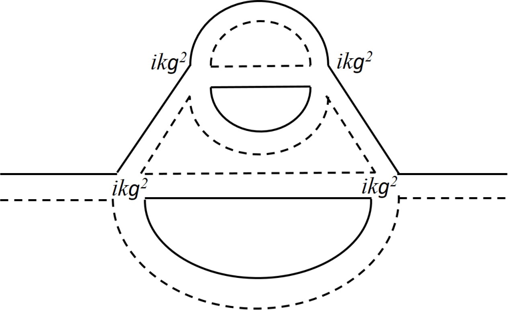
It is convenient to adopt a double-line notation for the Feynman diagrams, where a solid line represents $I=n+1,\cdots N$, and a dashed line represents $\alpha=1,\cdots n.$ We first compute the ordinary RG equation in the large-$N$ limit without the WZW term. We will calculate the beta function with $k=0$ in arbitrary dimension $d$ and insert the physical value $d=3$. In terms of the dimensionless coupling $\tilde{g}=\Lambda^{d-2}g$ and $\tilde{g}^{\prime}=\Lambda^{d-2}g^{\prime}$ ($\Lambda\sim 1/l$ is the ultraviolet momentum cut-off), the beta functions in the large-$N$ limit for the ordinary NLSM (with $k=0$) are

in our current case $d=3$. As long as $n\sim N^{A}$ with $A<1$, in the large-$N$ limit we only need to keep these terms in the beta functions. Eq. 36 has several fixed points. If we start with the physical parameter $\tilde{g}(\Lambda)=\tilde{g}^{\prime}(\Lambda)$ as the tuning parameter at the beginning of the RG flow, then increasing $\tilde{g}$ will lead to a quantum phase transition controlled by the fixed point

and the critical exponent $\nu=1$. The location of the critical point, and the critical exponent is consistent with the well-known result of the CP^N-1 model in the large$-N$ limit [26, 27].

Now let us compute the beta functions with the WZW term. Naively one would expect that the leading order contribution from the WZW term to the beta functions is the one-loop diagram Fig. 1. But because the numerator of the WZW vertex is completely antisymmetric in momenta, this diagram does not renormalize the coupling constants $g$ and $g^{\prime}$. Fig. 2 is a two-loop planar wave function renormalization diagram that renormalizes $g$ and $g^{\prime}$. This diagram leads to the following corrections to the beta functions:

In this equation $c$ is a positive number whose exact value is unimportant, because we are going to treat $k^{2}$ as a tuning parameter.

Our goal is to look for a stable fixed point which corresponds to a stable $(2+1)d$ CFT in the quantum disordered phase. The negative sign of the $k^{2}$ term in Eq. 40 suggests that this is possible. However, to make a confident conclusion, we need to choose certain adequate scaling between $k$ and $N$: $k\sim N^{B}$. If for instance $0<B\leq 3/2$, then the $k^{2}$ terms in Eq. 40 indeed lead to a new stable fixed point in the quantum disordered phase at $\tilde{g}_{\ast}\sim k^{-2/3}\geq 1/N$ and $\tilde{g}^{\prime}_{\ast}=0$. But around this “new fixed point”, infinite number of higher loop diagrams would become nonperturbative. For example, let us examine the four-loop WZW contribution, which is shown in Fig. 3. This diagram has seven internal propagators, four WZW vertices, two closed solid loops, and two closed dashed loops. Therefore this diagram contributes a term $\sim g^{9}k^{4}n^{2}N^{2}$ to the beta function. Then when $B\leq 3/2$, this four-loop diagram (and infinite number of higher loop diagrams) also contributes at least at the same order as the $k^{2}$ terms in Eq. 40, around the “new fixed point” $\tilde{g}_{\ast}\sim k^{-2/3}$.

But on the other hand, if $B>3/2$, then the $k^{2}$ term in Eq. 40 would be too large and make the entire RG equations flow to $\tilde{g}=\tilde{g}^{\prime}=0$. We stress that these difficulties only occur with the presence of the WZW term. Without the WZW term, this theory does have a simple large-$N$ limit.

In order to find a controlled calculation and to identify the stable fixed point in the quantum disordered phase with confidence, we need to find another small parameter to expand with. As we mentioned before we cannot rely on the ordinary $2+\epsilon$ expansion in our case. In this section we propose a possible solution to this difficulty in our current context by introducing a different $\epsilon-$generalization of our model.

We first test our approach with $n=1$ ($\mathcal{M}=\mathrm{CP}^{N-1}$). We generalize the original action Eq. 17 as following:

Here the notation $|\bar{\partial}|$ is most manifest in the momentum space: $A^{\dagger}|\bar{\partial}|B$ in the momentum space corresponds to $A^{\dagger}(\vec{p})|\frac{1}{2}(\vec{p}+\vec{q})|B(\vec{q})$. This nonanalytic generalization can be made systematically to all higher order expansion of the Lagrangian: a singular momentum dependence $|\bar{\partial}|^{\frac{\epsilon-1}{2}}$ is inserted in $\phi^{\dagger}\cdot\partial_{\mu}\phi$ and $\phi\cdot\partial_{\mu}\phi^{\dagger}$, and $|\bar{\partial}|^{\epsilon-1}$ is inserted in $\phi^{\dagger}\cdot\phi$. At least in the large$-N$ limit, it can be shown that all the relevant renormalizations to this Lagrangian can still be absorbed into the RG flow of $g$ and $g^{\prime}$.

The nonanalytic generalization of a local field theory dated back to studies on spin systems with long range interactions [28], and the study of the Gross-Neveu model [29]. Later a generalization of the regular $p^{2}$ kinetic term to $|p|^{1+\epsilon}$ was used as a controlled calculation method for $2d$ Fermi surface coupled with a bosonic field [30, 31, 32], which without the nonanalytic generalization also suffers from the infinite diagram difficulty in the large-$N$ limit [33]. The advantage of the nonanalytic generalization is that, now the scaling dimension of $g$ and $g^{\prime}$ at weak interacting limit becomes $-\epsilon$, and we can treat $\epsilon$ as another small parameter to organize all the Feynman diagrams.

The WZW term is now generalized to

When $n=1$ there is no higher order terms in the WZW term, which significantly simplifies the analysis. When $\epsilon=1$ this action returns to its original form Eq. 17.

This generalization keeps many of the basic properties of the original WZW term:

1) this term Eq. 52 is always purely imaginary;

2) like the WZW term, the parameter $k$ is always marginal for arbitrary $\epsilon$, which is guaranteed by the nonanalytic momentum dependence inserted in the generalized WZW term;

3) the two $\phi$ ($\phi^{\dagger}$) fields in Eq. 52 are equivalent to each other.

With large-$N$ and leading order in $\epsilon$, the RG equations of $\tilde{g}$ and $\tilde{g}^{\prime}$ read (here we redefine $\tilde{g}=\Lambda^{\epsilon}g$ and $\tilde{g}^{\prime}=\Lambda^{\epsilon}g^{\prime}$ to make them dimensionless)

$\beta(\tilde{g})_{0}^{(\epsilon)}$ and $\beta(\tilde{g}^{\prime})_{0}^{(\epsilon)}$ are simply $\beta(\tilde{g})_{0}$ and $\beta(\tilde{g}^{\prime})_{0}$ with the first term replaced by $-\epsilon\tilde{g}$ and $-\epsilon\tilde{g}^{\prime}$. The wave function renormalization Fig. 2 is the only diagram that contributes to the last terms in Eq. 53 in the large$-N$ limit. Vertex corrections in Fig. 4 will not contribute here because under RG flow it generates an $\phi^{4}$ term with analytic momentum dependence, which is less relevant compared with the terms in Eq. 51. The absence of vertex corrections here is similar to the absence of boson field wave function renormalization discussed in Ref. 31, basically because a nonanalytic momentum dependence cannot be generated by integrating out high momentum degrees of freedom in RG. This absence of vertex correction to terms with nonanalytic momentum dependence was also discussed in Ref. 35, 34.

Now we need to take $k^{2}\sim(N/\epsilon)^{3}$ to keep all the terms in these equations at the same order, and we expect that the fixed points of these beta functions will be around $\tilde{g}\sim\epsilon/N$. With small enough $\epsilon$, the terms we keep in Eq. 53 will be dominant compared with all higher loop diagrams.

The value of constant $c$ is computed at $\epsilon=0$: with large-$N$, large-$k$ and $\epsilon=0$, the wave function renormalization in Fig. 2 will lead to the following correction to the coupling constant $g$:

where $\Lambda$ and $\Lambda^{\prime}$ are the ultraviolet cut-off and rescaled cut-off. Thus $c=1/(3\pi^{2})$. The value of $c$ evaluated at $\epsilon=0$ depends on the exact form of the $\epsilon$ generalization of the WZW term.

We take $k^{2}=G^{3}(N/\epsilon)^{3}$ with small coefficient $G$. Eq. 53 generates several fixed points. If we start with the physical parameters $\tilde{g}(\Lambda)=\tilde{g}^{\prime}(\Lambda)$ at the beginning of the RG, the flow of the parameters is controlled by two of these fixed points. The first fixed point is the order-disorder quantum phase transition located at

and the critical exponent $1/\nu$ is

If we extrapolate $\epsilon$ to $1$, $\nu$ will be greater than 1, which can already be expected from the negative sign of the $k^{2}$ term in the beta functions. This is qualitatively different from the critical exponent without the WZW term. For instance it is well-known that the $(2+1)d$ CP^N-1 model has $\nu<1$ with $1/N$ correction taken into account [27].

Most importantly, there is a stable fixed point in the quantum disordered phase:

We need $G$ small enough to guarantee that the coupling constant in Eq. 63 is larger than the one in Eq. 61, $i.e.$ the system is in a quantum disordered phase. In the vicinity of this new stable fixed points, the beta functions give the scaling dimension of two irrelevant perturbations:

Both scaling dimensions are negative with small enough $G$. The RG flow diagram for the RG equations with parameters $\epsilon=0.05$ $N=10$, $ck^{2}n\sim 340$ is plotted in Fig. 5.

In order to carry out the calculation for $n>1$, we need to include higher order terms in the expansion of the WZW term. We also need to generalize the $\mathcal{O}(\phi^{6})$ order in the WZW term to a nonanalytic form. There are certainly more than one possible $\epsilon-$generations, as an example, we choose the following form for the $\phi^{6}$ term in the momentum space:

This generalization still keeps the basic properties of the WZW term that we need to carry out the calculations, and when $\epsilon=1$ it returns to the original form of the WZW term. This $\phi^{6}$ term so designed only generates irrelevant terms in the large$-N$ limit and leading order $\epsilon$ expansion. For example, Fig. 6 is a leading order diagram in terms of large$-N$ and $\epsilon-$expansion counting, but it only generates an irrelevant analytic term to the Lagrangian.

In this work we did our best to search for a controlled study of stable interacting conformal field theories at the boundary of $(3+1)d$ SPT states. We performed calculation in the large$-N$ limit and leading order $\epsilon-$expansion, and the desired stable fixed point is indeed found in the quantum disordered phase. But we have not proved that higher order expansions will not generate more relevant terms in the Lagrangian.

Besides exploring the exotic boundary states of $(3+1)d$ bosonic SPT phases, another motivation of this work was the “hierarchy problem” in high energy physics: why the Higgs boson is so much lighter than the Planck mass? Compared with the Planck mass, the Higgs boson, which is a space-time scalar, is almost massless. Gauge bosons, which can emerge very naturally in condensed matter systems [36, 37, 38], indeed have zero mass. But a space-time scalar boson, unless it is a Goldstone mode, usually acquires a mass that is comparable with the ultraviolet cut-off without fine-tuning to a critical point. At least this is the case for space-time dimensions higher than $(1+1)d$ (in $(1+1)d$ space-time scalar bosons can easily form a conformal field theory). Indeed, the little Higgs theory hypothesizes that the Higgs boson itself is a pseudo Goldstone boson [39, 40, 41, 42], which explains its small mass. The result of our current work suggests another possible route to address the hierarchy problem: the Higgs boson could be rendered massless due to a topological WZW term, even if the system is in a quantum disordered phase, $i.e.$ there is no (pseudo) spontaneous symmetry breaking. But, in order to show this explicitly, one needs to first embed the Higgs boson into a larger target manifold $\mathcal{M}$ which permits a WZW term, and perform a controlled RG calculation in $(3+1)d$ ³³ 3 $\pi_{5}[SU(N)]=\mathbb{Z}$ for $N>2$, thus a matrix model whose target manifold is $SU(N)$ could have a WZW term in $(3+1)d$. But $SU(N)$ matrix model does not have a controlled large$-N$ limit even without the WZW term.. We will leave this direction to future study.

At the purely technical level, although the WZW term can be formally rewritten as a Chern-Simons term, we cannot treat the gauge field $a_{\mu}$ (Eq. 13) in the path integral as if it were an independent degree of freedom with a Chern-Simons term. For example, when $N=2n=2$, the topological term becomes the quantized Hopf term if written in terms of $\varphi^{i}$, while the Chern-Simons action of a U(1) gauge field is in general not quantized. The WZW term can only be interpreted as the Chern-Simons term if Eq. 13 holds rigorously. However, if a Chern-Simons term of $a_{\mu}$ is already included in the action, the equation of motion of the gauge field is no longer given by Eq. 13. In the standard path integral formalism of the CP^N-1 model, the gauge field $a_{\mu}$ is introduced as an auxiliary field through the Hubbard-Stratonovich transformation. Thus one should introduce one more vector field $b_{\mu}$ through the Hubbard-Stratonovich transformation on the WZW term: $\sim ik\varepsilon\varphi^{\dagger}\cdot\partial\varphi\partial b+ik\varepsilon b\partial b$ (indices and unimportant factors are omitted in this equation). Integrating out $b_{\mu}$ will regenerate the WZW term, for the simplest case $n=1$. For $n>1$ this method gets more complicated.

Bi, Rasmussen and Xu are supported by the David and Lucile Packard Foundation and NSF Grant No. DMR-1151208. BenTov is supported by the Simons Foundation Agency with award number: 376205. The authors thank Leon Balents and Andreas Ludwig for helpful discussions.

References

- [1] X. Chen, Z.-C. Gu, Z.-X. Liu, and X.-G. Wen, Phys. Rev. B 87, 155114 (2013).
- [2] X. Chen, Z.-C. Gu, Z.-X. Liu, and X.-G. Wen, Science 338, 1604 (2012).
- [3] Y.-M. Lu and A. Vishwanath, Phys. Rev. B 86, 125119 (2012).
- [4] L. Fidkowski, X. Chen, and A. Vishwanath, Phys. Rev. X 3, 041016 (2013).
- [5] X. Chen, L. Fidkowski, and A. Vishwanath, Phys. Rev. B 89, 165132 (2014).
- [6] P. Bonderson, C. Nayak, and X.-L. Qi, J. Stat. Mech. p. P09016 (2013).
- [7] M. A. Metlitski, C. L. Kane, and M. P. A. Fisher, arXiv:1306.3286 (2013).
- [8] C. Wang, A. C. Potter, and T. Senthil, Phys. Rev. B 88, 115137 (2013).
- [9] A. Vishwanath and T. Senthil, Phys. Rev. X 3, 011016 (2013).
- [10] Z. Bi, A. Rasmussen, and C. Xu, Phys. Rev. B 91, 134404 (2015).
- [11] C. Xu and T. Senthil, Phys. Rev. B 87, 174412 (2013).
- [12] C. Xu, Phys. Rev. B 87, 144421 (2013).
- [13] E. Witten, Commun. Math. Phys. 92, 455 (1984).
- [14] V. G. Knizhnik and A. B. Zamolodchikov, Nucl. Phys. B 247, 83 (1984).
- [15] E.-G. Moon, Phys. Rev. B 85, 245123 (2012).
- [16] K. Slagle, Y.-Z. You, and C. Xu, Phys. Rev. B 91, 115121 (2015).
- [17] Y.-Y. He, H.-Q. Wu, Y.-Z. You, C. Xu, Z. Y. Meng, and Z.-Y. Lu, ArXiv e-prints (2015), eprint 1508.06389.
- [18] T. Senthil, A. Vishwanath, L. Balents, S. Sachdev, and M. P. A. Fisher, Science 303, 1490 (2004a).
- [19] T. Senthil, L. Balents, S. Sachdev, A. Vishwanath, and M. P. A. Fisher, Phys. Rev. B 70, 144407 (2004b).
- [20] T. Senthil and M. P. A. Fisher, Phys. Rev. B 74, 064405 (2005).
- [21] A. G. Abanov, Phys. Lett. B 321, 492 (2000).
- [22] C. Wang and T. Senthil, Phys. Rev. B 89, 195124 (2014).
- [23] S. Hikami, Prog. Theor. Phys. 64, 1466 (1980).
- [24] E. Brezin, S. Hikami, and J. Zinn-Justin, Nucl. Phys. B 165, 528 (1980).
- [25] X.-L. Qi, T. L. Hughes, and S.-C. Zhang, Phys. Rev. B 78, 195424 (2008).
- [26] B. I. Halperin, T. C. Lubensky, and S. keng Ma, Phys. Rev. Lett. 32, 292 (1974).
- [27] R. K. Kaul and S. Sachdev, Phys. Rev. B 77, 155105 (2008).
- [28] M. E. Fisher, S. keng Ma, and B. G. Nickel, Phys. Rev. Lett. 29, 917 (1972).
- [29] K. G. Dski and A. Kupianen, Nucl. Phys. B 262, 33 (1985).
- [30] D. F. Mross, J. McGreevy, H. Liu, and T. Senthil, Phys. Rev. B 82, 045121 (2010).
- [31] C. Nayak and F. Wilczek, Nucl. Phys. B 417, 359 (1994a).
- [32] C. Nayak and F. Wilczek, Nucl. Phys. B 430, 534 (1994b).
- [33] S.-S. Lee, Phys. Rev. B 80, 165102 (2009).
- [34] C. Xu, M. Mueller, and S. Sachdev, Phys. Rev. B 78, 020501(R) (2008).
- [35] E. Frey and L. Balents, Phys. Rev. B 55, 1050 (1997).
- [36] X.-G. Wen, Phys. Rev. B 68, 115413 (2003).
- [37] R. Moessner and S. L. Sondhi, Phys. Rev. B 68, 184512 (2003).
- [38] M. Hermele, M. P. A. Fisher, and L. Balents, Phys. Rev. B 69, 064404 (2004).
- [39] N. Arkani-Hamed, A. G. Cohen, and H. Georgi, Phys. Rev. B 513, 232 (2001).
- [40] N. Arkani-Hamed, A. G. Cohen, E. Katz, A. E. Nelson, T. Gregoire, and J. G. Wacker, JHEP 0208, 019 (2002a).
- [41] N. Arkani-Hamed, A. G. Cohen, E. Katz, and A. E. Nelson, JHEP 0207, 034 (2002b).
- [42] D. E. Kaplan and M. Schmaltz, JHEP 0310, 039 (2003).