跳到论文正文
W Papers独立论文阅读器 arXiv:1605.05266 论文正文 计算阅读时间 · 0%
引用这篇论文根据当前论文元数据生成,正式投稿前建议核对。


License: arXiv.org perpetual non-exclusive license
arXiv:1605.05266v1 [math.AP] 17 May 2016

Remarks on functions with bounded Laplacian

Tarek M. Elgindi Address: Department of Mathematics, Princeton University, Princeton, NJ 08544 Email address: tme2@.princeton.edu
Date: August 24, 2026
Abstract.

Δ​ψ:=∂2ψ∂x12+∂2ψ∂x22\Delta\psi:=\frac{\partial^{2}\psi}{\partial x_{1}^{2}}+\frac{\partial^{2}\psi}{\partial x_{2}^{2}} being locally bounded does not imply that D2​ψD^{2}\psi is locally bounded. However, we prove that if ψ\psi is invariant under rotation by 2​πm\frac{2\pi}{m}, for some m≥3m\geq 3, and Δ​ψ\Delta\psi is locally bounded, then

supx∈B1​(0)|∇ψ​(x)||x|<∞.\sup_{x\in B_{1}(0)}\frac{|\nabla\psi(x)|}{|x|}<\infty.

This is sharp in that there are examples of functions ψ\psi for which Δ​ψ\Delta\psi is locally bounded, which are invariant under rotation by π\pi with |ψ⁡(x)−ψ⁡(0)|≈|x|2​|log⁡|x|||\psi(x)-\psi(0)|\approx|x|^{2}|\log|x|| as |x|→0|x|\rightarrow 0. This bound and its generalizations could be of use in different contexts, particularly for questions about singularity formation in evolution equations. We came upon it while studying certain singular solutions of the incompressible Euler equations in two dimensions (see [5]). One other application is to prove boundedness of D2​ψD^{2}\psi when Δ​ψ\Delta\psi is the characteristic function of a set with self-intersection points (see Section 5). In fact, if Δ​ψ=χA\Delta\psi=\chi_{A} and AA is the union of sectors emanating from a single point, one can give necessary and sufficient conditions on AA for D2​ψD^{2}\psi to be locally bounded (see Section 6).

1. Introduction

The problem of inverting the Laplacian is one of the fundamental classical problems in mathematical analysis. The basic existence question is: when can we recover a function of nn variables, ψ⁡(x1,…,xn),\psi(x_{1},...,x_{n}), from its Laplacian, Δ​ψ:=∑i=1n∂2ψ∂xi2\Delta\psi:=\sum_{i=1}^{n}\frac{\partial^{2}\psi}{\partial{x_{i}}^{2}}? The related regularity question is: given that Δ​ψ\Delta\psi belongs to a certain function space, is it true that D2​ψD^{2}\psi also belongs to that same function space? There are numerous situations when both the existence and regularity question can be answered affirmatively. For the regularity question, when the function space is LpL^{p} for 1<p<∞1<p<\infty or CαC^{\alpha}, 0<α<10<\alpha<1, the answer is generally yes. One notable “borderline” case which is troublesome for the regularity question is when the function space is L∞L^{\infty}.

More formally, given f∈L∞f\in L^{\infty} with compact support, consider the problem of finding ψ\psi such that

Δ​ψ=f,in​ℝ2.\Delta\psi=f,\,\,\,\text{in}\,\,\,\mathbb{R}^{2}.

Classical results give us that any ψ\psi solving this equation must belong to Wl​o​c2,pW^{2,p}_{loc} for every p<∞p<\infty (see for example the book of Gilbarg and Trudinger [7]). In fact, D2​ψ∈B​M​OD^{2}\psi\in BMO, the space of functions of bounded mean-oscillation. However, D2​ψD^{2}\psi need not belong to Ll​o​c∞L^{\infty}_{loc}. In fact, D2​ψD^{2}\psi may be unbounded near jump discontinuities of ff, though only logarithmically so. This problem is very much related to the unboundedness of singular integrals on L∞.L^{\infty}. Indeed, using the Newtonian potential, we can write

ψ⁡(x)=12​π​∫log⁡|x−y|​f​(y)​𝑑y.\psi(x)=\frac{1}{2\pi}\int\log|x-y|f(y)dy.

One can then deduce properties of D2​ψD^{2}\psi from differentiating the integral in the proper way. It can then be seen that D2​ψD^{2}\psi is a matrix of singular integrals applied to f:f:

−D2​ψ=[R12​fR1​R2​fR1​R2​fR22​f]-D^{2}\psi=\begin{bmatrix}R_{1}^{2}f&R_{1}R_{2}f\\ R_{1}R_{2}f&R_{2}^{2}f\ \end{bmatrix}

where R1R_{1} and R2R_{2} are the standard Riesz transforms on ℝ2:\mathbb{R}^{2}:

Ri​(f):=P.V.​12​π​∫ℝ2xi−yi|x−y|3​f​(y)​𝑑y,R_{i}(f):=\text{P.V.}\frac{1}{2\pi}\int_{\mathbb{R}^{2}}\frac{x_{i}-y_{i}}{|x-y|^{3}}f(y)dy,

where the integral is understood in the sense of the principal value. The problem of getting L∞L^{\infty} bounds on D2​ψD^{2}\psi from L∞L^{\infty} bounds on Δ​ψ\Delta\psi then is equivalent to studying the boundedness of the Riesz transforms R12,R22,R_{1}^{2},R_{2}^{2}, and R1​R2R_{1}R_{2} on L∞L^{\infty}.

1.1. Borderline Inequalities

While it would seem that one should just avoid L∞L^{\infty} when inverting the Laplacian, many problems in the study of non-linear partial differential equations force us to work with L∞L^{\infty}. This tension has begotten many interesting so-called borderline inequalities where authors try to quantify losses incurred by working with L∞.L^{\infty}. A good example of this are the stream of Brezis-Gallouet-Wainger, Moser-Trudinger, and Bourgain-Brezis inequalities (see [2]). Though many of those inequalities deal with the lack of critical Sobolev embeddings into L∞L^{\infty}, some of them also deal with the problem of deriving estimates on D2​ψD^{2}\psi from estimates on Δ​ψ\Delta\psi. For example, Brezis and Gallouet proved that given that ψ∈C2,α​(Ω¯)\psi\in C^{2,\alpha}(\overline{\Omega}) and ψ=0\psi=0 on ∂Ω\partial\Omega for Ω\Omega a smooth and bounded domain,

|D2​ψ|L∞≤C​|Δ​ψ|L∞​log⁡(|ψ|C2,α|Δ​ψ|L∞+10)|D^{2}\psi|_{L^{\infty}}\leq C|\Delta\psi|_{L^{\infty}}\log(\frac{|\psi|_{C^{2,\alpha}}}{|\Delta\psi|_{L^{\infty}}}+10)

for some universal constant C>0.C>0.

The use of this inequality is to be able to assert that while D2​ψD^{2}\psi cannot be bounded point-wise by the maximum of |Δ​ψ||\Delta\psi| alone, one could do this with a logarithmic loss. Such inequalities play a crucial role in global well-posedness proofs in various contexts in the study of evolution equations.

1.2. Jump Discontinuities Across Smooth Curves

In certain situations, D2​ψD^{2}\psi may belong to L∞L^{\infty} even if Δ​ψ\Delta\psi has jump discontinuities. This, however, depends upon the geometry of the jump discontinuities of Δ​ψ.\Delta\psi. For example, if Δ​ψ\Delta\psi is the characteristic function of a set with smooth boundary, it can be shown that D2​ψ∈L∞.D^{2}\psi\in L^{\infty}. One does this by observing that if Δ​ψ\Delta\psi is characteristic function of a set AA with smooth boundary, then ψ\psi is smooth in the direction tangential to the boundary. Looking at the case when A=ℝ+2A=\mathbb{R}^{2}_{+}, the upper half plane, is quite revealing. In fact, an improvement on the Brezis-Gallouet inequality can actually be proven in this context [4].11 1 It must be mentioned that the Brezis-Gallouet inequality can actually be used to control D2​ψD^{2}\psi in the Besov space B∞,10B^{0}_{\infty,1} which controls any number of Riesz transforms of D2​ψD^{2}\psi in L∞L^{\infty}, whereas anisotropic regularity only allows one to control Riesz transforms of the form R1j​R2iR_{1}^{j}R_{2}^{i} with i+j∈2​ℤi+j\in 2\mathbb{Z}. This can be done by direct analysis of the Green’s function for the Laplacian as is done in [4],[3]. This cannot be done, however, when Δ​ψ\Delta\psi is the characteristic function of a set which has a corner because there are numerous examples where Δ​ψ\Delta\psi is the characteristic function of a set which is smooth away from a single corner and for which D2​ψD^{2}\psi is unbounded near the corner.

1.3. The Main Result

Up to now, we have seen two ways to propagate L∞L^{\infty} bounds on D2​ψD^{2}\psi from bounds on Δ​ψ\Delta\psi. Both cases require that Δ​ψ\Delta\psi enjoy some extra regularity (be it isotropic or anisotropic). There still remains the question: is there a way to control |D2​ψ||D^{2}\psi| just by |Δ​ψ|L∞​?|\Delta\psi|_{L^{\infty}}? In this short note, we give one case where this can, effectively, be done. In fact, we prove that if Δ​ψ\Delta\psi is invariant under rotation by 2​πm\frac{2\pi}{m} for some m≥3m\geq 3, then,

|∇ψ​(x)||x|≤C\frac{|\nabla\psi(x)|}{|x|}\leq C

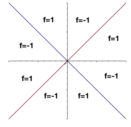
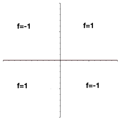
as x→0x\rightarrow 0 without any further regularity assumptions on ψ\psi.22 2 Clearly, this can be relaxed to the case where Δ​ψ\Delta\psi is invariant under rotation by 2​πm\frac{2\pi}{m} only in a neighborhood of 00. The following two examples of piece-wise constant functions ff illustrate the importance of the symmetry assumption:
Refer to caption
Refer to caption
Figure 1. If Δ​ψ=f\Delta\psi=f with ff the piecewise constant function on the right, then D2​ψ∈L∞D^{2}\psi\in L^{\infty}. However, if Δ​ψ=f\Delta\psi=f with ff the piecewise constant function on the left, then |∇ψ|≈|x|​|log⁡|x|||\nabla\psi|\approx|x||\log|x|| near |x|=0|x|=0.

These two examples illustrate the following simple fact: corner-like discontinuities in Δ​ψ\Delta\psi may lead to D2​ψD^{2}\psi being unbounded, but only in certain geometric configurations. In other situations, where more symmetries are present near the corner, D2​ψD^{2}\psi will remain bounded.

1.4. The 2d Incompressible Euler Equations

We now discuss one particular example of a non-linear evolution equation where information about inverting the Laplacian on L∞L^{\infty} is very important. Recall the 2d incompressible Euler equations in a smooth bounded domain Ω\Omega:

(1.1) ∂tω+u⋅∇ω=0,\partial_{t}\omega+u\cdot\nabla\omega=0,
(1.2) u=∇⟂ψ,u=\nabla^{\perp}\psi,

where ψ\psi is the unique solution of:

Δ​ψ=ω​in​Ω,\Delta\psi=\omega\,\,\,\text{in}\,\,\,\Omega,
ψ=0​on​∂Ω.\psi=0\,\,\,\text{on}\,\,\,\partial\Omega.

It is clear that smooth enough solutions of (1.1)-(1.2) satisfy:

dd​t​|ω|Lp​(t)=0,\frac{d}{dt}|\omega|_{L^{p}}(t)=0,

for all t∈ℝt\in\mathbb{R} and all 1≤p≤∞1\leq p\leq\infty. In particular, smooth solutions satisfy an a-priori L∞L^{\infty} estimate. The Yudovich theory ([12]) allows us to construct unique global solutions to (1.1)-(1.2) for given ω0∈L∞\omega_{0}\in L^{\infty}. This is due to the fact that an L∞L^{\infty} estimate on ω\omega automatically implies a quasi-Lipschitz estimate on uu which, in turn, allows us to control the Lagrangian flow-map associated to u.u. This is all discussed in detail in [12] so we do not repeat it here. The L∞L^{\infty} estimate on ω\omega also allows us to construct a unique global smooth solution to (1.1)-(1.2) from smooth initial data. However, due to the fact that the L∞L^{\infty} estimate on ω\omega only implies a quasi-Lipschitz bound on uu (or using the borderline inequality of Subsection 1.1), one can prove that smooth solutions of (1.1)-(1.2) satisfy a double exponential type bound:

|∇ω​(t)|L∞≤|ω0|L∞​(|∇ω0|L∞|ω0|L∞)exp⁡(C​|ω0|L∞​t),|\nabla\omega(t)|_{L^{\infty}}\leq|\omega_{0}|_{L^{\infty}}\Big(\frac{|\nabla\omega_{0}|_{L^{\infty}}}{|\omega_{0}|_{L^{\infty}}}\Big)^{\exp(C|\omega_{0}|_{L^{\infty}}t)},

for some universal constant C>0.C>0.

The reason that this double exponential growth might be possible is precisely because a bound on ω\omega in L∞L^{\infty} does not imply a W2,∞W^{2,\infty} bound on Δ−1​ω\Delta^{-1}\omega. Hence having a good understanding on when L∞L^{\infty} bounds on ω\omega imply a W2,∞W^{2,\infty} bound on Δ−1​ω\Delta^{-1}\omega is very important to understand the mechanisms which lead to double exponential growth of ∇ω\nabla\omega. Improving on this double-exponential estimate in general seems to be a great challenge. In fact, when the 2d Euler equations are studied on smooth bounded domains which are symmetric with respect to some line in ℝ2\mathbb{R}^{2}, the double exponential bound is known to be optimal in full generality [9],[10], though the growth is only known to be possible on the boundary. In fact, the constructions in [9] and [10] rely on proving that for certain initial data (satisfying a suitable symmetry condition) t→∞t\rightarrow\infty,

sup|x|≤c|∇ψ​(x)||x|≥eC​t,\sup_{|x|\leq c}\frac{|\nabla\psi(x)|}{|x|}\geq e^{Ct},

which is precluded under our symmetry condition. It is possible that the idea of this paper could be used to preclude double-exponential growth of ∇ω\nabla\omega away from the boundary. This seems somewhat related to the work of Itoh, Miura, and Yoneda [11].

1.5. Organization of the Paper

In the second section of this note, we discuss some important examples which will help to build intuition about the sorts of issues one faces when inverting the Laplacian on L∞.L^{\infty}. In the third section we state and prove the main lemma. In the fourth section we discuss various direct extensions. In Sections 5 and 6 we study the problem of solving

Δ​ψ=χA\Delta\psi=\chi_{A}

when AA is a bounded Lipschitz domain.

2. Counterexamples

In this section we discuss several types of examples which illustrate the difficulty of inverting the Laplacian on L∞L^{\infty}.

2.1. Counterexample 1: Using harmonic polynomials

Let PP be a harmonic polynomial on ℝ2\mathbb{R}^{2} which is homogeneous of degree 2. In fact, there are only two possibilities for PP (up to scaling): P⁡(x1,x2)=x1​x2P(x_{1},x_{2})=x_{1}x_{2} or P⁡(x1,x2)=x12−x22P(x_{1},x_{2})=x_{1}^{2}-x_{2}^{2}. Note that neither of these are invariant under rotation by π2\frac{\pi}{2} (they are, in fact, “odd”). Let ϕ\phi be a smooth function which is identically 1 in B1​(0)B_{1}(0) and identically 00 outside of B2​(0)B_{2}(0). Now define

ψP=P⁡(x1,x2)​log⁡|x12+x22|​ϕ​(x1,x2).\psi_{P}=P(x_{1},x_{2})\log|x_{1}^{2}+x_{2}^{2}|\phi(x_{1},x_{2}).

Observe that ψP\psi_{P} is smooth away from (0,0)(0,0) and that on B1​(0)B_{1}(0), ΔψP=∇P⋅4​x|x|2.\Delta\psi_{P}=\nabla P\cdot\frac{4x}{|x|^{2}}. Since PP is homogenous of degree 2, Δ​ψp∈L∞\Delta\psi_{p}\in L^{\infty}. On the other hand, clearly D2​ψP∉L∞D^{2}\psi_{P}\not\in L^{\infty} and

|∇ψP|≈−|x|​log⁡|x|,|\nabla\psi_{P}|\approx-|x|\log|x|,

near |x|=0|x|=0.

We note here that this example can be found in the book of Han and Lin [LinHan].

2.2. Counterexample 2: Using Fourier series

Define

ψ⁡(x,y)=∑n,m=1∞sin⁡(n​x)​sin⁡(m​y)n​m​(n2+m2).\psi(x,y)=\sum_{n,m=1}^{\infty}\frac{\sin(nx)\sin(my)}{nm(n^{2}+m^{2})}.

Notice that

Δ​ψ=∑m,n=1∞sin⁡(n​x)​sin⁡(m​y)n​m=s​g​n​(x)​s​g​n​(y)\Delta\psi=\sum_{m,n=1}^{\infty}\frac{\sin(nx)\sin(my)}{nm}=sgn(x)sgn(y)

on [−π,π]2[-\pi,\pi]^{2}. Hence, Δ​ψ∈L∞\Delta\psi\in L^{\infty}. However,

∂x​yψ=∑n,m=1∞cos⁡(n​x)​cos⁡(m​y)n2+m2.\partial_{xy}\psi=\sum_{n,m=1}^{\infty}\frac{\cos(nx)\cos(my)}{n^{2}+m^{2}}.

It can be easily checked that ∂x​yψ\partial_{xy}\psi is like |log⁡|x|||\log|x|| near |x|=0|x|=0. Notice that ψ\psi is not invariant under rotation by 2​πm\frac{2\pi}{m} for any m≥3m\geq 3.

2.3. Counterexample 3: The characteristic function of a set with a corner

Consider, for example,

Δ​ψ=χ[0,1]2.\Delta\psi=\chi_{[0,1]^{2}}.

We will show that

|∇ψ−∇ψ​(0)|≈|x|​|log⁡|x||.|\nabla\psi-\nabla\psi(0)|\approx|x||\log|x||.

Using the Green’s function representation for ψ\psi, we get:

∂x1ψ⁡(x)=∫ℝ2x1−y1|x−y|2​Δ​ψ​(y)​𝑑y=∫[0,1]2x1−y1|x−y|2​𝑑y\partial_{x_{1}}\psi(x)=\int_{\mathbb{R}^{2}}\frac{x_{1}-y_{1}}{|x-y|^{2}}\Delta\psi(y)dy=\int_{[0,1]^{2}}\frac{x_{1}-y_{1}}{|x-y|^{2}}dy
=∫01∫01x1−y1(x1−y1)2+(x2−y1)2​𝑑y=∫0112​log⁡((x2−y2)2+(x1)2(x2−y2)2+(1−x1)2)​d​y2.=\int_{0}^{1}\int_{0}^{1}\frac{x_{1}-y_{1}}{(x_{1}-y_{1})^{2}+(x_{2}-y_{1})^{2}}dy=\int_{0}^{1}\frac{1}{2}\log(\frac{(x_{2}-y_{2})^{2}+(x_{1})^{2}}{(x_{2}-y_{2})^{2}+(1-x_{1})^{2}})dy_{2}.

Hence, ∂x1u⁡(0,0)=∫01log⁡y22y22+1​d​y2.\partial_{x_{1}}u(0,0)=\int_{0}^{1}\log\frac{y_{2}^{2}}{y_{2}^{2}+1}dy_{2}. Moreover, ∂x1u⁡(0,x2)=∫01log⁡(x2−y2)2(x2−y2)2+1​d​y2.\partial_{x_{1}}u(0,x_{2})=\int_{0}^{1}\log\frac{(x_{2}-y_{2})^{2}}{(x_{2}-y_{2})^{2}+1}dy_{2}. Therefore,

∂x1u⁡(0,x2)−∂x1u⁡(0,0)=∫01log⁡(x2−y2)2y22+∫01log⁡y22+1(x2−y2)2+1​d​y2\partial_{x_{1}}u(0,x_{2})-\partial_{x_{1}}u(0,0)=\int_{0}^{1}\log\frac{(x_{2}-y_{2})^{2}}{y_{2}^{2}}+\int_{0}^{1}\log\frac{y_{2}^{2}+1}{(x_{2}-y_{2})^{2}+1}dy_{2}
=∫01log⁡(x2−y2)2y22​d​y2+O⁡(x2).=\int_{0}^{1}\log\frac{(x_{2}-y_{2})^{2}}{y_{2}^{2}}dy_{2}+O(x_{2}).

Now,

∫01log⁡(x2−y2)2y22​d​y2=∫−x11−x2log⁡y22​d​y2−∫01log⁡y22​d​y2=∫0x2log⁡y22​d​y2−∫1−x21log⁡y22​d​y2\int_{0}^{1}\log\frac{(x_{2}-y_{2})^{2}}{y_{2}^{2}}dy_{2}=\int_{-x_{1}}^{1-x_{2}}\log{y_{2}^{2}}dy_{2}-\int_{0}^{1}\log{y_{2}^{2}}dy_{2}=\int_{0}^{x_{2}}\log y_{2}^{2}dy_{2}-\int_{1-x_{2}}^{1}\log y_{2}^{2}dy_{2}
=x2​log⁡|x22|+O⁡(x2).=x_{2}\log|x_{2}^{2}|+O(x_{2}).

In fact, this could have been done for the case where Δ​ψ=χ[0,1]2∪[0,−1]2,\Delta\psi=\chi_{[0,1]^{2}\cup[0,-1]^{2}}, which gives the unboundedness of D2​ψD^{2}\psi in the left figure of Figure 1.

We note here that this example can be found in the paper of Bahouri and Chemin [1].

2.4. The One-dimensional Case

We also mention here a short estimate in one dimension which illustrates the use of symmetry conditions.

Lemma 2.1.

Let ϕ:ℝ→ℝ\phi:\mathbb{R}\rightarrow\mathbb{R} be such that ϕ′∈B​M​O​([−1,1]).\phi^{\prime}\in BMO([-1,1]). Assume that ϕ\phi is even. Then,

|ϕ⁡(x)−ϕ⁡(0)||x|≤|ϕ′|B​M​O​([−1,1]).\frac{|\phi(x)-\phi(0)|}{|x|}\leq|\phi^{\prime}|_{BMO([-1,1])}.
Lemma 2.2.

Let Φ∈B​M​O​([−1,1])∩C1​([−1,1]−{0})\Phi\in BMO([-1,1])\cap C^{1}([-1,1]-\{0\}) be an odd function of one variable. Assume that

|Φ′​(x)|≤C|x||\Phi^{\prime}(x)|\leq\frac{C}{|x|}

for |x|>0|x|>0. Then, Φ∈L∞​([−1,1])\Phi\in L^{\infty}([-1,1]) and

|Φ|L∞≤2​|Φ|B​M​O+|​x​Φ′​(x)|L∞|\Phi|_{L^{\infty}}\leq 2|\Phi|_{BMO}+|x\Phi^{\prime}(x)|_{L^{\infty}}
Remark 2.3.

Clearly the oddness assumption is essential for both lemmas since log⁡|x|∈B​M​O​([−1,1])\log|x|\in BMO([-1,1]) and dd​x​log⁡|x|=1x.\frac{d}{dx}\log|x|=\frac{1}{x}. These results should be compared with the higher dimensional case in Lemma 4.4.

Before giving the proof, we mention a corollary of these lemmas which is a “local” Fefferman-Stein decomposition.

Corollary 2.4.

Let Φ∈B​M​O​([−1,1])∩C1​([−1,1]−{0})\Phi\in BMO([-1,1])\cap C^{1}([-1,1]-\{0\}). Assume that

|Φ′​(x)|≤C|x|.|\Phi^{\prime}(x)|\leq\frac{C}{|x|}.

Then, there exist Φ1,Φ2∈L∞​([−1,1])\Phi_{1},\Phi_{2}\in L^{\infty}([-1,1]) such that

Φ=Φ1+H⁡(Φ2),\Phi=\Phi_{1}+H(\Phi_{2}),

where HH is the Hilbert transform.

Of course this corollary is implied by the Fefferman-Stein decomposition; however, the proof of this corollary via the preceeding lemmas is much more elementary and proceeds simply by decomposing Φ\Phi into its odd and even parts and then noticing that the Hilbert transform is an isometry and maps odd functions to even functions.

Proof of Lemma 2.2.

The first lemma is by definition of the BMO norm and using that ϕ′\phi^{\prime} is odd. The second lemma can be seen as follows: Note that

1δ​∫0δ|Φ⁡(t)|​𝑑t≤|Φ|B​M​O\frac{1}{\delta}\int_{0}^{\delta}|\Phi(t)|dt\leq|\Phi|_{BMO}

for all δ>0\delta>0 since Φ\Phi is odd and using the definition of BMO. Let ϵ>0\epsilon>0. We have that

12​ϵ​∫02​ϵ|Φ⁡(x)|​𝑑x≤|Φ|B​M​O,\frac{1}{2\epsilon}\int_{0}^{2\epsilon}|\Phi(x)|dx\leq|\Phi|_{BMO},

so

1ϵ​∫ϵ2​ϵ|Φ⁡(x)|​𝑑x≤2​|Φ|B​M​O.\frac{1}{\epsilon}\int_{\epsilon}^{2\epsilon}|\Phi(x)|dx\leq 2|\Phi|_{BMO}.

But

|Φ⁡(x)−Φ⁡(ϵ)|≤Cϵ​|x−ϵ|,|\Phi(x)-\Phi(\epsilon)|\leq\frac{C}{\epsilon}|x-\epsilon|,

for all x>ϵx>\epsilon which implies that

1ϵ​∫ϵ2​ϵ|Φ⁡(x)|≥|Φ⁡(ϵ)|−C.\frac{1}{\epsilon}\int_{\epsilon}^{2\epsilon}|\Phi(x)|\geq|\Phi(\epsilon)|-C.

In particular,

|Φ⁡(ϵ)|≤2​|Φ|B​M​O+C.|\Phi(\epsilon)|\leq 2|\Phi|_{BMO}+C.

∎

3. The Lemma and its Proof

In this section we give the statement of the main lemma and its proof.

Lemma 3.1.

Let g∈L∞​(ℝ2)g\in L^{\infty}(\mathbb{R}^{2}). Assume that for all x∈ℝ2x\in\mathbb{R}^{2},

g⁡(x)=g⁡(x⟂).g(x)=g(x^{\perp}).

Let ψ∈Ll​o​c∞​(ℝ2)\psi\in L^{\infty}_{loc}(\mathbb{R}^{2}) solve

Δ​ψ=g​in​ℝ2.\Delta\psi=g\,\,\,\text{in}\,\,\,\mathbb{R}^{2}.

Then,

supx∈B1​(0)|∇ψ​(x)||x|<∞.\sup_{x\in B_{1}(0)}\frac{|\nabla\psi(x)|}{|x|}<\infty.
Corollary 3.2.

Assume that g∈L∞​(B1​(0))g\in L^{\infty}(B_{1}(0)). Assume that for all x∈B1​(0)x\in B_{1}(0), g⁡(x)=g⁡(x⟂)g(x)=g(x^{\perp}). Let ψ\psi be the unique solution of

Δ​ψ​(x)=g⁡(x),|x|<1\Delta\psi(x)=g(x),\,\,\,|x|<1
ψ⁡(x)=0,|x|=1.\psi(x)=0,\,\,\,|x|=1.

Then,

supx∈B1​(0)|∇ψ​(x)||x|≤C​|g|L∞,\sup_{x\in B_{1}(0)}\frac{|\nabla\psi(x)|}{|x|}\leq C|g|_{L^{\infty}},

for some universal constant C>0C>0.

Remark 3.3.

We have proven the lemma here in full detail for the case when gg enjoys four-fold symmetry. The general case of n−n- fold symmetry for n≥3n\geq 3 is handled in Section 4. Note that it need not be assumed that gg satisfies the symmetry condition in all of ℝ2\mathbb{R}^{2}, just in a neighborhood of the origin. This says that if gg is symmetric in a neighborhood of any of its jump discontinuities, the corresponding ψ\psi will satisfy the bounds in the lemma.

Remark 3.4.

The proof we give is based on the Green’s function for the Laplacian. It is possible that other proofs could be given that might give some insight into how this result could be extended to more general linear elliptic equations. Extending this result to, say, divergence-form elliptic equations with bounded measurable coefficients (under some symmetry assumption) might be possible.

Remark 3.5.

This result can be seen as dual to the “Key Lemma” of Kiselev and Sverak in [9].

Proof.

Standard considerations about harmonic functions allow us to assume that gg actually has compact support. Using the Green’s function for the Dirichlet problem on ℝ2\mathbb{R}^{2} we see:

∇ψ​(x)=∫ℝ2x−y|x−y|2​g​(y)​𝑑y.\nabla\psi(x)=\int_{\mathbb{R}^{2}}\frac{x-y}{|x-y|^{2}}g(y)dy.

By using the symmetries of gg, we get:

∫ℝ2((x−y⟂)|x−y⟂|2+(x−y)|x−y|2+(x+y⟂)|x+y⟂|2+(x+y)|x+y|2)​g​(y)​𝑑y.\int_{\mathbb{R}^{2}}\Big(\frac{(x-y^{\perp})}{|x-y^{\perp}|^{2}}+\frac{(x-y)}{|x-y|^{2}}+\frac{(x+y^{\perp})}{|x+y^{\perp}|^{2}}+\frac{(x+y)}{|x+y|^{2}}\Big)g(y)dy.

Now we simplify the kernel:

(x−y⟂)|x−y⟂|2+(x−y)|x−y|2+(x+y⟂)|x+y⟂|2+(x+y)|x+y|2\frac{(x-y^{\perp})}{|x-y^{\perp}|^{2}}+\frac{(x-y)}{|x-y|^{2}}+\frac{(x+y^{\perp})}{|x+y^{\perp}|^{2}}+\frac{(x+y)}{|x+y|^{2}}
=|x+y|2​(x−y)+|x−y|2​(x+y)|x−y|2​|x+y|2+|x+y⟂|2​(x−y⟂)+|x−y⟂|2​(x+y⟂)|x−y⟂|2​|x+y⟂|2=\frac{|x+y|^{2}(x-y)+|x-y|^{2}(x+y)}{|x-y|^{2}|x+y|^{2}}+\frac{|x+y^{\perp}|^{2}(x-y^{\perp})+|x-y^{\perp}|^{2}(x+y^{\perp})}{|x-y^{\perp}|^{2}|x+y^{\perp}|^{2}}
=x⁡(2​|x|2+2​|y|2)−4​y​(x⋅y)|x−y|2​|x+y|2+x⁡(2​|x|2+2​|y|2)−4​y⟂​(x⋅y⟂)|x−y⟂|2​|x+y⟂|2=\frac{x(2|x|^{2}+2|y|^{2})-4y(x\cdot y)}{|x-y|^{2}|x+y|^{2}}+\frac{x(2|x|^{2}+2|y|^{2})-4y^{\perp}(x\cdot y^{\perp})}{|x-y^{\perp}|^{2}|x+y^{\perp}|^{2}}
=2​x​(|x|2+|y|2)​(1|x−y|2​|x+y|2+1|x−y⟂|2​|x+y⟂|2)−4​y​(x⋅y)|x−y|2​|x+y|2−4​y⟂​(x⋅y⟂)|x−y⟂|2​|x+y⟂|2=2x(|x|^{2}+|y|^{2})(\frac{1}{|x-y|^{2}|x+y|^{2}}+\frac{1}{|x-y^{\perp}|^{2}|x+y^{\perp}|^{2}})-\frac{4y(x\cdot y)}{|x-y|^{2}|x+y|^{2}}-\frac{4y^{\perp}(x\cdot y^{\perp})}{|x-y^{\perp}|^{2}|x+y^{\perp}|^{2}}

Now,

|x−y|2​|x+y|2+|x−y⟂|2​|x+y⟂|2=2​(|x|2+|y|2)2−4​(x⋅y)2−4​(x⋅y⟂)2=2​(|x|2+|y|2)2−4​|x|2​|y|2|x-y|^{2}|x+y|^{2}+|x-y^{\perp}|^{2}|x+y^{\perp}|^{2}=2(|x|^{2}+|y|^{2})^{2}-4(x\cdot y)^{2}-4(x\cdot y^{\perp})^{2}=2(|x|^{2}+|y|^{2})^{2}-4|x|^{2}|y|^{2}
=2​(|x|4+|y|4).=2(|x|^{4}+|y|^{4}).

Moreover,

4​y⟂​(x⋅y⟂)​|x−y|2​|x+y|2+4​y​(x⋅y)​|x−y⟂|2​|x+y⟂|24y^{\perp}(x\cdot y^{\perp})|x-y|^{2}|x+y|^{2}+4y(x\cdot y)|x-y^{\perp}|^{2}|x+y^{\perp}|^{2}
=y⟂​(x⋅y⟂)​((|x|2+|y|2)2−2​(x⋅y)2)+y⁡(x⋅y)​((|x|2+|y|2)2−2​(x⋅y⟂)2).=y^{\perp}(x\cdot y^{\perp})((|x|^{2}+|y|^{2})^{2}-2(x\cdot y)^{2})+y(x\cdot y)((|x|^{2}+|y|^{2})^{2}-2(x\cdot y^{\perp})^{2}).

So combining the above terms we get the following kernel:

4​x​(|x|2+|y|2)​(|x|4+|y|4)−4​y⟂​(x⋅y⟂)​((|x|2+|y|2)2−2​(x⋅y)2)−4​y​(x⋅y)​((|x|2+|y|2)2−2​(x⋅y⟂)2)|x−y|2​|x+y|2​|x−y⟂|2​|x+y⟂|2.\frac{4x(|x|^{2}+|y|^{2})(|x|^{4}+|y|^{4})-4y^{\perp}(x\cdot y^{\perp})((|x|^{2}+|y|^{2})^{2}-2(x\cdot y)^{2})-4y(x\cdot y)((|x|^{2}+|y|^{2})^{2}-2(x\cdot y^{\perp})^{2})}{|x-y|^{2}|x+y|^{2}|x-y^{\perp}|^{2}|x+y^{\perp}|^{2}}.

Let’s focus on the lowest order terms in xx. We see that the first order terms are:

4​x​|y|6−4​y⟂​(x⋅y⟂)​|y|4−4​y​(x⋅y)​|y|4=0.4x|y|^{6}-4y^{\perp}(x\cdot y^{\perp})|y|^{4}-4y(x\cdot y)|y|^{4}=0.

The third order terms are:

4​x​|x|2​|y|4−4​y⟂​(x⋅y⟂)​(2​|x|2​|y|2−2​(x⋅y)2)−4​y​(x⋅y)​(2​|x|2​|y|2−2​(x⋅y⟂)2)4x|x|^{2}|y|^{4}-4y^{\perp}(x\cdot y^{\perp})(2|x|^{2}|y|^{2}-2(x\cdot y)^{2})-4y(x\cdot y)(2|x|^{2}|y|^{2}-2(x\cdot y^{\perp})^{2})
=−4​x​|x|2​|y|4+8​y⟂​(x⋅y⟂)​(x⋅y)2+8​y​(x⋅y)​(x⋅y⟂)2=-4x|x|^{2}|y|^{4}+8y^{\perp}(x\cdot y^{\perp})(x\cdot y)^{2}+8y(x\cdot y)(x\cdot y^{\perp})^{2}

The fifth order terms are:

4​x​|x|4​|y|2−4​y⟂​(x⋅y⟂)​|x|4−4​y​(x⋅y)​|x|4=0.4x|x|^{4}|y|^{2}-4y^{\perp}(x\cdot y^{\perp})|x|^{4}-4y(x\cdot y)|x|^{4}=0.

The seventh order term is:

4​x​|x|6.4x|x|^{6}.

Hence we get that the kernel simplifies to:

4​x​|x|6−4​x​|x|2​|y|4+8​y⟂​(x⋅y⟂)​(x⋅y)2+8​y​(x⋅y)​(x⋅y⟂)2|x−y|2​|x+y|2​|x−y⟂|2​|x+y⟂|2\frac{4x|x|^{6}-4x|x|^{2}|y|^{4}+8y^{\perp}(x\cdot y^{\perp})(x\cdot y)^{2}+8y(x\cdot y)(x\cdot y^{\perp})^{2}}{|x-y|^{2}|x+y|^{2}|x-y^{\perp}|^{2}|x+y^{\perp}|^{2}}

Next, our goal is to show:

(3.1) ∫B10​(0)|4​x​|x|6−4​x​|x|2​|y|4+8​y⟂​(x⋅y⟂)​(x⋅y)2+8​y​(x⋅y)​(x⋅y⟂)2|x−y|2​|x+y|2​|x−y⟂|2​|x+y⟂|2|​𝑑y≤C​|x|\int_{B_{10}(0)}|\frac{4x|x|^{6}-4x|x|^{2}|y|^{4}+8y^{\perp}(x\cdot y^{\perp})(x\cdot y)^{2}+8y(x\cdot y)(x\cdot y^{\perp})^{2}}{|x-y|^{2}|x+y|^{2}|x-y^{\perp}|^{2}|x+y^{\perp}|^{2}}|dy\leq C|x|

for some universal constant CC. This will imply the lemma. This can actually be done easily by scaling. Indeed, changing variables in the integral y→z​|x|,y\rightarrow z|x|, we see that (3.1) becomes:

|x|​∫B10|x|​(0)|4​x|x|−4​x|x|​|z|4+8​z⟂​(x|x|⋅z⟂)​(x|x|⋅z)2+8​z​(x|x|⋅z)​(x|x|⋅z⟂)2|x|x|−z|2​|x|x|+z|2​|x|x|−z⟂|2​|x|x|+z⟂|2|​𝑑z.|x|\int_{B_{\frac{10}{|x|}}(0)}\Big|\frac{4\frac{x}{|x|}-4\frac{x}{|x|}|z|^{4}+8z^{\perp}(\frac{x}{|x|}\cdot z^{\perp})(\frac{x}{|x|}\cdot z)^{2}+8z(\frac{x}{|x|}\cdot z)(\frac{x}{|x|}\cdot z^{\perp})^{2}}{|\frac{x}{|x|}-z|^{2}|\frac{x}{|x|}+z|^{2}|\frac{x}{|x|}-z^{\perp}|^{2}|\frac{x}{|x|}+z^{\perp}|^{2}}\Big|dz.

For fixed xx, this integral is bounded by a universal constant CC. This is because we may split the integral into an integral in the region where |z|<2|z|<2, where there are singularities in the denominator, and an integral in the region |z|>2|z|>2 where there are no singularities in the denominator. The |z|>2|z|>2 piece is clearly bounded since the integrand is like |z|−4|z|^{-4} for |z|>2|z|>2. The |z|<2|z|<2 case is bounded because the singularities are far from each other so we may restrict to only one of them at a time, say z≈x|x|.z\approx\frac{x}{|x|}. In this case the numerator is actually 0 hence the singularity becomes like 1|z−x|x||\frac{1}{|z-\frac{x}{|x|}|} which is integrable in two dimensions with a bound independent of xx. The cases when z≈−x|x|z\approx-\frac{x}{|x|}, z≈x⟂|x|z\approx\frac{x^{\perp}}{|x|}, and z≈−x⟂|x|z\approx-\frac{x^{\perp}}{|x|} are similar.

To clarify this point further, we can take the simple case of x=|x|(1,0).x=|x|(1,0). In this case, the integral in question becomes:

∫B10|x|​(0)|(1,0)​(4−4​|z|4)+8​z⟂​((1,0)⋅z⟂)​((1,0)⋅z)2+8​z​((1,0)⋅z)​((1,0)⋅z⟂)2|(1,0)−z|2​|(1,0)+z|2​|(1,0)−z⟂|2​|(1,0)+z⟂|2|​𝑑z\int_{B_{\frac{10}{|x|}}(0)}\Big|\frac{(1,0)(4-4|z|^{4})+8z^{\perp}((1,0)\cdot z^{\perp})((1,0)\cdot z)^{2}+8z((1,0)\cdot z)((1,0)\cdot z^{\perp})^{2}}{|(1,0)-z|^{2}|(1,0)+z|^{2}|(1,0)-z^{\perp}|^{2}|(1,0)+z^{\perp}|^{2}}\Big|dz

which is controlled by a constant multiple of:

∫ℝ2|1−|z|4||(1,0)−z|2​|(1,0)+z|2​|(1,0)−z⟂|2​|(1,0)+z⟂|2​𝑑z\int_{\mathbb{R}^{2}}\frac{|1-|z|^{4}|}{|(1,0)-z|^{2}|(1,0)+z|^{2}|(1,0)-z^{\perp}|^{2}|(1,0)+z^{\perp}|^{2}}dz
+∫ℝ2|z||(1,0)⋅z⟂|​|(1,0)⋅z|2|(1,0)−z|2​|(1,0)+z|2​|(1,0)−z⟂|2​|(1,0)+z⟂|2dz+\int_{\mathbb{R}^{2}}|z|\frac{|(1,0)\cdot z^{\perp}||(1,0)\cdot z|^{2}}{|(1,0)-z|^{2}|(1,0)+z|^{2}|(1,0)-z^{\perp}|^{2}|(1,0)+z^{\perp}|^{2}}dz
+∫ℝ2|z||(1,0)⋅z|​|(1,0)⋅z⟂|2|(1,0)−z|2​|(1,0)+z|2​|(1,0)−z⟂|2​|(1,0)+z⟂|2dz+\int_{\mathbb{R}^{2}}|z|\frac{|(1,0)\cdot z||(1,0)\cdot z^{\perp}|^{2}}{|(1,0)-z|^{2}|(1,0)+z|^{2}|(1,0)-z^{\perp}|^{2}|(1,0)+z^{\perp}|^{2}}dz

It is clear that all these quantities are finite as explained above.

∎

4. Extensions

In this section we discuss a few extensions of Lemma 3.1.

Lemma 4.1.

Let g∈L1∩L∞​(ℝ2)g\in L^{1}\cap L^{\infty}(\mathbb{R}^{2}). Assume that gg is m−m-fold symmetric, for some m∈ℕm\in\mathbb{N}, m≥3m\geq 3. Let ψ∈L∞\psi\in L^{\infty} solve

Δ​ψ=g.\Delta\psi=g.

Then,

supx∈B1​(0)|∇ψ​(x)||x|+supx∈B1​(0)|ψ⁡(x)−ψ⁡(0)||x|2<∞.\sup_{x\in B_{1}(0)}\frac{|\nabla\psi(x)|}{|x|}+\sup_{x\in B_{1}(0)}\frac{|\psi(x)-\psi(0)|}{|x|^{2}}<\infty.
Remark 4.2.

Note that the lemma is false in the case m=2m=2 via the counterexamples in Section 2.

Proof.

As before,

∇ψ=∫ℝ2x−y|x−y|2​g​(y)​𝑑y.\nabla\psi=\int_{\mathbb{R}^{2}}\frac{x-y}{|x-y|^{2}}g(y)dy.

Since gg is m−m-symmetric,

∇ψ=1m​∫ℝ2∑i=1mx−𝒪i​y|x−𝒪i​y|2​g​(y)​𝑑y.\nabla\psi=\frac{1}{m}\int_{\mathbb{R}^{2}}\sum_{i=1}^{m}\frac{x-\mathcal{O}^{i}y}{|x-\mathcal{O}^{i}y|^{2}}g(y)dy.

Claim:

1m​∫B10​(0)|∑i=1mx−𝒪i​y|x−𝒪i​y|2|​𝑑y≤C​|x|.\frac{1}{m}\int_{B_{10}(0)}\Big|\sum_{i=1}^{m}\frac{x-\mathcal{O}^{i}y}{|x-\mathcal{O}^{i}y|^{2}}\Big|dy\leq C|x|.

for some universal constant CC.

Proof of the Claim:

Let’s first see why this fails when m=2m=2. This is because we get:

12​∫B10​(0)|(x+y)​|x−y|2+(x−y)​|x+y|2|x−y|2​|x+y|2|​𝑑y=∫B10​(0)|2​x​(|x|2+|y|2)−4​y​(x⋅y)|x−y|2​|x+y|2|​𝑑y.\frac{1}{2}\int_{B_{10}(0)}|\frac{(x+y)|x-y|^{2}+(x-y)|x+y|^{2}}{|x-y|^{2}|x+y|^{2}}|dy=\int_{B_{10}(0)}|\frac{2x(|x|^{2}+|y|^{2})-4y(x\cdot y)}{|x-y|^{2}|x+y|^{2}}|dy.

Now we scale in |x||x| and we see:

|x|∫B1|x||2​x|x|​(1+|z|2)−4​z​(x|x|⋅z)|x|x|−z|2​|x|x|+z|2dz.|x|\int_{B_{\frac{1}{|x|}}}|\frac{2\frac{x}{|x|}(1+|z|^{2})-4z(\frac{x}{|x|}\cdot z)}{|\frac{x}{|x|}-z|^{2}|\frac{x}{|x|}+z|^{2}}dz.

The problem is that for zz very large (up to 1|x|\frac{1}{|x|}) there is a large contribution from the integral which is of size log⁡1|x|\log\frac{1}{|x|} since the integrand is only like |z|−2|z|^{-2} which is not integrable in two dimensions for zz large. Hence, to show the boundedness for higher symmetries we will need to focus on cancellations for the highest order terms in yy.

For m≥3m\geq 3 we see:

∑i=1mx−𝒪i​y|x−𝒪i​y|2=∑i=1m(x−𝒪i​y)​Πj≠i​|x−𝒪j​y|2Πi=1m​|x−𝒪i​y|2,\sum_{i=1}^{m}\frac{x-\mathcal{O}^{i}y}{|x-\mathcal{O}^{i}y|^{2}}=\frac{\sum_{i=1}^{m}(x-\mathcal{O}^{i}y)\Pi_{j\not=i}|x-\mathcal{O}^{j}y|^{2}}{\Pi_{i=1}^{m}|x-\mathcal{O}^{i}y|^{2}},

where we denote by 𝒪\mathcal{O} the rotation matrix which rotates vectors in ℝ2\mathbb{R}^{2} counterclockwise by 2​πm\frac{2\pi}{m}. Remember that we are only concerned with the highest order terms in yy (which are the lowest order terms in xx). We get that the highest order terms in yy of ∑i=1m(x−𝒪i​y)​Πj≠i​|x−𝒪j​y|2\sum_{i=1}^{m}(x-\mathcal{O}^{i}y)\Pi_{j\not=i}|x-\mathcal{O}^{j}y|^{2} are:

m​x​|y|2​m−2+∑i=1m𝒪i​y​|y|2​m−4​∑j≠i2​(x,𝒪j​y)=|y|2​m−4​(m​x​|y|2+2​∑i=1m∑j≠i𝒪i​y​(𝒪j​y,x))mx|y|^{2m-2}+\sum_{i=1}^{m}\mathcal{O}^{i}y|y|^{2m-4}\sum_{j\not=i}2(x,\mathcal{O}^{j}y)=|y|^{2m-4}\Big(mx|y|^{2}+2\sum_{i=1}^{m}\sum_{j\not=i}\mathcal{O}^{i}y(\mathcal{O}^{j}y,x)\Big)

Note that ∑i≠jOj​y=−Oi​y.\sum_{i\not=j}O^{j}y=-O^{i}y. Hence,

∑i=1m∑i≠iOiy(Ojy,x)=−∑i=1m𝒪iy(𝒪iy,x).\sum_{i=1}^{m}\sum_{i\not=i}O^{i}y(O^{j}y,x)=-\sum_{i=1}^{m}\mathcal{O}^{i}y(\mathcal{O}^{i}y,x).

Now we use a simple lemma.

Lemma 4.3.

For m≥3,m\geq 3, let 𝒪\mathcal{O} be the linear transformation on ℝ2\mathbb{R}^{2} which rotates vectors counterclockwise by 2​πm.\frac{2\pi}{m}. Then, for any x,y∈ℝ2x,y\in\mathbb{R}^{2},

∑i=0m−1𝒪i​y​(𝒪i​y,x)=m2​x​|y|2.\sum_{i=0}^{m-1}\mathcal{O}^{i}y(\mathcal{O}^{i}y,x)=\frac{m}{2}x|y|^{2}.

Assuming this Lemma is true, we then see that the highest order terms in yy disappear. One can then follow the proof of Lemma 3.1 to conclude. We leave the details to the interested reader. ∎

Proof Of Lemma 4.3.

First, by scaling it suffices to assume that |y|=1|y|=1. Furthermore, since rotation matrices on ℝ2\mathbb{R}^{2} commute, it suffices to assume that y=(1,0)y=(1,0). The lemma then comes down to proving the following three identities:

∑i=0m−1(𝒪i​(1,0)⋅(1,0))2=m2,\sum_{i=0}^{m-1}(\mathcal{O}^{i}(1,0)\cdot(1,0))^{2}=\frac{m}{2},
∑i=0m−1(𝒪i​(0,1)⋅(0,1))2=m2,\sum_{i=0}^{m-1}(\mathcal{O}^{i}(0,1)\cdot(0,1))^{2}=\frac{m}{2},

and

∑i=0m−1(𝒪i​(1,0)⋅(0,1))​(𝒪i​(1,0)⋅(1,0))=0.\sum_{i=0}^{m-1}(\mathcal{O}^{i}(1,0)\cdot(0,1))(\mathcal{O}^{i}(1,0)\cdot(1,0))=0.

These are equivalent to the three identities:

∑i=0m−1cos2⁡(2​π​im)=m2,\sum_{i=0}^{m-1}\cos^{2}(\frac{2\pi i}{m})=\frac{m}{2},
∑i=0m−1sin2⁡(2​π​im)=m2,\sum_{i=0}^{m-1}\sin^{2}(\frac{2\pi i}{m})=\frac{m}{2},

and

∑i=0m−1sin⁡(4​π​im)=0,\sum_{i=0}^{m-1}\sin(\frac{4\pi i}{m})=0,

respectively. Here is where the difference between m=2m=2 and m≥3m\geq 3 becomes manifest. These identities can be checked using formulas for geometric sums.

∎

4.1. L∞L^{\infty} estimates for D2​ψD^{2}\psi when gg is smooth away from isolated points

A natural question which could be asked is: If ψ\psi and gg are as in Lemma 4.1 and g∈C∞​(ℝ2−{0})g\in C^{\infty}(\mathbb{R}^{2}-\{0\}) is D2​ψD^{2}\psi necessarily bounded? While it might seem that this is true, counterexamples can be constructed rather simply. However, if we give a natural constraint on the growth of ∇g\nabla g near 00, then D2​ψD^{2}\psi is necessarily bounded.

Lemma 4.4.

Let g∈Cc∞​(ℝ2−{0})∩L∞​(ℝ2).g\in C^{\infty}_{c}(\mathbb{R}^{2}-\{0\})\cap L^{\infty}(\mathbb{R}^{2}). Assume that gg is mm-fold symmetric near 00 for some m≥3m\geq 3 and

|x|​|∇g​(x)|∈Ll​o​c∞.|x||\nabla g(x)|\in L^{\infty}_{loc}.

Let ψ\psi be an Ll​o​c.∞L^{\infty}_{loc.} solution of:

Δ​ψ=g\Delta\psi=g

on ℝ2.\mathbb{R}^{2}. Then,

D2​ψ∈Ll​o​c∞​(ℝ2).D^{2}\psi\in L^{\infty}_{loc}(\mathbb{R}^{2}).
Remark 4.5.

The assumptions of the lemma are sharp in the sense that there are, for each α>0\alpha>0, counterexamples with |∇g​(x)|≈|x|−1−α|\nabla g(x)|\approx|x|^{-1-\alpha} near 0.

Proof.

By rotation invariance it suffices to prove that

∫ℝ2(x1−y1)​(x2−y2)|x−y|4​(g⁡(y)−g⁡(x))​𝑑y\int_{\mathbb{R}^{2}}\frac{(x_{1}-y_{1})(x_{2}-y_{2})}{|x-y|^{4}}(g(y)-g(x))dy

is bounded independent of xx. By assumption, the following must hold if |x−y|≤|x|2:|x-y|\leq\frac{|x|}{2}:

|g⁡(y)−g⁡(x)|≤C​|x−y||x|.|g(y)-g(x)|\leq C\frac{|x-y|}{|x|}.

In particular, if |x−y||x-y| is much smaller than |x||x|, we can replace one of the powers of |x−y||x-y| in the singularity by |x||x| and be essentially in the same scenario as Lemma 4.1. In the case when |x−y|≥|x|2,|x-y|\geq\frac{|x|}{2}, the symmetry can be used to gain enough powers of |x||x| in the numerator to, again, remove the singularity. ∎

4.2. A counterexample

We will now construct a counterexample to Lemma 4.4 when the growth assumption on ∇g\nabla g near 0 is removed.

Proposition 4.6.

There exists ψ\psi which is 4-fold symmetric and smooth away from 0 for which Δ​ψ∈L∞\Delta\psi\in L^{\infty} but D2​ψ∉Ll​o​c∞D^{2}\psi\not\in L^{\infty}_{loc}.

Proof.

Consider the function f~ϵ(x1,x2)=ϵ(x1−ϵ)x2log((x1−ϵ)2+x22+e−1/ϵ2)ϕϵ(x1,x2)\tilde{f}^{\epsilon}(x_{1},x_{2})=\epsilon(x_{1}-\epsilon)x_{2}\log((x_{1}-\epsilon)^{2}+x_{2}^{2}+e^{-1/\epsilon^{2}})\phi^{\epsilon}(x_{1},x_{2}) where ϕ\phi is a smooth cut-off function satisfying ∇ϕϵ≈1ϵ\nabla\phi^{\epsilon}\approx\frac{1}{\epsilon} and for which, ϕϵ≡1\phi^{\epsilon}\equiv 1 in Bϵ10​(ϵ,0)B_{\frac{\epsilon}{10}}(\epsilon,0) and 0 outside of Bϵ2​(ϵ,0).B_{\frac{\epsilon}{2}}(\epsilon,0). Define

fϵ​(x)=f~ϵ​(x)+f~ϵ​(x⟂)+f~ϵ​(−x)+f~ϵ​(−x⟂).f^{\epsilon}(x)=\tilde{f}^{\epsilon}(x)+\tilde{f}^{\epsilon}(x^{\perp})+\tilde{f}^{\epsilon}(-x)+\tilde{f}^{\epsilon}(-x^{\perp}).

It is clear that ff is 4-fold symmetric. Moreover, we have

|Δ​fϵ|≤ϵ​|log⁡|ϵ||.|\Delta f^{\epsilon}|\leq\epsilon|\log|\epsilon||.

However,

D2​fϵ​(ϵ,0)≈1ϵ.D^{2}f^{\epsilon}(\epsilon,0)\approx\frac{1}{\epsilon}.

Now define

u=∑N=1∞f1100N.u=\sum_{N=1}^{\infty}f^{\frac{1}{100^{N}}}.

Then,

|Δ​ψ|L∞≤C,|\Delta\psi|_{L^{\infty}}\leq C,

ψ\psi is 4-fold symmetric, and ψ\psi is smooth away from 00 but D2​ψ∉L∞D^{2}\psi\not\in L^{\infty}. ∎

5. An Application to Characteristic Functions of Domains with Corners

In this section we prove that if we solve Δ​ψ=χA\Delta\psi=\chi_{A} with AA a bounded Lipschitz domain whose boundary is C1,αC^{1,\alpha} away from finitely many corners and which is symmetric around the corners, then D2​ψD^{2}\psi is uniformly bounded. Before proving this, we must define what we mean by corners. One way to do this is to say that locally (near the corner) AA just consists of two straight lines which form a corner. Taking this definition of a corner actually makes the result too restrictive since it will boil down to a situation like the one in Figure 1 on the right. We will call a corner formed by the intersection of finitely many lines of different slope a polygonal corner. We will say that AA has a corner at a point if ∂A\partial A consists of C1,αC^{1,\alpha} curves which intersect at that point with different slopes.

Lemma 5.1.

Let A⊂ℝ2A\subset\mathbb{R}^{2} be a Lipschitz domain which is C1,αC^{1,\alpha} away from a single corner at (0,0)(0,0). Assume that AA is invariant under rotation by 2​πm\frac{2\pi}{m} for some m≥3m\geq 3. Let u∈L∞u\in L^{\infty} solve

Δ​ψ=χA.\Delta\psi=\chi_{A}.

Then,

D2​ψ∈L∞D^{2}\psi\in L^{\infty}

for some constant CC depending on AA.

Proof.

We only give a basic sketch of the proof since the issue of domains with corners will be taken up in much greater detail in a later work. Let AA be a set which has a corner at (0,0)(0,0) and for which ∂A\partial A is C1,αC^{1,\alpha} away from (0,0)(0,0). It is clear (using [3]) that D2​ψD^{2}\psi is locally bounded away from (0,0)(0,0) so we only need to show that D2​ψD^{2}\psi is bounded in a neighborhood of (0,0)(0,0). The proof will proceed by “cutting out” the corners. Since the problem is rotational invariant, we can assume that the line y=0y=0 bisects the corner. Call the angle at the corner 2​θ2\theta.

Since the boundary of AA near the corner just consists of C1,αC^{1,\alpha} curves which intersect at the corner, AA can be written as a union of two pieces: one which is a polygonal corner in a small neighborhood of (0,0)(0,0) and one an error term. The area of the error region intersected with any small ball of radius rr centered at (0,0)(0,0) is on the order of r2+αr^{2+\alpha}. The part of D2​ψD^{2}\psi coming from the error term can easily be shown to be bounded. This then reduces the problem to proving boundedness for the case of a symmetric polygonal corner. This is a computation which is in the appendix. More specifically, it suffices to consider the boundedness of the following integral independent of xx:

∫01∫0ϕ⁡(y1)∑i=0m−1(x1−(𝒪i​y)1)​(x2−(𝒪i​y)2)|x−𝒪i​y|4​d​y2​d​y1\int_{0}^{1}\int_{0}^{\phi(y_{1})}\sum_{i=0}^{m-1}\frac{(x_{1}-(\mathcal{O}^{i}y)_{1})(x_{2}-(\mathcal{O}^{i}y)_{2})}{|x-\mathcal{O}^{i}y|^{4}}dy_{2}dy_{1}

with ϕ\phi some C1,αC^{1,\alpha} function with ϕ⁡(0)=0\phi(0)=0, ϕ′​(0)=c\phi^{\prime}(0)=c for some constant cc which relates to the angle θ\theta. Hence we can break this integral into:

∫01∫0y1∑i=0m−1(x1−(𝒪i​y)1)​(x2−(𝒪i​y)2)|x−𝒪i​y|4​d​y2​d​y1+∫01∫y1ϕ⁡(y1)∑i=0m−1(x1−(𝒪i​y)1)​(x2−(𝒪i​y)2)|x−𝒪i​y|4​d​y2​d​y1,\int_{0}^{1}\int_{0}^{y_{1}}\sum_{i=0}^{m-1}\frac{(x_{1}-(\mathcal{O}^{i}y)_{1})(x_{2}-(\mathcal{O}^{i}y)_{2})}{|x-\mathcal{O}^{i}y|^{4}}dy_{2}dy_{1}+\int_{0}^{1}\int_{y_{1}}^{\phi(y_{1})}\sum_{i=0}^{m-1}\frac{(x_{1}-(\mathcal{O}^{i}y)_{1})(x_{2}-(\mathcal{O}^{i}y)_{2})}{|x-\mathcal{O}^{i}y|^{4}}dy_{2}dy_{1},

the first integral representing the polygonal corner and the second representing the error since ϕ⁡(y1)−y1=O⁡(y11+α).\phi(y_{1})-y_{1}=O(y_{1}^{1+\alpha}). The boundedness of the first term is a computation which is similar to the one in Section 4 and we leave its details for the appendix. The error term (which is also done in [EJ2]) can be controlled using the ideas in Proposition 1 of [3], for example.

∎

5.1. Example of Boundedness: The characteristic function of a 3-petal flower

We mention one example where W2,∞W^{2,\infty} bounds on ψ\psi are possible using Lemma 5.1. Indeed, consider

Δ​ψ=χA\Delta\psi=\chi_{A}

where AA is a three-petal flower as given in the following figure.

[Uncaptioned image]

This is the area inside the graph of

r=sin⁡(3​θ)r=\sin(3\theta)

in polar coordinates. As a consequence of Lemma 5.1,

|u|W2,∞<∞.|u|_{W^{2,\infty}}<\infty.

The following is an immediate corollary to the proof of Lemma 5.1:

Corollary 5.2.

Let A⊂ℝ2A\subset\mathbb{R}^{2} be a bounded Lipschitz domain with a C1,αC^{1,\alpha} boundary away from finitely many points a1,…,aN.a_{1},...,a_{N}. Assume further that for each aia_{i}, there exists a neighborhood BiB_{i} of aia_{i} inside which AA is mm-fold symmetric with m≥3m\geq 3. Let u∈L∞u\in L^{\infty} solve:

Δ​ψ=χA.\Delta\psi=\chi_{A}.

Then,

|u|W2,∞≤C|u|_{W^{2,\infty}}\leq C

for some constant CC depending on AA.

Remark 5.3.

Note that AA could have different symmetries at different corners. For example, AA could have a 3-fold symmetry close to one corner and a 4-fold symmetry close to another corner.

Further results such as necessary and sufficient conditions for characteristic functions of sets, AA, which are unions of sectors emanating from the origin will be given in the next section.

6. Classification of Sets AA with ψA∈W2,∞\psi_{A}\in W^{2,\infty}

Let ψA\psi_{A} denote the solution of

Δ​ψA=χA\Delta\psi_{A}=\chi_{A}

which is unique up to a harmonic function. A natural question one could ask is:

Is it possible to classify the sets AA for which ψA∈W2,∞\psi_{A}\in W^{2,\infty}?

This section will be devoted to exploring this question.

Definition 6.1.

Let 0<α<β<2​π0<\alpha<\beta<2\pi be such that α+β≤2​π.\alpha+\beta\leq 2\pi. Define the set Sα​(β)S^{\alpha}(\beta) as follows:

Sα(β):={(r,θ)∈ℝ2:   0≤r≤1,β−α<θ<β+α}.S^{\alpha}(\beta):=\{(r,\theta)\in\mathbb{R}^{2}:\,\,\,0\leq r\leq 1,\,\,\,\ \beta-\alpha<\theta<\beta+\alpha\}.

Pictorially, this is the sector of the unit circle on ℝ2\mathbb{R}^{2} which is centered at the line θ=β\theta=\beta with angle 2​α2\alpha.

Direct calculations show that if A=Sα​(β)A=S^{\alpha}(\beta) for given α\alpha and β\beta, uA∉W2,∞​(B12​(0)).u_{A}\not\in W^{2,\infty}(B_{\frac{1}{2}}(0)). However, the symmetry conditions of the previous sections tell us that if AA is a union of sets Sα​(β),S^{\alpha}(\beta), there might be a cancellation which allows us to assert that ψA\psi_{A} belongs to W2,∞​(B12).W^{2,\infty}(B_{\frac{1}{2}}). However, the symmetry condition is slightly restrictive. It requires that there be multiple sectors with the same angle α\alpha centered at specific locations β\beta. For example, if

A=Sπ6​(0)∪Sπ6​(2​π3)∪Sπ6​(4​π3),A=S^{\frac{\pi}{6}}(0)\cup S^{\frac{\pi}{6}}(\frac{2\pi}{3})\cup S^{\frac{\pi}{6}}(\frac{4\pi}{3}),

then we know that uA∈W2,∞​(B12​(0)).u_{A}\in W^{2,\infty}(B_{\frac{1}{2}}(0)). We now wish to relax the symmetry assumption to allow for:

A=∪i=1mSαi(βi),A=\cup_{i=1}^{m}S^{\alpha_{i}}(\beta_{i}),

with Sαi​(βi)S^{\alpha_{i}}(\beta_{i}) non-intersecting. This is the content of the following theorem.

Theorem 6.2.

Fix m≥3m\geq 3. Assume

A=∪i=1mSαi(βi),A=\cup_{i=1}^{m}S^{\alpha_{i}}(\beta_{i}),

with Sαi​(βi)∩Sαj​(βj)=ϕ,S^{\alpha_{i}}(\beta_{i})\cap S^{\alpha_{j}}(\beta_{j})=\phi, if i≠j.i\not=j. Then ψA∈W2,∞​(B12​(0))\psi_{A}\in W^{2,\infty}(B_{\frac{1}{2}}(0)) if and only if

∑i=1mcot⁡(αi)​[1csc2⁡αi−2​(cosβicotαi+sin(βi))2csc4⁡αi]=0,\sum_{i=1}^{m}\cot(\alpha_{i})\Big[\frac{1}{\csc^{2}\alpha_{i}}-2\frac{(\cos\beta_{i}\cot\alpha_{i}+\sin(\beta_{i}))^{2}}{\csc^{4}\alpha_{i}}\Big]=0,
∑i=1mcot⁡(αi)​[1csc2⁡αi−2​(−sinβicotαi+cos(βi))2csc4⁡αi]=0,\sum_{i=1}^{m}\cot(\alpha_{i})\Big[\frac{1}{\csc^{2}\alpha_{i}}-2\frac{(-\sin\beta_{i}\cot\alpha_{i}+\cos(\beta_{i}))^{2}}{\csc^{4}\alpha_{i}}\Big]=0,

and

∑i=1mcot⁡(αi)​[2csc2⁡αi−2​((cosβi−sinβi)cotαi+sin(βi)+cos(βi))2csc4⁡αi]=0.\sum_{i=1}^{m}\cot(\alpha_{i})\Big[\frac{2}{\csc^{2}\alpha_{i}}-2\frac{((\cos\beta_{i}-\sin\beta_{i})\cot\alpha_{i}+\sin(\beta_{i})+\cos(\beta_{i}))^{2}}{\csc^{4}\alpha_{i}}\Big]=0.
Proof.

The proof reduces to exactly computing uAu_{A} a ball around 00 when A=Sα​(0)A=S^{\alpha}(0) for fixed AA. Using Lemma 8.1 in the Appendix, we see that if A=Sα​(0),A=S^{\alpha}(0),

uA=cot⁡(α)​[x12+x22csc2⁡α−2​(x2​cot⁡α+x1)2csc4⁡α]​log⁡|x12+x22|+Gu_{A}=\cot(\alpha)\Big[\frac{x_{1}^{2}+x_{2}^{2}}{\csc^{2}\alpha}-2\frac{(x_{2}\cot\alpha+x_{1})^{2}}{\csc^{4}\alpha}\Big]\log|x_{1}^{2}+x_{2}^{2}|+G

with G∈W2,∞.G\in W^{2,\infty}. Let’s first see what happens if A=Sα​(0)∪Sα​(π2),A=S^{\alpha}(0)\cup S^{\alpha}(\frac{\pi}{2}), for some α\alpha which is not too big. By linearity, uA=uSα​(0)+uSα​(π2),u_{A}=u_{S^{\alpha}(0)}+u_{S^{\alpha}(\frac{\pi}{2})}, since Sα​(π2)S^{\alpha}(\frac{\pi}{2}) is just a 9090 degree rotation of Sα​(0).S^{\alpha}(0).

In this case we get:

(x2​cot⁡α+x1)2+(x1​cot⁡α−x2)2=(x22+x12)​csc2⁡α(x_{2}\cot\alpha+x_{1})^{2}+(x_{1}\cot\alpha-x_{2})^{2}=(x_{2}^{2}+x_{1}^{2})\csc^{2}\alpha

so that the singularity is completely suppressed. In particular, when

A=∪i=1mSαi(βi)A=\cup_{i=1}^{m}S^{\alpha_{i}}(\beta_{i})

we get a sum of the following form:

∑i=1mcot⁡(αi)​[x12+x22csc2⁡αi−2​((𝒪βix)1cotαi+(𝒪βix)2)2csc4⁡αi].\sum_{i=1}^{m}\cot(\alpha_{i})\Big[\frac{x_{1}^{2}+x_{2}^{2}}{\csc^{2}\alpha_{i}}-2\frac{\Big((\mathcal{O}_{\beta_{i}}x)_{1}\cot\alpha_{i}+(\mathcal{O}_{\beta_{i}}x)_{2}\Big)^{2}}{\csc^{4}\alpha_{i}}\Big].

Hence we see that ψA∈W2,∞\psi_{A}\in W^{2,\infty} if and only if this sum vanishes identically. Notice that a quadratic polynomial of two variables is identically 0 if and only if it vanishes on x1=0x_{1}=0, x2=0,x_{2}=0, and x1=x2.x_{1}=x_{2}. Hence we need

∑i=1mcot⁡(αi)​[1csc2⁡αi−2​(cosβicotαi+sin(βi))2csc4⁡αi]=0,\sum_{i=1}^{m}\cot(\alpha_{i})\Big[\frac{1}{\csc^{2}\alpha_{i}}-2\frac{(\cos\beta_{i}\cot\alpha_{i}+\sin(\beta_{i}))^{2}}{\csc^{4}\alpha_{i}}\Big]=0,
∑i=1mcot⁡(αi)​[1csc2⁡αi−2​(−sinβicotαi+cos(βi))2csc4⁡αi]=0,\sum_{i=1}^{m}\cot(\alpha_{i})\Big[\frac{1}{\csc^{2}\alpha_{i}}-2\frac{(-\sin\beta_{i}\cot\alpha_{i}+\cos(\beta_{i}))^{2}}{\csc^{4}\alpha_{i}}\Big]=0,

and

∑i=1mcot⁡(αi)​[2csc2⁡αi−2​((cosβi−sinβi)cotαi+sin(βi)+cos(βi))2csc4⁡αi]=0.\sum_{i=1}^{m}\cot(\alpha_{i})\Big[\frac{2}{\csc^{2}\alpha_{i}}-2\frac{((\cos\beta_{i}-\sin\beta_{i})\cot\alpha_{i}+\sin(\beta_{i})+\cos(\beta_{i}))^{2}}{\csc^{4}\alpha_{i}}\Big]=0.

∎

6.1. An example

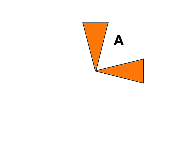
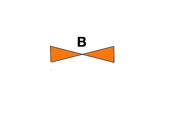
To illustrate the previous result, we give examples of sets AA and BB for which uA∈W2,∞u_{A}\in W^{2,\infty} and uB∉W2,∞u_{B}\not\in W^{2,\infty} in a small neighborhood of the origin, though they look very similar! This can be done by taking

A=Sα​(0)∪Sα​(π2)A=S^{\alpha}(0)\cup S^{\alpha}(\frac{\pi}{2})

and

B=Sα​(0)∪Sα​(π)B=S^{\alpha}(0)\cup S^{\alpha}(\pi)

which are pictured below. It is clear that AA satisfies the conditions of Theorem 6.2 while BB does not.

Refer to caption
Refer to caption
Figure 2. ψA∈W2,∞​(B12​(0))ψB∉W2,∞​(B12​(0))\psi_{A}\in W^{2,\infty}(B_{\frac{1}{2}}(0))\quad\quad\quad\quad\quad\quad\quad\quad\quad\quad\quad\quad\quad\,\,\,\,\,\,\,\psi_{B}\not\in W^{2,\infty}(B_{\frac{1}{2}}(0))\quad\quad\quad\quad\quad\quad

7. Acknowledgements

The author would like to thank Nader Masmoudi, Fang-Hua Lin, and In-Jee Jeong for helpful discussions and the NSF for its generous funding.

8. Appendix

In this section we give the computation of the non-smooth part of the solution of

Δ​ψ=χA\Delta\psi=\chi_{A}

when A=Sα​(0)A=S^{\alpha}(0) for any α>0\alpha>0.

Lemma 8.1.
∫01∫0c​y1log⁡|x−y|​d​y1​d​y2=c2​[x12+x221+c2−2​(c​x2+x11+c2)2]​log|x12+x22|+G\int_{0}^{1}\int_{0}^{cy_{1}}\log|x-y|dy_{1}dy_{2}=\frac{c}{2}\Big[\frac{x_{1}^{2}+x_{2}^{2}}{1+c^{2}}-2\Big(\frac{cx_{2}+x_{1}}{1+c^{2}}\Big)^{2}\Big]\log|x_{1}^{2}+x_{2}^{2}|+G

with G∈W2,∞​(B12​(0)).G\in W^{2,\infty}(B_{\frac{1}{2}}(0)).

Proof.

A useful fact for this computation is that the anti-derivative of log⁡(x2+A2)\log(x^{2}+A^{2}) with respect to xx is: x​log⁡(x2+A2)x\log(x^{2}+A^{2}) plus a Lipschitz function with Lipschitz constant which is independent of AA when 0≤A≤1.0\leq A\leq 1.

∫01∫0c​y1log|x−y|d​y1​d​y2=12​∫01∫0c​y1log⁡|(x1−y1)2+(x2−y2)2|​d​y1​d​y2\int_{0}^{1}\int_{0}^{cy_{1}}\log|x-y|dy_{1}dy_{2}=\frac{1}{2}\int_{0}^{1}\int_{0}^{cy_{1}}\log|(x_{1}-y_{1})^{2}+(x_{2}-y_{2})^{2}|dy_{1}dy_{2}
=12​∫01(y2−x2)​log⁡|(x1−y1)2+(x2−y2)2||0c​y1​d​y1+G1,=\frac{1}{2}\int_{0}^{1}(y_{2}-x_{2})\log|(x_{1}-y_{1})^{2}+(x_{2}-y_{2})^{2}|\Big|_{0}^{cy_{1}}dy_{1}+G_{1},

where G1G_{1} is a “good” term belonging to W2,∞W^{2,\infty}. Hence, up to a W2,∞W^{2,\infty} function and multiplication by a constant, the integral in question equals:

∫01(c​y1−x2)​log|(x1−y1)2+(x2−c​y1)2|d​y1+∫01x2​log⁡|(x1−y1)2+x22|​d​y1.\int_{0}^{1}(cy_{1}-x_{2})\log|(x_{1}-y_{1})^{2}+(x_{2}-cy_{1})^{2}|dy_{1}+\int_{0}^{1}x_{2}\log|(x_{1}-y_{1})^{2}+x_{2}^{2}|dy_{1}.

Now, notice that

(x1−y1)2+(x2−c​y1)2=(1+c2)​y12−2​y1​(c​x2+x1)+x12+x22(x_{1}-y_{1})^{2}+(x_{2}-cy_{1})^{2}=(1+c^{2})y_{1}^{2}-2y_{1}(cx_{2}+x_{1})+x_{1}^{2}+x_{2}^{2}
=(1+c2​y1−c​x2+x11+c2)2+x12+x22−(c​x2+x1)21+c2=(\sqrt{1+c^{2}}y_{1}-\frac{cx_{2}+x_{1}}{\sqrt{1+c^{2}}})^{2}+x_{1}^{2}+x_{2}^{2}-\frac{(cx_{2}+x_{1})^{2}}{1+c^{2}}
=(1+c2)​[(y1−c​x2+x11+c2)2+(x12+x22)​(1+c2)−(c​x2+x1)2(1+c2)2]=(1+c^{2})\Big[(y_{1}-\frac{cx_{2}+x_{1}}{1+c^{2}})^{2}+\frac{(x_{1}^{2}+x_{2}^{2})(1+c^{2})-(cx_{2}+x_{1})^{2}}{(1+c^{2})^{2}}\Big]

In particular,

x2​∫01log⁡|(x1−y1)2+(x2−c​y1)2|​d​y1x_{2}\int_{0}^{1}\log|(x_{1}-y_{1})^{2}+(x_{2}-cy_{1})^{2}|dy_{1}
=x2​∫01log⁡[(y1−c​x2+x11+c2)2+(x12+x22)​(1+c2)−(c​x2+x1)2(1+c2)2]​d​y1+G2=x_{2}\int_{0}^{1}\log\Big[(y_{1}-\frac{cx_{2}+x_{1}}{1+c^{2}})^{2}+\frac{(x_{1}^{2}+x_{2}^{2})(1+c^{2})-(cx_{2}+x_{1})^{2}}{(1+c^{2})^{2}}\Big]dy_{1}+G_{2}

with G2∈W2,∞G_{2}\in W^{2,\infty}. Then,

x2​∫01log⁡[(c​x2+x11+c2)2+(x12+x22)​(1+c2)−(c​x2+x1)2(1+c2)2]​d​y1x_{2}\int_{0}^{1}\log\Big[(\frac{cx_{2}+x_{1}}{1+c^{2}})^{2}+\frac{(x_{1}^{2}+x_{2}^{2})(1+c^{2})-(cx_{2}+x_{1})^{2}}{(1+c^{2})^{2}}\Big]dy_{1}
=x2​log⁡|(c​x2+x11+c2)2+(x12+x22)​(1+c2)−(c​x2+x1)2(1+c2)2|=x2​log⁡|x12+x22|+G3.=x_{2}\log\Big|(\frac{cx_{2}+x_{1}}{1+c^{2}})^{2}+\frac{(x_{1}^{2}+x_{2}^{2})(1+c^{2})-(cx_{2}+x_{1})^{2}}{(1+c^{2})^{2}}\Big|=x_{2}\log|x_{1}^{2}+x_{2}^{2}|+G_{3}.

So we see that

∫01(c​y1−x2)​log|(x1−y1)2+(x2−c​y1)2|d​y1+∫01x2​log⁡|(x1−y1)2+x22|​d​y1\int_{0}^{1}(cy_{1}-x_{2})\log|(x_{1}-y_{1})^{2}+(x_{2}-cy_{1})^{2}|dy_{1}+\int_{0}^{1}x_{2}\log|(x_{1}-y_{1})^{2}+x_{2}^{2}|dy_{1}
=c​∫01y1​log⁡|(x1−y1)2+(x2−c​y1)2|​d​y1=c\int_{0}^{1}y_{1}\log|(x_{1}-y_{1})^{2}+(x_{2}-cy_{1})^{2}|dy_{1}
=c​∫01y1​log⁡[(y1−c​x2+x11+c2)2+(x12+x22)​(1+c2)−(c​x2+x1)2(1+c2)2]​d​y1.=c\int_{0}^{1}y_{1}\log\Big[(y_{1}-\frac{cx_{2}+x_{1}}{1+c^{2}})^{2}+\frac{(x_{1}^{2}+x_{2}^{2})(1+c^{2})-(cx_{2}+x_{1})^{2}}{(1+c^{2})^{2}}\Big]dy_{1}.

Now we note that the antiderivative of x​log⁡|(x−b)2+A|x\log|(x-b)^{2}+A| is 12​(A2−b2+x2)​log⁡|(x−b)2+A|\frac{1}{2}(A^{2}-b^{2}+x^{2})\log|(x-b)^{2}+A| plus a Lipschitz function with Lipschitz constant independent of AA. Hence, computing, the integral we get:

c2​[x12+x221+c2−2​(c​x2+x11+c2)2]​log⁡|x12+x22|.\frac{c}{2}\Big[\frac{x_{1}^{2}+x_{2}^{2}}{1+c^{2}}-2\Big(\frac{cx_{2}+x_{1}}{1+c^{2}}\Big)^{2}\Big]\log|x_{1}^{2}+x_{2}^{2}|.

plus W2,∞W^{2,\infty} parts.

Now noting that c=cot⁡αc=\cot\alpha gives us the result. ∎

References

  • [1] H. Bahouri and J.-Y. Chemin, Équations de transport relatives á des champs de veceurs non-lipschitziens et mécanique des fluides. Arch. Rational. Mech, Anal. 127 (1994), no. 2, 159-181.
  • [2] H. Bahouri, J.-Y. Chemin, and R. Danchin. Fourier analysis and nonlinear partial differential equations, volume 343 of Grundlehren der Mathematischen Wissenschaften [Fundamental Principles of Mathematical Sciences]. Springer, Heidelberg, 2011.
  • [3] A. Bertozzi and P. Constantin. Global Regularity for Vortex Patches. Comm. Math. Phys. 1993.
  • [4] J.-Y.Chemin. Persistency of geometric structures in bidimensional incompressible fluids. Annales scientifiques de l’École normale supérieure. Volume 26. Issue 4. Page 517 - 542
  • [5] T.M. Elgindi. Propagation of Singularities for the 2d incompressible Euler equations. In preparation.
  • [6] T.M. Elgindi and I.J. Jeong. On Singular Vortex Patches. In preparation.
  • [7] D. Gilbard and N.S. Trudinger. Elliptic Partial Differential Equations of Second Order. Grundlehren, Vol. 224, Springer-Verlag, Berlin, 1983.
  • [8] Q. Han and F.H. Lin. Elliptic Partial Differential Equations. Courant Lecture Notes, Vol. 1.
  • [9] A. Kiselev and V. Sverak. Small scale creation for solutions of the incompressible two dimensional Euler equation Annals of Math, 2015.
  • [10] X. Xu. Fast growth of the vorticity gradient in symmetric smooth domains for 2D incompressible ideal flow arXiv preprint, 2014.
  • [11] T. Itoh, H. Miura, and T. Yoneda. The growth of the vorticity gradient for the two-dimensional Euler flows on domains with corners arXiv preprint, 2016.
  • [12] V. I. Yudovich. Non-stationary flows of an ideal incompressible fluid. u Z. Vy cisl. Mat. i Mat. Fiz., 3:1032–1066, 1963.