A sieve problem and its application

Let $\theta$ be an arithmetic function, $\theta:\mathbb{N}\to\mathbb{R}\cup\{\infty\}$. We write $\mathcal{B}$ (or $\mathcal{B}_{\theta}$) to denote the set of positive integers containing $n=1$ and all those $n\geq 2$ with prime factorization $n=p_{1}^{\alpha_{1}}\cdots p_{k}^{\alpha_{k}}$, $p_{1}<p_{2}<\ldots<p_{k}$, which satisfy

(1)

$$p_{j+1}\leq\theta(p_{1}^{\alpha_{1}}\cdots p_{j}^{\alpha_{j}})\qquad(0\leq j<k),$$

where $p_{1}^{\alpha_{1}}\cdots p_{j}^{\alpha_{j}}$ is understood to be $1$ when $j=0$. Let $B(x)$ (or $B_{\theta}(x)$) be the number of positive integers $n\leq x$ in $\mathcal{B}$. The following list shows some examples of $\theta$ and its corresponding set $\mathcal{B}$.

• •

  If $\theta(n)=2n$, then $\mathcal{B}$ is the set of integers with $2$-dense divisors, i.e. integers $n$ which have a divisor in every interval $[y,2y]$ for $1\leq y\leq n$ (see [4, 5, 9]).

• •

  If $\theta(n)=\sigma(n)+1$, where $\sigma(n)$ is the sum-of-divisors function, then $\mathcal{B}$ is the set of practical numbers, i.e. integers $n$ such that every $1\leq m\leq n$ can be written as a sum of distinct positive divisors of $n$ (see [4, 5, 9] and the references therein).

• •

  If $\theta(n)=n+1$, then $\mathcal{B}$ is the set of even $\varphi$-practical numbers, i.e. even integers $n$ such that the polynomial $X^{n}-1$ has a divisor in $\mathbb{Z}[X]$ of every degree from $1$ to $n$ (see [2, 7, 8]).

Building on earlier work by Tenenbaum [5] and Saias [4], we found [9, Theorem 1.2] that

$$B(x)\sim\frac{c_{\theta}x}{\log x}\qquad(x\to\infty),$$

for some positive constant $c_{\theta}$, provided $\theta(n)$ satisfies

$$\max(2,n)\leq\theta(n)\ll\frac{n\log 2n}{(\log\log 3n)^{1+\varepsilon}}\quad(n\geq 1),$$

for some $\varepsilon>0$. This applies to each of the three examples listed above.

In this note, our goal is to investigate the set $\mathcal{B}$ in general, without any restrictions on $\theta$. We will show that $\mathcal{B}$ always has a natural density (Theorem 1) and provide a criterion to determine whether this natural density is positive or zero (Theorem 2). We give estimates for $B(x)$ with explicit error terms, first without any assumptions on $\theta$ (Theorem 1), and then under certain conditions on the size of $\theta(n)$ (Corollary 1 and Theorem 3).

As an application, we consider the following set, related to the distribution of divisors. Let $\mathcal{D}$ be the set of positive integers containing $n=1$ and all those $n\geq 2$, whose divisors $1=d_{1}<d_{2}<\ldots<d_{\tau(n)}=n$ satisfy

(2)

$$d_{j+1}\leq\theta(d_{j})\qquad(1\leq j<\tau(n)).$$

We write $D(x)$ for the number of positive integers $n\leq x$ in $\mathcal{D}$. Theorem 4 shows that $\mathcal{B}=\mathcal{D}$ provided $\theta(n)/n$ is non-decreasing, so that all results concerning $B(x)$ also apply to $D(x)$ under this assumption.

Let $P^{+}(n)$ (resp. $P^{-}(n)$) denote the largest (resp. smallest) prime factor of $n\geq 2$ and put $P^{+}(1)=1$, $P^{-}(1)=\infty$.

Note that replacing $\theta(n)$ by $\max(\theta(n),P^{+}(n))$ in (1) leaves the set $\mathcal{B}$ unchanged, because of the assumption $p_{1}<p_{2}<\ldots<p_{k}$. Moreover, if $\theta(1)<2$ then $\mathcal{B}=\{1\}$. Thus, we may assume from now on, without any loss of generality, that

(3)

$$\theta:\mathbb{N}\to\mathbb{R}\cup\{\infty\},\quad\theta(1)\geq 2,\quad\theta(n)\geq P^{+}(n)\quad(n\geq 2).$$

Let $\chi(n)$ be the characteristic function of the set $\mathcal{B}$. We shall see in Lemma 4 that the series

$$L=\sum_{n\geq 1}\frac{\chi(n)}{n}\prod_{p\leq\theta(n)}\left(1-\frac{1}{p}\right)$$

converges to a value $0\leq L\leq 1$. Theorem 1 shows that, for every choice of $\theta$, the set $\mathcal{B}$ has a natural density, which is given by $1-L$.

Theorem 2 provides a simple criterion to determine whether $L=1$ and $B(x)=o(x)$, or $L<1$ and $B(x)\sim(1-L)x$.

Note that the three examples of $\theta$ listed in the introduction satisfy $L=1$ and $B(x)=o(x)$. For an instance where $L<1$, consider $\theta(n)=2^{n}$, for which $L=0.7734...$ by numerical computation. (For $n\geq 30$ we used estimates for the Euler product with effective error bounds due to Rosser and Schoenfeld [3, Theorem 7].) Hence (4) implies that $B(x)=cx(1+o(1))$ with $c=1-L=0.2265...$, while (5) shows that we have $B(x)=cx(1+O(1/\log x))$, when $\theta(n)=2^{n}$.

Corollary 1 generalizes this example to $\log\theta(n)\asymp n^{a}$, where $a$ is a positive constant. We also consider the case $\log\theta(n)\asymp(\log 2n)^{a}$, where $a>1$ is constant. (The notation $f(n)\asymp g(n)$ means that $f(n)\ll g(n)$ (i.e. $f(n)=O(g(n))$) and $g(n)\ll f(n)$.)

The error terms in Corollary 1 are easily derived from (5), using the trivial bound $\chi(n)\leq 1$. The claim that $0<L<1$ follows directly from Theorem 2, with (i) $f(n)=\max(2,\exp(cn^{a}))$ and (ii) $f(n)=\max(2,\exp(c(\log 2n)^{a}))$, where $c>0$ is a suitable constant. Other examples of $\theta$, for which $L<1$, can be dealt with similarly.

When $B(x)=o(x)$, we need a different strategy for obtaining an asymptotic formula for $B(x)$, since the estimate (5) provides only an upper bound for $B(x)$ whenever $L=1$. We will focus on the case $\theta(n)\asymp n^{a}$, where $a\geq 1$ is constant. Theorem 2 shows that $L=1$ and $B(x)=o(x)$. Theorem 3 generalizes [9, Theorem 1.2], where the case $a=1$ is established with $\lambda_{1}=1$.

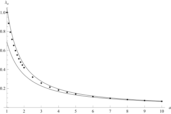
Figure 1 and Table 1 show several values of $\lambda_{a}$, obtained by solving equation (7) numerically.

As in [9, Theorem 1.2] with $a=1$, one can consider a less restrictive condition on $\theta$, such as $n^{a}(\log n)^{-b}\ll\theta(n)\ll n^{a}(\log n)^{b}$, where $0\leq b<1$, and establish the estimate (6) with the relative error term $O(1/\log x)$ replaced by $O(1/(\log x)^{1-b})$. However, we will not pursue this here.

We now turn to the distribution of divisors. Let $\mathcal{D}$ be the set defined in (2). When $\theta(n)=tn$, where $t$ is constant, Tenenbaum [5, Lemma 2.2] showed that $\mathcal{D}=\mathcal{B}$. We want to generalize this result as much as possible. The example $\theta(n)=n+1$, for which $\mathcal{D}=\{1,2\}$ while $\mathcal{B}$ is infinite, illustrates that some condition on $\theta$ is required to ensure equality of these two sets. The condition we need is

(10)

$$\theta(n)\leq\theta(n+1),\quad m\theta(n)\leq\theta(mn)\qquad(n,m\geq 1,\ \gcd(n,m)=1).$$

Note that (10) is satisfied if $\theta(n)/n$ is non-decreasing.

As an example, consider $\theta(n)=n^{2}+1$. Theorems 3 and 4 show that the number of integers $n\leq x$ whose divisors $1=d_{1}<d_{2}<\ldots<d_{\tau(n)}=n$ satisfy $d_{j+1}\leq d_{j}^{2}+1$ for $1\leq j<\tau(n)$, is given by

$$D(x)=\frac{cx}{(\log x)^{\lambda_{2}}}\left(1+O\left(\frac{1}{\log x}\right)\right),$$

where $c$ is a positive constant and $\lambda_{2}=0.4191...$

With $\theta(n)=2^{n}$, Corollary 1 and Theorem 4 show that the number of integers $n\leq x$ whose divisors $1=d_{1}<d_{2}<\ldots<d_{\tau(n)}=n$ satisfy $d_{j+1}\leq 2^{d_{j}}$ for $1\leq j<\tau(n)$, is given by

$$D(x)=(1-L)x\left(1+O\left(\frac{1}{\log x}\right)\right),$$

where $1-L=0.2265...$

The proof of Theorem 1 is based on the functional equation in Lemma 3 and an estimate for the number of integers without small prime factors in Lemma 2. Theorem 2 is established with the help of Theorem 1. The proof of Theorem 3, which requires the most amount of work, is modeled after [9, Theorem 1.2], with the added difficulty that the poles of the Laplace transform (i.e. the solutions of equation (7)) now depend on the parameter $a$ (see Lemma 9). The proof of Theorem 4 generalizes that of Tenenbaum [5, Lemma 2.2].

Let

$$\Phi(x,y)=\#\big\{1\leq n\leq x:P^{-}(n)>y\big\}$$

and define $\Phi(x,\infty)=1$ for $x\geq 1$. For $u\geq 1$, Buchstab’s function $\omega(u)$ is defined as the unique continuous solution to the equation

$$(u\omega(u))^{\prime}=\omega(u-1)\qquad(u>2)$$

with initial condition $u\omega(u)=1$ for $1\leq u\leq 2$. Let $\omega(u)=0$ for $u<1$ and define $\omega$ at 1 and $\omega^{\prime}$ at 1 and 2 by right-continuity. Let $\Gamma(u)$ denote the usual gamma function.

The calculation of the values of $\lambda_{a}$ in Table 1 and the approximation of several integrals in the proof of Lemma 9 require estimates for integrals involving $\omega(t)-e^{-\gamma}$. For that purpose, we used exact formulas for $\omega(t)$ for $0\leq t\leq 5$, derived with the help of Mathematica. To estimate the contribution from $t>5$, we used a table of zeros and relative extrema of $\omega(t)-e^{-\gamma}$ on the interval $[5,10.3355]$ due to Cheer and Goldston [1], and the estimate (ii) from Lemma 1 for $t\geq 10.3355$.

Throughout this section, we assume that $\theta$ satisfies (3) and that

(11)

$$B(x)\ll\frac{x}{(\log x)^{\nu}}\qquad(x\geq 2),$$

for some suitable $\nu\in[0,1]$, to be determined later. Clearly, $\nu=0$ is admissible. All constants implied by $\ll$ and the big O notation may depend on $\theta$, and therefore on $a$, but are otherwise absolute. Lemmas 5 through 8 correspond to Lemmas 5.3 through 5.7 of [9]. The main difference is the assumption on the size of $B(x)$ for the purpose of estimating the error terms, for which we use (11) here.

From Lemma 8 we have, for $x\geq e$,

(13)

$$B(x)=x\,\alpha-x\int_{e}^{\infty}\frac{B(y)}{ay^{2}\log y}\,\omega\left(\frac{\log x/y}{a\log y}\right)\mathrm{d}y+O\left(\frac{x}{(\log x)^{1+\nu}}\right),$$

where

$$\alpha:=e^{-\gamma}\int_{e}^{\infty}\frac{B(y)}{ay^{2}\log y}\,\mathrm{d}y.$$

For $x\geq e$ let $z\geq 0$ be given by

$$z=\log\log(x)$$

and let

$$G_{\theta}(z):=\frac{B\left(\exp(e^{z})\right)}{\exp(e^{z})}=\frac{B(x)}{x}.$$

Dividing (13) by $x$ and changing variables in the integral via $u=\log\log y$ we get, for $z\geq 0$,

(14)

$$\begin{split}G_{\theta}(z)&=\alpha-\frac{1}{a}\int_{0}^{z}G_{\theta}(u)\,\omega\left((e^{z-u}-1)/a\right)\,\mathrm{d}u+E_{\theta}(z)\\ &=\alpha-\frac{1}{a}\int_{0}^{z}G_{\theta}(u)\,\Omega_{a}(z-u)\,\mathrm{d}u+E_{\theta}(z),\end{split}$$

where

(15)

$$E_{\theta}(z)\ll e^{-(1+\nu)z}$$

and

$$\Omega_{a}(u):=\omega\left((e^{u}-1)/a\right).$$

Equation (14) leads to the equation of Laplace transforms

$$\widehat{G}_{\theta}(s)=\frac{\alpha}{s}-\frac{1}{a}\widehat{G}_{\theta}(s)\,\widehat{\Omega}_{a}(s)+\widehat{E}_{\theta}(s)\qquad(\re s>0),$$

which we solve for $\widehat{G}_{\theta}(s)$ to get

$$\widehat{G}_{\theta}(s)=\frac{\alpha}{s(1+\frac{1}{a}\widehat{\Omega}_{a}(s))}+\frac{\widehat{E}_{\theta}(s)}{1+\frac{1}{a}\widehat{\Omega}_{a}(s)}\qquad(\re s>0).$$

Let $F_{a}(z)$ be given by

(16)

$$F_{a}(z)=1-\frac{1}{a}\int_{0}^{z}F_{a}(u)\,\Omega_{a}(z-u)\,\mathrm{d}u.$$

Equation (16) is an error-free, rescaled version of equation (14), which depends on $a$, but does not involve $\theta$. Note that the upper limit of the integral could be replaced by $z-\log(a+1)$, since $\omega(t)=0$ for $t<1$. Thus $F_{a}(z)=1$ for $0\leq z\leq\log(a+1)$, and for $z>\log(a+1)$, $F_{a}(z)$ is determined by the values of $F_{a}(u)$ for $u\in[0,z-\log(a+1)]$. Hence (16) defines the continuous function $F_{a}(z)$ for $z\geq 0$. As with $G_{\theta}(z)$, we find that the Laplace transform of $F_{a}(z)$ is given by

$$\widehat{F}_{a}(s)=\frac{1}{s(1+\frac{1}{a}\widehat{\Omega}_{a}(s))}\qquad(\re s>0),$$

and therefore,

(17)

$$\widehat{G}_{\theta}(s)=\alpha\widehat{F}_{a}(s)+s\widehat{F}_{a}(s)\widehat{E}_{\theta}(s).$$

The Laplace transform of $\Omega_{a}(u)$, defined for $\re(s)>0$, is given by

$$\begin{split}\widehat{\Omega}_{a}(s)&=\int_{0}^{\infty}\omega((e^{u}-1)/a)\,e^{-us}du=a\int_{0}^{\infty}\omega(t)\frac{dt}{(at+1)^{s+1}}\\ &=\frac{e^{-\gamma}}{s(a+1)^{s}}+a\int_{1}^{\infty}\bigl(\omega(t)-e^{-\gamma}\bigr)\frac{dt}{(at+1)^{s+1}}.\end{split}$$

The last equation extends $\widehat{\Omega}_{a}(s)$ to a meromorphic function on $\mathbb{C}$ with a simple pole at $s=0$. We will need to investigate the location of zeros of the entire function $g_{a}(s)$, defined by

$$\begin{split}g_{a}(s)&=1/\widehat{F}_{a}(s)=s\left(1+\frac{1}{a}\widehat{\Omega}_{a}(s)\right)\\ &=s+\frac{e^{-\gamma}}{a(a+1)^{s}}+s\int_{1}^{\infty}\bigl(\omega(t)-e^{-\gamma}\bigr)\frac{dt}{(at+1)^{s+1}}.\end{split}$$