Conformal perturbation of off-critical correlators in the 3D Ising universality class
Abstract
Thanks to the impressive progress of conformal bootstrap methods we have now very precise estimates of both scaling dimensions and OPE coefficients for several 3D universality classes. We show how to use this information to obtain similarly precise estimates for off-critical correlators using conformal perturbation. We discuss in particular the , and two point functions in the high and low temperature regimes of the 3D Ising model and evaluate the leading and next to leading terms in the expansion, where is the reduced temperature. Our results for agree both with Monte Carlo simulations and with a set of experimental estimates of the critical scattering function.
I Introduction
Our understanding of critical phenomena in three dimensions has been greatly improved in the past few years by the remarkable progress of the Conformal Bootstrap program. In particular, using Conformal Bootstrap techniques, very precise estimates of scaling dimensions and Operator Product Expansion (OPE) coefficients could be obtained for several three dimensional models [1, 2, 3, 4, 5, 6, 7] . Among them a particular attention was devoted to the 3D Ising model, which plays somehow a benchmark role in this context, since in this case both high precision Monte Carlo results [8, 9, 10] and accurate experimental estimates [11] exist for these quantities.
The aim of this letter is to leverage the accurate knowledge of the model that we have at the critical point to predict the behaviour of off-critical correlators in the whole scaling region using Conformal Perturbation Theory (CPT). We shall discuss, as an example, the thermal perturbation of the , and correlators in the 3D Ising model both above and below the critical temperature, but our results are of general validity and may be applied to any model for which scaling dimensions and critical OPE constants are known with sufficient precision. In this sense our work is a natural extension of the Conformal Bootstrap Approach.
It is important to stress the role played by Conformal Symmetry in our analysis. In fact the general form of correlation functions and in particular their dependence on the expansion parameter (in our case the reduced temperature ) was already understood more than fifty years ago [12, 13] and can be easily obtained using standard scaling arguments valid in general for any critical point. The additional bonus we have in the case of a conformally invariant critical point is that the terms appearing in the CPT expansion can be related to the derivatives of the Wilson coefficients, calculated at the critical point [14, 15, 16, 17]. In several cases these derivatives can be evaluated exactly and only depend on the critical indices and OPE coefficients of the underlying Conformal Field Theory (CFT). Unfortunately the power of this approach is limited by the fact that the vacuum expectation values (VEVs) of the relevant operators which appear in the expansion must be known to all orders in the perturbation parameter. This means in practical applications that they appear in the CPT expansion as external inputs, they are not universal and in general cannot be fixed by using CFT data. In some cases (in particular in two dimensions and for integrable perturbations) these VEVs can be evaluated analytically [15, 16, 17] or numerically using the truncated conformal space method [18]. When this is not possible they must be evaluated using independent non-perturbative methods, like strong coupling expansions or Monte Carlo simulations. There are however exceptions to this rule. The terms involving derivatives of the Wilson coefficients of the type do not require any external information, they can be evaluated exactly (we shall see below an example) and represent thus true, universal, testable predictions of the CPT approach. In this sense they are more informative than usual universal amplitudes ratios since they test the presence of the whole conformal symmetry in the critical theory and not only of scale invariance, that is, instead, a sufficient requirement to construct ordinary universal amplitude ratios.
The main goal of this paper is exactly to perform this non trivial ”conformality test” in the case of the 3D Ising model. As a side result of this analysis we shall be able to give a very precise prediction for the scaling behaviour of the correlator in the scaling region which we shall successfully compare both with Monte Carlo results and with a set of experimental estimates of the critical scattering function for a sample at critical density.
II Thermal perturbation theory
Let us consider the thermal perturbation of the 3D Ising model, characterized by two relevant operators, the magnetization and the energy , whose dimensions are and respectively [6, 7].
The perturbed action is given by the conformal point action , plus a term proportional to the energy operator:
| (1) |
where is a parameter related in the continuum limit to the deviation from the critical temperature. We shall denote in the following with expectation values with respect to the perturbed action and with those with respect to the unperturbed conformal invariant action .
In [15] the correlators of two generic operators and of the perturbed CFT were expressed, by using the operator product expansion, in terms of the Wilson coefficients, calculated outside of the critical point:
| (2) |
In order to perform the CPT expansion one has to expand in a Taylor series the Wilson coefficients, while the VEV’s must be determined in a non perturbative way. The first few terms of this CPT expansion read
| (3) |
where denotes the derivatives of the Wilson coefficients with respect to evaluated at the critical point.
In [14] it was shown how to calculate these derivatives to any order and it was proved that they are infrared finite.
Defining , the perturbed one-point functions are (see [19] for definitions and further information on the scaling behaviour of the model):
| (4) |
We have the following expression for the first three orders of perturbed two-point function of :
| (5) |
To make contact with the usual definition for the structure constants we factorize the dependence in the Wilson coefficients:
Following [14] we can write the derivatives of the Wilson coefficient as:
| (6) |
The three point function reads:
while . and the second term in the integral acts as an infrared counterterm. The integral (6) can be calculated using a Mellin transform technique (see [20]) or numerically. In the first case only the first term gives a contribution:
where . It is convenient to define , so after performing the angular integrals we get:
which can be solved in terms of Gamma functions giving as a final result: .
Now we can write, introducing the scaling variable , the following expression for the perturbed two-point function:
| (7) |
Proceeding in the same way we have for the others correlators of interest:
| (8) |
| (9) |
This is the main result of our paper. It is interesting to compare these quantities with the second terms in the CPT expansions. To estimate these terms we need the values of the which can be easily obtained from the very precise estimates of their lattice values reported in [8] , and the lattice to continuum conversion constants , [9, 10]. We find and to which correspond the following values for the terms which appear in the CPT expansion:
Thus we see that, in the range of value of of experimental interest, the third term in the CPT expansion is of the same size of the second one and cannot be neglected in the correlators. Moreover we shall see below, by comparing with Monte Carlo simulations that, in the same range, the sum of these two terms almost saturates the correlator, i.e that the higher order terms neglected in the above expansion give a contribution to the correlator almost negligible (and in any case never larger than ) with respect to the first three terms. They can thus be safely neglected when comparing with the experimental results. On the contrary, within the precision of the experimental data, both the second and the third term of the CPT expansion are necessary to fit the data.
III Monte Carlo simulations
We compared our results with a set of Monte Carlo simulations of the Ising model using the standard nearest neighbour action for which the critical temperature is known with high precision [8]. The temperature perturbation from the critical point is defined through the parameter . With this convention in the high temperature phase we have . We performed our simulations with a standard Metropolis updating and multispin coding technique on a cubic lattice with periodic boundary conditions. We fixed the lattice size , which was the maximum value compatible with the computational resources at our disposal. We evaluated the correlators for many distances in different simulations, so our data are uncorrelated, and we sampled about configurations for each simulation, with a thermalization time of sweeps.
We defined the lattice discretization of the spin and energy operators as:
where is the energy analytic part that must be subtracted. Also is known in the Ising case with high precision: , where and are respectively the energy and the specific heat at the bulk [8].
We chose small enough so as to have a large enough value of the correlation length , but not too small in order to avoid finite size effects. The optimal choice turned out to be , for which lattice spacings in the high temperature phase and lattice spacings for low temperatures. We verified that the finite size effects were negligible within our current precision for these temperatures.
The results of our simulations are reported together with the CPT expansion in fig.1. We also report the prediction truncated at the second order. It is easy to see that the universal third term of the expansion that we evaluate in this letter gives a large contribution to the correlator, which cannot be neglected within the precision of current data (and also, as we shall see, within the precision of experimental estimates), and that our complete CPT expansion agrees remarkably well with Monte Carlo data.
In order to estimate the contribution of the higher order terms neglected in the CPT expansions of eq.s(7,8,9) we fitted the spin-spin correlator with eq. (7), keeping the coefficient of the last term (i.e. ) as a free parameter.
The results of the fits are reported in tab.1 where we quoted separately statistical and systematic (mainly due to the uncertainty in and ) errors. The results, for all temperatures both above and below , turn out to be remarkably close to the theoretical prediction thus showing that in this range of values of the scaling variable higher order terms in the CPT expansion are almost negligible, as also suggested by fig.1.
| 6 | 20 | 61.4 (0.9)[1.2] | 0.7 | |
| 6 | 20 | 60.9 (0.9)[1.5] | 0.8 | |
| 7 | 14 | 61.3 (0.8)[1.0] | 1.0 | |
| 8 | 20 | 61.1 (0.9)[1.8] | 1.1 | |
| 6 | 13 | 61.0 (0.8)[1.0] | 0.7 | |
| 8 | 20 | 61.6 (0.7)[1.5] | 1.2 |
IV Scattering Function and Comparison with experimental results
By Fourier transforming the spin-spin correlator it is easy to construct the Scattering Function (for a detailed discussion see for instance [21]) which turns out to have exactly the form predicted by Fisher and Langer [12]
| (10) |
with , where is the momentum-transfer vector and the correlation length. The coefficients of the expansion can be deduced exactly from the CPT analysis discussed above:
where and are numerical coefficients coming from the Fourier transform of the power law terms of eq.(7). Combining all the factors we finally obtain:
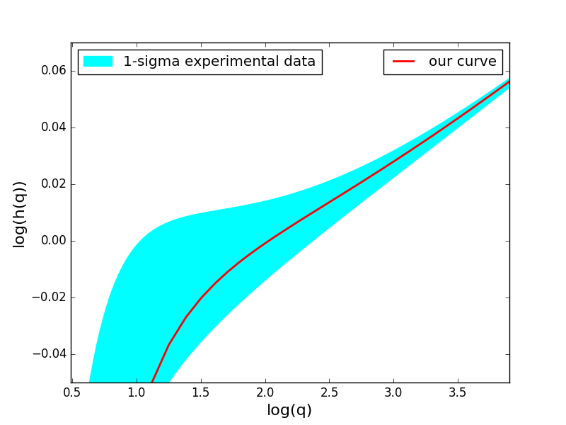
This result allows a set of interesting theoretical end experimental checks. First of all they agree remarkably well with the results obtained in[21] with the -expansion within the Bray approximation [22] (see tab.2). They also show that the Bray approximation which assumes is indeed a good approximation of the CPT result which gives . This is reassuring, since it shows that (as we would expect) the -expansion actually ”knows” that the 3D Ising model is conformally invariant. As expected they also agree with the Fourier Transform of our Monte Carlo results (see the first column of tab.2). What is more interesting is that they also agree with a set of experimental measures of the scattering function obtained from a small-angle neutron scattering experiment on a sample of at critical density [11]. We report our result together with the experimental estimates in fig.2 where we plotted the scattering function in a log-log scale so as to show the large scaling behaviour as a straight line and normalized it (as usual) to the Ornstein-Zernicke (OZ) function: so as to evidentiate the large deviations with respect to the OZ behaviour (which describes the small behaviour of the scattering function). We plot our results with a red line and in light blue the region of uncertainty quoted in [11] as the best fit result of their experimental scattering data within the Bray approximation. We report their best fit estimates for , in the last column of tab.2, together with the results from our conformal perturbation theory, the MC simulations, and the estimates obtained via -expansion in [21].

| MC | CPT | -exp | experim. | |
|---|---|---|---|---|
| 2.54 (2) | 2.56 | 2.05 (80) | ||
| -1.86 (1) | -1.3 | -1.5 (8) | ||
| -3.42 (6) | -3.64 (1) | -3.46 | -2.95 (80) | |
| 1.20 (2) | 1.28 (1) | 0.9 | 1.0 (8) |
V Conclusions
Our main goal in this letter was to extend the knowledge reached in these last years on higher dimensional CFTs to the off-critical, scaling, regime of the models. We concentrated in particular on two point functions in the 3D Ising model perturbed by the thermal operator, but we see no obstruction to extend this program to other universality classes or to three-point functions. An important aspect of our analysis was the identification of a set of terms in the CPT expansion which are universal as a consequence of the conformal symmetry of the underlying fixed point theory. These universal amplitude combinations were already discussed, and compared with two-dimensional data, in [23]. Our results are in good agreement both with Monte Carlo simulations and with a set of experimental results in systems belonging to the 3D Ising universality class. We think that in future these techniques will allow us to vastly extend our ability to describe experimental data in the scaling regime of three dimensional critical points.
Acknowledgments: We would like to thank A. Amoretti, F. Gliozzi, M. Panero, A Pelissetto and E. Vicari for useful discussions and suggestions and the INFN Pisa GRID data center for supporting the numerical simulations.
References
- [1] S. El-Showk et al., Phys. Rev. D86, 025022 (2012), 1203.6064.
- [2] S. El-Showk et al., J. Stat. Phys. 157, 869 (2014), 1403.4545.
- [3] F. Gliozzi, Phys. Rev. Lett. 111, 161602 (2013), 1307.3111.
- [4] F. Gliozzi and A. Rago, JHEP 10, 042 (2014), 1403.6003.
- [5] F. Kos, D. Poland, D. Simmons-Duffin, and A. Vichi, JHEP 11, 106 (2015), 1504.07997.
- [6] Z. Komargodski and D. Simmons-Duffin, (2016), 1603.04444.
- [7] F. Kos, D. Poland, D. Simmons-Duffin, and A. Vichi, (2016), 1603.04436.
- [8] M. Hasenbusch, Phys. Rev. B85, 174421 (2012), 1202.6206.
- [9] M. Caselle, G. Costagliola, and N. Magnoli, Phys. Rev. D91, 061901 (2015), 1501.04065.
- [10] G. Costagliola, Phys. Rev. D93, 066008 (2016), 1511.02921.
- [11] P. Damay, F. Leclercq, R. Magli, F. Formisano, and P. Lindner, Phys. Rev. B58, 12038 (1998).
- [12] M. E. Fisher and J. S. Langer, Phys. Rev. Lett. 20, 665 (1968).
- [13] E. Brezin, D. J. Amit, and J. Zinn-Justin, Phys. Rev. Lett. 32, 151 (1974).
- [14] R. Guida and N. Magnoli, Nucl. Phys. B471, 361 (1996), hep-th/9511209.
- [15] R. Guida and N. Magnoli, Int. J. Mod. Phys. A13, 1145 (1998), hep-th/9612154.
- [16] M. Caselle, P. Grinza, and N. Magnoli, J. Phys. A34, 8733 (2001), hep-th/0103263.
- [17] M. Caselle, P. Grinza, and N. Magnoli, Nucl. Phys. B579, 635 (2000), hep-th/9909065.
- [18] R. Guida and N. Magnoli, Phys. Lett. B411, 127 (1997), hep-th/9706017.
- [19] A. Pelissetto and E. Vicari, Phys. Rept. 368, 549 (2002), cond-mat/0012164.
- [20] R. Guida and N. Magnoli, Nucl. Phys. B483, 563 (1997), hep-th/9606072.
- [21] V. Martin-Mayor, A. Pelissetto, and E. Vicari, Phys. Rev. E66, 026112 (2002), cond-mat/0202393.
- [22] A. J. Bray, Phys. Rev. B14, 1248 (1976).
- [23] M. Caselle, P. Grinza, R. Guida, and N. Magnoli, J. Phys. A37, L47 (2004), hep-th/0306086.