Complex Analysis of Askaryan Radiation: A Fully Analytic Treatment including the LPM effect and Cascade Form Factor

The challenge of detecting UHE-$\nu$ with ARA/ARIANNA is one of distinguishing natural RF pulses from backgrounds. Every RF antenna observes thermal radiation associated with the temperature of the observed medium. ARA/ARIANNA background rates are a mixture of thermal radiation from ice, the sky, and the Milky Way [Barwick201512] [Allison2012457] [PhysRevD.93.082003]. Thermal noise is uncorrelated with digital signal templates generated by convolving theoretical Askaryan pulses with detector response. Signal templates have been used recently to detect UHECR with the ARIANNA Hexagonal Radio Array (HRA) [Barwick201750]. More significantly, vibrational signal templates were used to detect gravitational wave signals in the Advanced LIGO detector [PhysRevLett.116.061102]. In each case, a template library was created, in which individual templates share a physical origin, but use different functional parameters that span parameter-space.

Creating template libraries with semi-analytic and fully analytic models is far more efficient than creating them with particle MC codes. The Askaryan field is derived in semi-analytic models from cascade profiles computed via MC codes, accounting for stochastic effects in cascade profiles [PhysRevD.61.023001]. Fully analytic models are derived mathematically, where every model parameter has a physical origin and explanation. Template libraries may then be generated by tuning continuously parameters, accounting for regions of parameter-space where the form factor $\widetilde{F}(\omega,\theta)$ and LPM elongation dominate. Although the resulting template library would not account for stochastic processes, it would contain the effects of the form factor and LPM elongation, which control the sensitivity and design of Antarctic detectors. Examples of parameter-space variables are: the range to the interaction $R$, the frequencies $\nu$, the length of the cascade $a$, the viewing angle $\theta$, the fraction of the cascade that is electromagnetic or hadronic, the total cascade energy $E_{\rm C}$, and the lateral width of the cascade $\sqrt{2\pi}\rho_{\rm 0}$.

The conventions are taken from Sec. 2 to build the RB model in the code [PhysRevD.65.016003]. RB derive the Askaryan fields from Maxwell’s equations in the Lorentz gauge for a dielectric medium, by expanding with a special scalar parameter $\eta$. The source current, $\mathbf{J}(t^{\prime},\textbf{x}^{\prime})$, is described by an ICD $f(z^{\prime}-vt,\textbf{$\rho$}^{\prime})$, excess charge profile $n(z^{\prime})$, and cascade speed $\mathbf{v}$:

The function $f(z^{\prime}-vt,\textbf{$\rho$}^{\prime})$ is the 3D ICD. Equation 5 is the squared ratio of $a$, and $\Delta z_{\rm coh}$, the longitudinal range where the Askaryan radiation must be coherent. To understand $\Delta z_{\rm coh}$, consider Feyman’s formula [PhysRevD.45.362]. Radiation from an accelerating point charge is proportional to the angular acceleration $\ddot{\theta}$ relative to the observer. The coherence regime is defined by $|z^{\prime}|\lesssim\Delta z_{\rm coh}$, where $\ddot{\theta}$ and $R(z^{\prime})$ are constant in time to first order, and $\ddot{\theta}$ is maximized. RB show that if $\Delta R(z^{\prime})<\lambda$ in this limit, $\Delta z_{\rm coh}<(R/(k\sin^{2}\theta))^{1/2}$.

The dominant Askaryan radiation occurs when $|z^{\prime}|\lesssim\Delta z_{\rm coh}$. In the Fresnel and Fraunhofer (far-field) regimes, $\eta<1$. The calculations, however, are valid for any $\eta$, rather than only the in the far-field ($\eta\rightarrow 0$, and $kR\gg 1$, $R\gg a$). If $a\ll\Delta z_{\rm coh}$, then the fields have spherical symmetry, and the limit $kR\gg 1$ corresponds to the far-field. Conversely, if $a\gg\Delta z_{\rm coh}$, then $\eta\rightarrow\infty$, the fields have cylindrical symmetry.

The longitudinal cascade width $a$, and therefore $\eta$, is derived in the code from either the Greisen (electromagnetic) or Gaisser-Hillas (hadronic) cascade profile functions (Secs. 3.4-3.4.1), and can be elongated by the LPM effect. The associated code requires the type of cascade profile (hadronic or electromagnetic) as an input, and whether the LPM effect must be applied. If the user specifies a purely hadronic cascade, no further action is taken if the LPM effect is activated [PhysRevD.61.023001].

RB insert the vector current $\textbf{J}(t^{\prime},\textbf{x}^{\prime})$ into Maxwell’s equations, and solve for the vector potential:

RB then define $R(z^{\prime})=\sqrt{(z-z^{\prime})^{2}+\rho^{2}})$, and expand around $\rho^{\prime}=0$:

In Eq. 7, the third term on the right-hand side is dropped, because $\rho^{\prime}\ll R(z^{\prime})$. The vector potential in Eq. 6 is then factored into the form factor $\widetilde{F}(\omega)$ and a vector potential. $\widetilde{F}(\omega)$ is the three-dimensional Fourier transform of the ICD, and the vector potential is governed by $n(z^{\prime})$. Thus, $\widetilde{F}(\omega)$ describes the charge distribution, and the vector potential describes the charge evolution. Equations 8-9 summarize the result. In Eqs. 8-9, $\mathbf{\widetilde{A}}^{FF}$ is the vector potential, named the Fresnel-Fraunhofer (FF) potential in RB.

Equations 10-13 express the general RB result for the electric field $\textbf{E}=-\partial\textbf{A}/\partial t$, in terms of the frequency $\nu$, viewing angle $\theta$, and $\eta$:

Equation 10 is the total field, with an overall phase factor defined in Eq. 11. Equation 12 contains the vector structure, and Eq. 13 governs the phase and angular structure.

The Landau-Pomeranchuk-Migdal (LPM) effect is a suppression of the pair-creation and bremsstrahlung cross-sections at cascade energies above a material-dependent constant known as the LPM energy or $E_{\rm LPM}$ [RevModPhys.71.1501]:

In Eq. 14, $m$ is the electron mass, $\alpha$ is the fine-structure constant, and $X_{\rm 0}$ is the radiation distance ($E_{\rm LPM}=0.303$ PeV for ice). If $E_{\rm C}>E_{\rm LPM}$, the quantum mechanical formation length of these interactions is longer than atomic separations, leading to quantum interference and suppressing cross-sections. The result is a longitudinal shower elongation, from the non-interacting, higher-energy particles. The LPM effect is reviewed by S.R. Klein in Ref. [RevModPhys.71.1501].

The LPM changes how the RB model must be applied. Under normal circumstances, the quantity $n_{\rm max}a$ approximates the area under the cascade profile for particles with energy greater than some critical energy: $n_{\rm max}a\propto E_{\rm C}$. It is shown in Ref. [101103physrevd82074017] that in the LPM-regime, $a\propto\sqrt{E_{\rm C}/E_{\rm crit}}$. While it may appear that changing the energy scaling of $a$ violates energy conservation through the field normalization $n_{\rm max}a$, this is not necessarily the case.

First, the amount of radiated energy does not have to track the total energy, if the cascade shape is modified. The Frank-Tamm radiation distribution for a charge moving through a track of length $L$ states: $d^{2}P/d\Omega d\omega\propto L^{2}$ [PhysRevD.65.016003]. The LPM effect would increase $L$, increasing the radiated energy. The increase is contingent on $L$ remaining comparable to $\Delta z_{\rm coh}$, avoiding spectral cut-off. It is shown in Sec. 3.6 (graphically) and Sec. 4 (mathematically) that enhancements due to cascade elongation are attenuated by a combination of decoherence, $\widetilde{F}$, and narrowed Cherenkov cone-width.

Second, it should not be assumed naively that $n_{\rm max}$ must be decreased in direct proportion to the increase in $a$, under LPM elongation. Absent the LPM effect, the inverse relationship between $a$ and $n_{\rm max}$ merely reflects that $E_{\rm C}$ is a constant, with $\approx 10^{-7}$ of the energy in TeV passing to Askaryan radiation in V/m/MHz. Figures 12-13 of Ref. [Cillis_Influence_1999] demonstrate LPM elongation, but $n_{\rm max}$ is not reduced in direct proportion to $a$. Figure 12 of Ref. [Cillis_Influence_1999] shows that $X_{\rm max}$ grows and fluctuates at energies above $E_{\rm LPM}$. However, Fig. 13 of Ref. [Cillis_Influence_1999] shows that the energy-dependence of $n_{\rm max}$ stays approximately the same, and $n_{\rm max}$ fluctuates mildly. Further, Fig. 3 of [PhysRevD.61.023001] suggests that charged-current induced cascades, with mixed hadronic and electromagnetic components, have no reduction in $n_{\rm max}$ relative to neutral-current induced cascades, for which the LPM effect is not relevant [AlvarezMuniz1998396].

Physically, all particle energies must decrease below $E_{\rm LPM}$ eventually. This takes place before the cascade maximum, so to first order $n_{\rm max}$ is still governed by non-LPM physics, even if $E_{\rm C}>E_{\rm LPM}$. Conversely, ZHS and others have shown that the radiated field strength below 500 MHz is proportional to the weighted, projected track length of charged particles [PhysRevD.45.362]. The LPM effect cannot enhance dramatically the weighted projected track length, because the number of LPM-elongated tracks is a small fraction of the total number. The associated code contains a flag (strictLowFreqLimit) which directs the model to retain this limit by inversely scaling $n_{\rm max}$ in direct proportion to the increase in $a$. Requiring this limit is equivalent to stating that sub-showers with $E<E_{\rm LPM}$ occur both before and after cascade maximum, smearing $n(z^{\prime})$. From the arguments and references above, this is the most conservative approach.

Finally, S.R. Klein notes in Ref. [RevModPhys.71.1501] that the LPM effect may influence $\widetilde{F}(\omega,\theta)$. The lateral ICD is influenced by multiple scattering (MSC) effects that lead to a mean scattering angle $\langle\theta_{\rm MSC}\rangle$ for cascade particles incident on atoms [RevModPhys.71.1501] [GREISEN426]. In Ref. [RevModPhys.71.1501], $\langle\theta_{\rm MSC}\rangle$ takes the following form for a particle of energy $E$:

$X_{\rm 0}$ is the radiation distance, $d$ is the distance over which the scattering occurs, and $E_{\rm s}$ is the Molière scattering energy ($E_{\rm s}=mc^{2}\sqrt{4\pi/\alpha}\approx 21.2$ MeV). The LPM effect increases $d$ relative to $X_{0}$, increasing $\langle\theta_{MSC}\rangle$. Although $\langle\theta_{\rm MSC}\rangle$ is enhanced by the LPM effect, it is also inversely proportional to energy. This implies that the pile-up of particle energies at $E_{\rm crit}\approx E_{\rm s}$ actually governs the ICD width.

Finally, a remark about “shower fluctuations" is prudent. While the LPM effect may cause the cascade maximum location to fluctuate, the location of cascade maximum is irrelevant, because Askaryan radiation is independent of the origin of the coordinate system. The origin in the associated code is the location of cascade maximum, wherever it occurs. Stochastic features of the LPM effect, such as the multi-peaked cascade profile, are not treated in this work. However, it is shown in Ref. [Hu_Near_2012] that the sub-peaks only alter the waveform in certain circumstances, such as being off-cone by $\approx 10^{\circ}$ in the Fraunhofer regime. The waveforms in Ref. [Hu_Near_2012] all contain the basic bi-polar structure produced by the associated code, despite the multi-peaked cascade profile.

In summary, the main effect LPM physics has on Askaryan radiation is the angular and frequency filtering via the cascade elongation. The effect is quantified in the code by drawing an elongated shower width $a$ from calculations by Klein and Gerhardt shown in Fig. 2 [101103physrevd82074017]. In scenarios where LPM is unimportant, such as initial hadronic-dominated processes [AlvarezMuniz1998396] and cascades with $E_{\rm C}<E_{\rm LPM}$, the associated code draws the width and height of the negative charge excess profile from the usual Greisen and Gaisser-Hillas formulations [GREISEN426] [Gaisser].

The factorization of the longitudinal charge excess evolution, $\mathbf{\widetilde{A}}^{FF}(\omega,\theta)$, and the instantaneous properties of the lateral charge distribution, $\widetilde{F}(\omega)$, leads to the interpretation of $\widetilde{F}(\omega)$ as a filter. Filters are fully described by pole-zero diagrams, which display the Laplace transform of the filter transfer function. Impulsive E-fields with no DC-component automatically approach 0 as $|\omega|\rightarrow 0$, meaning $\widetilde{F}$ should not require any zeros. Thus, $\widetilde{F}(\omega)$ should be completely defined by poles in the complex $\omega$-plane.

D. Garcia-Fernandez et. al. (Ref. [Garcia_2012]) show that the integrals over individual tracks in the ZHS algorithm can be generalized to all coherence regimes, when integrated numerically. The authors of Ref. [Garcia_2012] then insert the form factor chosen in Ref. [YuHu] into the RB framework to demonstrate agreement (Fig. 7 of Ref. [Garcia_2012]). This agreement occurs at frequencies below 120 MHz, below the bandwidths of ARA/ARIANNA. The lateral $\rho^{\prime}$-dependence of the chosen form factor is Gaussian ($f\propto\exp(-\rho^{\prime 2})$), yielding Gaussian behavior in the Fourier domain ($|\widetilde{F}|\propto\exp(-\omega^{2})$). Geant4 simulations and the Greisen model show that $f(\mathbf{x}^{\prime})$ is not gaussian (Sec. 3.4.1 and Appendix Sec. 7.2). Additionally, the ultra-violet divergence in Ref. [Garcia_2012] is attributed to the assumption that the dielectric constant $\epsilon(\omega)$ is not absorptive, however, the effect of $\widetilde{F}(\omega)$ is apparent in that model near 1 GHz. This is because the filtering effect of $\widetilde{F}(\omega,\theta)$ occurs when the Askaryan radiation of all finite tracks in a cascade are summed.

The ZHS form factor, $\widetilde{F}_{\rm ZHS}(\omega)$, is constructed of poles which imply that the lateral ICD $f\propto\exp(-\rho^{\prime})$. The key result for $\widetilde{F}(\omega)$ is given in Eq. 16, in terms of the viewing angle $\theta$, the angular frequency $\omega$, and $(\sqrt{2\pi}\rho_{0})^{-1}$, the distance from the cascade axis ($\rho^{\prime}=0$) at which the negative charge excess has decreased by $1/e$.

Intuitively, the squared ratio in the denominator of Eq. 16 compares the lateral projection of the wavevector with the physical extent of the charge excess. If the charge excess is laterally large, compared to the wavelength, then Eq. 16 begins to act as a low-pass filter. By substituting Eq. 16 into Eq. 10, the RB model is completed, properly accounting for LPM elongation and the ICD. The form factor $\widetilde{F}(\omega,\theta)$ is derived from fits to Geant4 cascades, for $E_{\rm C}=1-100$ PeV. Once the quality of these fits is established, one may proceed with the theoretical cascade models, with no need of further numerical simulation.

The associated code field $\hat{e}_{\rm\theta}\cdot\mathbf{E}(t)$, including all effects, is shown in Fig. 3, with $E_{\rm C}=1000$ PeV. Figure 3 contains contour graphs, in units of mV/m, versus the retarded time in nanoseconds, and $\theta$ in degrees. The quadratic grey dashed line on the contours is a causal requirement from RB, showing how the arrival time (e.g. group delay) of the signal depends on $\theta$. Phase delays $t_{\rm\phi}$ about the quadratic are allowed: $t_{\rm\phi}=-\phi(\omega)/\omega$. Phase delays are most prominent when $\widetilde{F}\neq 1$, $\theta\neq\theta_{\rm C}$, and when the LPM effect is strong. See Appendix Sec. 3.6 for further detail.

The fields are shown for $R=$ 1000 m (panels a and b) and 200 m (panels c and d), $(\sqrt{2\pi}\rho_{0})^{-1}=$ 5 cm (panels a and c) and 10 cm (panels b and d) in Fig. 3. The causality requirement from RB leads to off-cone regions have a higher effective velocity. A larger $R$ value leads to wider separation in arrival times, as these off-cone modes have longer to outpace the other modes (earlier times correspond to more negative retarded times). The larger $(\sqrt{2\pi}\rho_{0})^{-1}$ values correspond to form factors that smear the fields, relative to smaller $(\sqrt{2\pi}\rho_{0})^{-1}$ values.

An enticing implication of the effective velocity variation is that the degeneracy between a low-energy event interacting close to the observer, and a high-energy event interacting correspondingly farther from the observer would be broken. Recall that $\widetilde{\textbf{E}}\propto R^{-1}$ in the far-field. An event with $R=100$ m and $E_{\rm C}=10$ PeV would have the same amplitude as an event with $R=1000$ m and $E_{\rm C}=100$ PeV, neglecting secondary effects like ice absorption. The temporal signature shown by the quadratics in Fig. 3 would be different in the two cases.

From Eq. 12, the field $\mathbf{\widetilde{E}}$ has both $\hat{e}_{\rm r}$ and $\hat{e}_{\rm\theta}$ components. For the extreme Fraunhofer limit, as $\eta\rightarrow 0$, the ratio of the amplitudes of these components is independent of frequency:

Equation 33 shows that the $\hat{e}_{\rm r}$-component of $\mathbf{E}(t)$ is positive above the Cherenkov angle, and negative below it. Since the $\hat{e}_{\rm r}\cdot\mathbf{E}(t)=0$ at $\theta_{C}$, the maximum in the $\hat{e}_{\rm r}$-component is always at some angle $\theta\neq\theta_{C}$. The contour graphs of Fig. 4 represent the $\hat{e}_{\rm r}$-component of the same fields as Fig. 3. Because $\hat{e}_{\rm r}\cdot\mathbf{\widetilde{E}}<\hat{e}_{\rm\theta}\cdot\mathbf{\widetilde{E}}$, the Askaryan field is usually given with a pure $\hat{e}_{\rm\theta}$-polarization. Though the $\hat{e}_{\rm r}$-component is small compared to the $\hat{e}_{\rm\theta}$-component, the code does not neglect it. The polarization ratio (Eq. 33) is both complex, and frequency-dependent if $\eta\neq 0$.

It is shown in Figs. 5 and 6 where the associated code agrees with the ZHS parameterization for $E_{\rm C}<E_{\rm LPM}$. Equations 10-13, via the associated code, are compared in Figs. 5-6 to Eqs. 20-21 from [PhysRevD.45.362], with $\Delta\theta=2.4^{\circ}(\nu_{\rm 0}/\nu)$, and $\nu_{\rm 0}=0.5$ GHz, shown for convenience in Eqs. 34-35. In Fig. 5, the spectra are scaled by $R$[m]/$E_{\rm C}$[TeV], where $E_{\rm C}$ is the cascade energy in TeV.

The $|\mathbf{\widetilde{E}}(\omega,\theta_{\rm C})|$ derived from Eq. 16 from ARVZ [PhysRevD.84.103003] is also shown in Fig. 5 (a) for comparison, as well as an off-cone example given in Fig. 3 of ARVZ [PhysRevD.84.103003]. The on-cone ARVZ case is given as a vector potential, so $\textbf{E}(t)=-\dot{\textbf{A}}(t,\theta_{\rm C})$ is applied before extracting $|\mathbf{\widetilde{E}}(\omega,\theta_{\rm C})|$. When $\theta=\theta_{\rm C}$, the various $\widetilde{F}(\omega)$ are the cause of the attenuation above 1 GHz. The choice of $\widetilde{F}(\omega)$ for the associated code corresponds to a lateral cascade width of $\approx 5$ cm, and $\widetilde{F}(\omega)$ attenuates the spectrum above 1 GHz more realistically than ZHS. When $\theta\neq\theta_{\rm C}$, the width of the Cherenkov cone is the cause of the high-frequency attenuation. The associated code is compared to ZHS at several angles, and the off-cone ARVZ lies in between the other results above 1 GHz, due to the smaller off-cone angle (0.3^∘). In Fig. 5 (b), the angular dependence of the associated code and ZHS is compared at 0.25, 0.5 and 1.0 GHz. The cone-width is also inversely proportional to $a$ in the RB model - an important feature that accounts for cone-width narrowing when LPM elongation is important (see Figs. 7-8 below). In Fig. 5 (b), the results with $\widetilde{F}\neq 1$ are systematically lower than those with $\widetilde{F}=1$, as expected.

The phase $\phi(\omega)$ of $\hat{e}_{\rm\theta}\cdot\mathbf{\widetilde{E}}$ versus frequency is shown in Fig. 6, for several values of $\theta-\theta_{\rm C}$. The phase $\phi(\omega)$ is unwrapped after taking the arctangent of the ratio of the imaginary to the real parts of the Fourier transform of the model waveforms. Shown for comparison are the phases of Eq. 16 of ARVZ [PhysRevD.84.103003], and ZHS (Fig. 16 of [PhysRevD.45.362]), both at $\theta=\theta_{\rm C}$. For the ARVZ case, which is a vector potential $\textbf{A}(t,\theta_{\rm C})$, $\textbf{E}(t)=-\dot{\textbf{A}}(t,\theta_{\rm C})$ is applied before extracting the phase. All the models have $\phi(\omega)\sim 90^{\circ}$ for $\nu<100$ MHz ²² 2 $\mathcal{F}_{\rm\omega}(-\dot{\textbf{A}}(t,\omega_{\rm C}))=\widetilde{\textbf{E}}(\omega,\theta_{\rm C})=-i\omega\widetilde{\textbf{A}}(\omega,\theta_{\rm C})=-e^{i\pi/2}\omega\widetilde{\textbf{A}}(\omega,\theta_{\rm C})$, so a low-frequency phase of $\pi/2$ (see Sec. 7.1). The $\phi(\omega)$ functions diverge above 100 MHz, where the radiated power is reduced off-cone. The group delay ($-d\phi/d\omega$) in this regime is roughly constant. Therefore, the ARVZ model and the associated code differ in phase above 100 MHz, but not group delay. Exploring all effects on $\phi(\omega)$, including LPM elongation and coherence, is outside the scope of this work.

The influence of LPM elongation on $|\hat{e}_{\rm\theta}\cdot\mathbf{\widetilde{E}}(\omega)|$ is shown in Fig. 7, revealing two effects relative to other models. First, there is a mild enhancement below 100 MHz in panels (b) and (d). Figure 7, panels (a) and (c) show spectra with the strictLowFreqLimit flag activated in the associated code (see discussion in Sec. 3.3). Figure 7, panels (b) and (d) show spectra without the strictLowFreqLimit flag, by default. As long as $\eta=ka^{2}\sin^{2}\theta/R\lesssim 1$, so that the stretched $a$ is still $\lesssim\Delta z_{\rm coh}$, the mild low-frequency enhancement in panels (b) and (d) may be attributed to radiation from an elongated cascade.

Second, spectra in panels (a) and (b) have different values of $\eta$ than the spectra in panels (c) and (d), leading to a counter-intuitive high-frequency dependence. Equation 13 at fixed $\theta$ implies a Gaussian frequency distribution: $|\mathcal{W}(\eta,\theta)|\propto\exp(-\frac{1}{2}(\Delta\cos\theta)^{2}(ka)^{2})/(1+\eta^{2})$, with $\Delta\cos\theta=\cos\theta-\cos\theta_{\rm C}$. The Gaussian width in $\nu$ is

For $a\lesssim R$, as in panels (a) and (b), $\eta$-term on the right side of Eq. 36 dominates for large $\nu$ because $\eta>1$, which leads to $\sigma_{\rm\nu}\sim\nu(a/R)$. The spectra in panels (a) and (b) are wider than the low-energy spectra in panels (c) and (d) due to the frequency-dependent $\sigma_{\rm\nu}$, which changes the high-frequency attenuation from Gaussian to linear attenuation at high-frequencies. Conversely, the low-energy spectra in panels (c) and (d) have $a\ll R$, and $\eta\ll 1$, implying from Eq. 36 that $\sigma_{\rm\nu}\sim 1/a$, while the high-energy spectra encounter the former limit, because the $a$ values are enlarged by LPM elongation. Thus, the low-energy spectra do not have the enhancement at high-frequencies, but the high-energy spectra have the enhancement. These various limits are important because the simulated range of neutrino interaction ranges detectable to ARA/ARIANNA are typically 100-1000 m [Allison2012457] [DookaykaThesis].

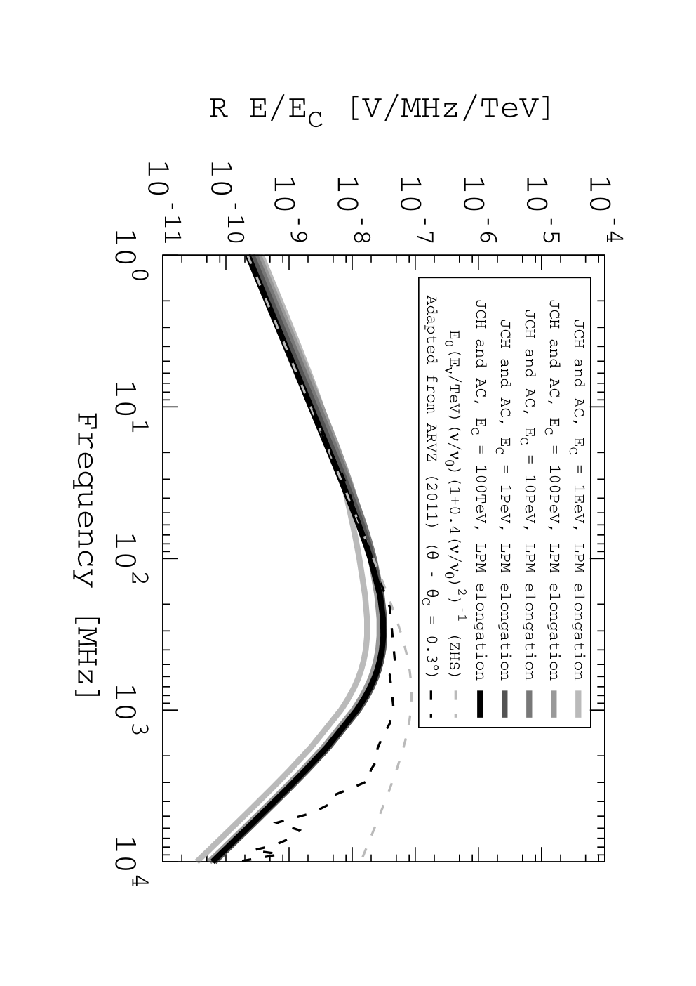
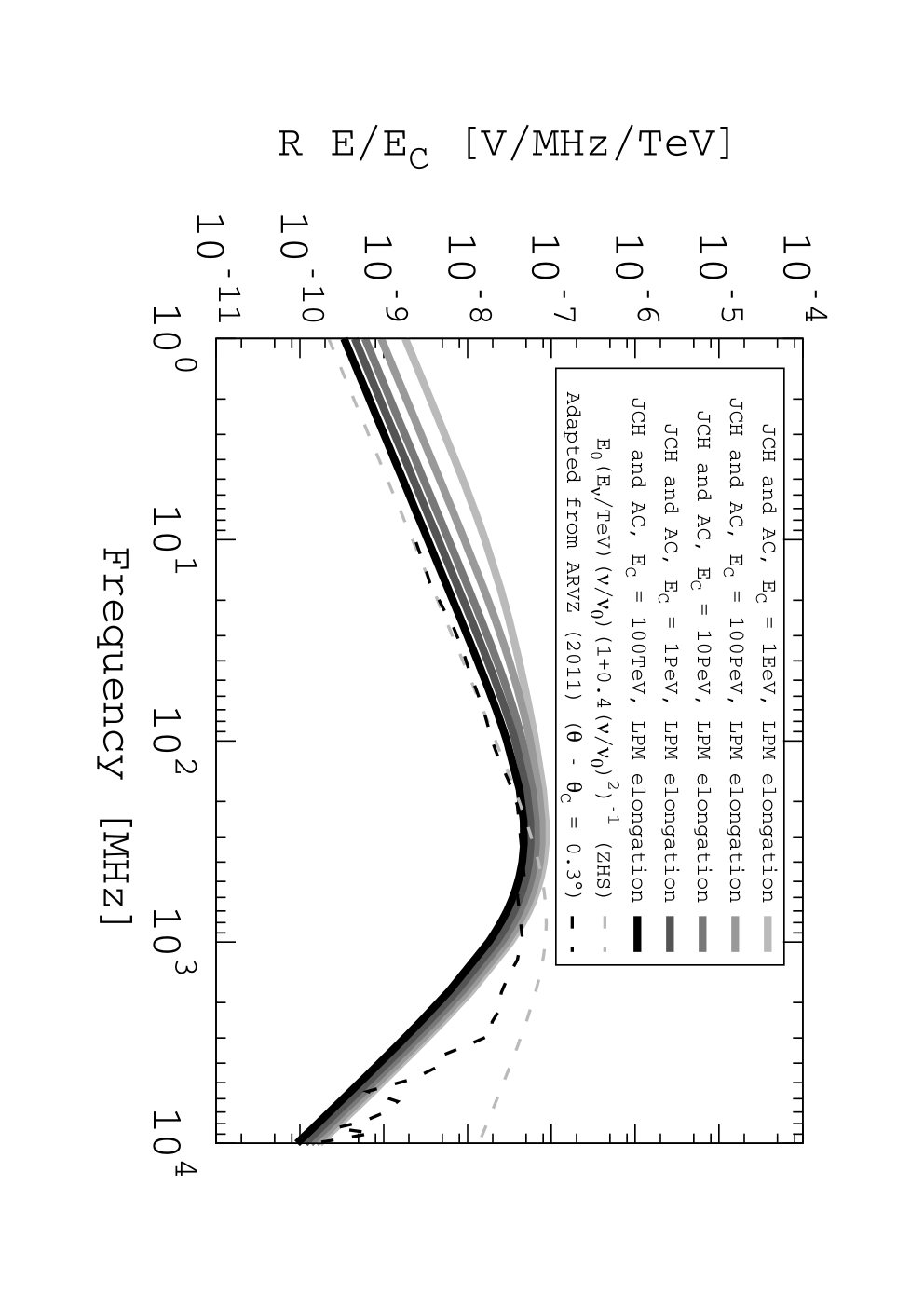
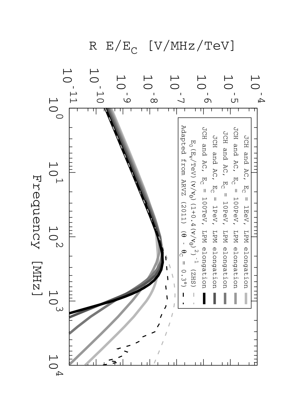
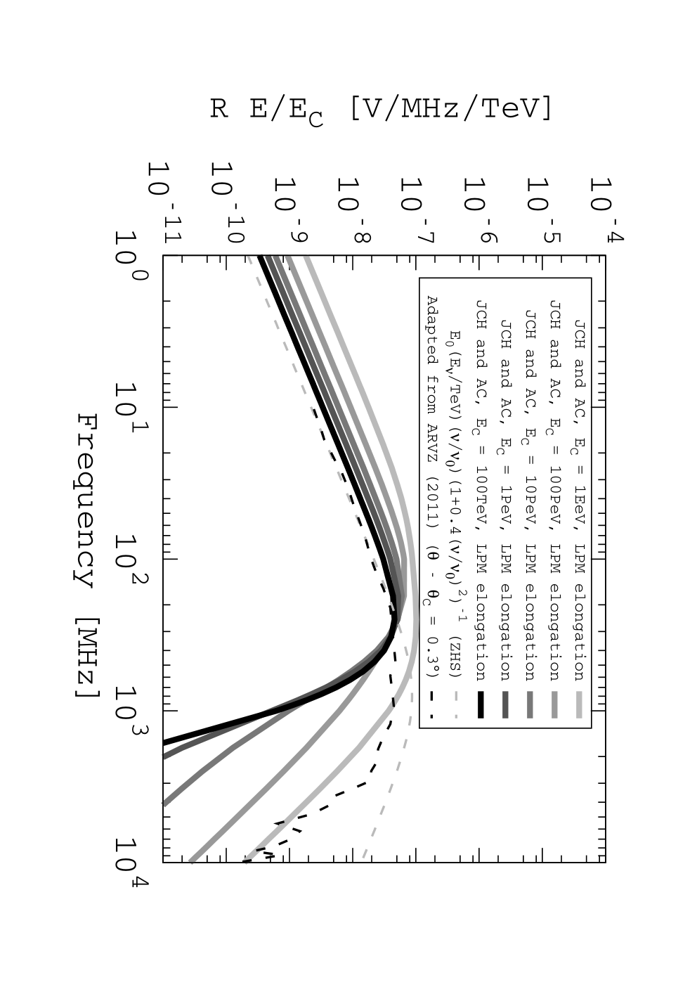
Finally, $|\hat{e}_{\rm\theta}\cdot\mathbf{\widetilde{E}}|$ versus $\theta$ is compared with ZHS and AVZ [PhysRevD.61.023001] in Fig. 8. As with Fig. 7, a counter-intuitive situation arises when $\eta>1$. Similar to the derivation of Eq. 36 from Eq. 13, the angular distribution at fixed frequency is Gaussian in $\Delta\cos\theta=\cos\theta-\cos\theta_{\rm C}$: $|\mathcal{W}(\eta,\theta)|\propto\exp\left(-\frac{1}{2}(\Delta\cos\theta/\sigma_{\rm\Delta\theta})^{2}\right)$, with Cherenkov cone-width

LPM elongation has been applied in Fig. 8, implying that the width of the Cherenkov cone-width should be narrower than ZHS curves. In panel (a), the electromagnetic case agrees with AVZ at 100 MHz ($E_{\rm C}=10$ EeV), but is narrower than ZHS, as expected. The AVZ field for large $|\theta-\theta_{\rm C}|$ corresponds to radiation from sub-dominant peaks in the cascade profile not modelled by RB. The LPM effect is not applied to the hadronic case in the associated code [AlvarezMuniz1998396]. The hadronic case is therefore wider in panel (a), because $\eta<1$ and from Eq. 37, $\sigma_{\rm\Delta\theta}\sim 1/a\nu$. This result follows past far-field approximations in the literature: the Cherenkov-cone is narrower for higher frequencies, and narrower for larger $a$. However, pure hadronic cone-widths from the code should be narrower than AVZ pure hadronic cases, because AVZ do not have the $1/a$ dependence of Eq. 37. In panel (b) ($E_{\rm C}=1$ EeV), the code is compared to a mixed hadronic/electromagnetic cascade from [PhysRevD.61.023001]. AVZ note that pure electromagnetic cascades do not result from electroweak neutrino interactions, because the charged-current case always has a hadronic component. Thus, a linear combination of the solid black and solid gray curves that sum to the black dashed curve will be observed for charged-current interactions. The lower energy in panel (b) relative to panel (a) leads to a wider cone-width because LPM elongation is proportional to $E_{\rm C}$.

In panel (c) of Fig. 8, the same scenario as in panel (a) is depicted, but the frequency is an order of magnitude larger. In panel (d), the same scenario as in panel (b) is depicted, but the frequency is an order of magnitude larger as well. For both scenarios, $\eta\gg 1$, so the Cherenkov cone loses dependence on frequency: $\sigma_{\rm\Delta\theta}\sim\frac{a}{R}\sin^{2}\theta$. This result is that the electromagnetic contribution to the Cherenkov cone is actually wider than the hadronic contribution, because the LPM elongation increases the $a$ of the electromagnetic component, but not the hadronic component. Note that the solid black and solid gray curves do not have to agree with the dashed curves, because they represent different frequencies. The AVZ and ZHS results are identical in all panels, and kept for reference in panels (c) and (d).

Recall from Eq. 10 of Sec. 3.2 that the vector-form of the on-cone field from the RB formalism takes the form:

Let $\hat{E_{\rm 0}}=E_{\rm 0}\sin\theta_{\rm C}\hat{e}_{\theta}$, and define $\omega_{C}$ from $\eta$: $\eta=\omega/\omega_{\rm C}$. Equation 38 may be approximated to first order in the limit $\eta<1$, or $\omega<\omega_{\rm C}$, equivalent to requiring $\lambda R\gtrsim 5a^{2}$. Using the definition of $\eta$, $\nu_{\rm C}=\omega_{\rm C}/(2\pi)$ is

Applying the given limit to Eq. 38, and taking the inverse Fourier transform, yields

The sign convention in the exponential in Eq. 40 is chosen to remain consistent with the RB formalism. The integral may be performed using the Cauchy integral formula, provided that the numerator is analytic ($\exp(-i\omega t_{\rm r})$ obeys the Cauchy-Riemann equations).

Contour integration of Eq. 40 requires a contour $C$ that satisfies Jordan’s lemma and includes all real omega: $\omega\in[-\infty,\infty]$. For the $t_{\rm r}>0$ case, the integral converges along the contour defined by the infinite lower semi-circle because the magnitude of the numerator decreases like $\exp(\operatorname{Im}\{\omega\})$. Note that this is a negatively-oriented contour. For the case $t_{\rm r}<0$, use the fact that $\mathcal{F}_{\omega}(x(-t))=\widetilde{X}(-\omega)$, so $x(-t)=\mathcal{F}_{\omega}^{-1}(\widetilde{X}(-\omega))$, where $\mathcal{F}_{\omega}(x)={\widetilde{X}(\omega)}$ is the Fourier transform of a function $x(t)$. The final solution is piecewise:

MC calculations show the transition at $t_{\rm r}=0$ to be smooth [Eug]. Equation 41 has a characteristic width of $1/\omega_{\rm C}=1/(2\pi\nu_{\rm C})$, implying that the pulse-width is controlled by coherence, in the absence of a form factor. Figure 9 shows $\nu_{\rm C}$ versus the observer distance $R$ and the shower width $a$.

Under the Lorentz gauge condition for Maxwell’s equations, in the absence of static potentials, the negative derivative of the vector potential yields the electric field: $-\partial\textbf{A}/\partial t=\textbf{E}$. Using Eq. 41, the vector potential is

Equation 16 of [PhysRevD.84.103003] is the vector potential at $\theta=\theta_{\rm C}$: