The Arithmetic Geometry of Resonant Rossby Wave TriadsThanks: This research was supported by NSF grant DMS-1401224 and NSF RTG grant 1045119.

Atmospheric Rossby waves are large-scale meanders in high-altitude winds caused by a planet’s rotation. They are a major influence on the weather and have been widely studied. Recently, Petoukhov, Rahmstorf, Petri, and Schellnhuber [24] implicated quasiresonance of Rossby waves in several extreme weather events. Coumou, Lehmann, and Beckmann [9] connected the amplification of Rossby waves with global warming.

Mathematically, Rossby waves are modelled as linear wave solutions to a nonlinear differential equation—the Charney-Hasegawa-Mima equation (CHME) [2]—expressing conservation of potential vorticity (see [23], especially section 3.16). Rossby waves exist in the $\beta$-plane model, in which the Coriolis force varies as a linear function of the latitude (see [23], section 3.17 and chapter 6). The $\beta$-plane model was introduced by Rossby [25], and the CHME was formally derived in the meteorological context by Charney [4, 5]. Many years later, Hasegawa and Mima rediscovered the CHME in a plasma physics context [12, 13]: Rossby waves in the $\beta$-plane model are mathematically equivalent to drift waves in a plasma in a tokamak.

The shape of a Rossby/drift wave is described by its zonal and meridianal wavenumbers, represented as an integer wavevector $(k,\ell)\in\mathbb{Z}^{2}$. The zonal (east/west) wavenumber $k$ is the number of crests per period (around a latitudinal circle), whereas the meridianal (north/south) wavenumber $\ell$ quantifies its meridianal propagation.

Triples of Rossby waves may display resonance, in which case they are called a resonant triad. Under certain physical conditions (large $\beta$), exact resonances dominate the behavior of a system obeying the CHME, by a theorem of Yamada and Yoneda [30].

Enumerating resonant triads up to some large wavenumber bound is a question of practical importance. As Bustamante and Hayat [2] stress in their introduction, information about high-frequency resonances is needed to describe small-scale turbulence in numerical simulations. Moreover, mesoscale waves observed in Jupiter’s atmosphere have wavelenghts of about 20 km, and would have wavenumbers of approximately 20000 if “extended to cover a significant part of Jupiter’s surface” [2]¹¹ 1 See the NASA photo at http://photojournal.jpl.nasa.gov/catalog/PIA00724. Jupiter’s mean radius $r$ is about 70000 km, and the waves were observed propagating east-west at $15^{\circ}$ South. So, the zonal wavenumber would be $2\pi r\cos\left(15^{\circ}\right)/(20{\rm\ km})\approx 20000$ waves per period (or about 3000 waves per radian)..

The set of resonant triads may be described as the set of integer solutions to a Diophantine equation, as explained in the next section. In this paper, we give two descriptions of the solutions to this equation: a rational parametrization and an elliptic fibration.

The Charney-Hasegawa-Mima equation is²² 2 Sometimes an additional term $U\frac{\partial}{\partial x}\left(\Delta\psi\right)$ for a mean zonal flow is included; including it would have no effect on the Diophantine equation we’ll obtain for resonant wavevectors.

where $\psi=\psi(x,y,t)$ is a function on $\mathbb{R}^{2}\times\mathbb{R}$. This first two terms are linear, and their sum is called the linear part. The last term is nonlinear. Standard notation is used for the Euclidean Laplacian and the Poisson bracket:

and $\beta>0$ and $F\geq 0$ are constants.³³ 3 For atmospheric Rossby waves, $\beta=\frac{2\varpi\cos\theta}{r}$, where $\varpi$ is the planet’s angular rotation, $\theta$ is the latitude, and $r$ is the planet’s mean radius. The constant $F=\frac{1}{R^{2}}$, where $R$ is the Rossby deformation radius. The physical meanings of the parameters are: $(x,y)$ are spacial coordinates, $t$ is a temporal coordinate, and $\psi$ the streamfunction of an incompressible flow.

For the derivation of the CHME in both the meteorology and plasma physics contexts, see [11].

We will only consider the limiting case of (1.1) to infinite Rossby deformation radius. Equivalently, we set $F=0$. So, the equation we will consider is

The equation (1.4) has a rich set of solutions, and no general solution is known. However, one simple family of solutions, called Rossby waves, are given by exponential functions.⁴⁴ 4 The real part of $\psi_{k,\ell}$ is also a solution, and, in some applications, may instead be called a Rossby wave.

Indeed, Rossby waves satisfy both the linear and nonlinear parts of (1.4), separately. The vector $(k,\ell)\in\mathbb{R}^{2}$ is called the wavevector, $k$ is the zonal wavenumber, and $\ell$ is the meridional wavenumber.

Generally, linear combinations of Rossby waves no longer satisfy the nonlinear part of the CHME. However, under certain conditions, triads $\{(k_{1},\ell_{1}),(k_{2},\ell_{2}),(k_{3},\ell_{3})\}$ of Rossby waves “resonate” so that the real part of a certain linear combination

where $\tau$ is a slow time scale, satisfies the CHME. See [17] and especially the supplement [18] for details, and [23, 22, 10] for additional background.

Resonant triads of Rossby waves satisfy the conditions

We have $(k_{2},\ell_{2})=(k_{3}-k_{1},\ell_{3}-\ell_{1})$, so the condition for $\{(k_{1},\ell_{1}),(k_{2},\ell_{2}),(k_{3},\ell_{3})\}$ to be a resonant triad comes down to the condition on the angular frequencies:

which we rewrite as

We impose the additional requirement that the solutions to the CHME are periodic in both spatial coordinates:

Equivalently, rather than considering the CHME on $\mathbb{R}^{2}\times\mathbb{R}$, we can specify that the domain is $\left(\mathbb{R}/2\pi\mathbb{Z}\right)^{2}\times\mathbb{R}$. Periodicity implies that the wavenumbers are integers.

Several authors framed the problem of enumerating resonant triads as a number-theoretic question [2, 15]. For convenience, change notation and set $(k_{1},\ell_{1},k_{3},\ell_{3})=(a,b,x,y)$.

Bustamante and Hayat [2] classify integer solutions to (1.15) by mapping them bijectively to representations of zero by a certain quadratic form, yielding an algorithm for enumerating all resonant triads (see further discussion in section 1.8). Kishimoto and Yoneda [15] show that there are no solutions where $b=0$. Both sets of authors also draw attention to a special family of resonant triads (called “pure cube triads” by [2]):

where $s,t\in\mathbb{Z}$.

Other objects of interest to [15] and [30] are the wavevector set $\Lambda$ and primitive wavevector set $\Lambda^{\prime}$, and their distribution within the integer lattice.

The condition $ax(a-x)\neq 0$ imposed in (1.19–1.20) rules out single wave solutions and zonal resonances (see also the discussion at the end of section 3.1).

The left hand side of (1.15) is a homogeneous rational function in $(a,b,x,y)$, so any rational solution $(a_{0},b_{0},x_{0},y_{0})$ gives rise to a primitive integer solution $(\lambda a_{0},\lambda b_{0},\lambda x_{0},\lambda y_{0})$ by clearing denominators and dividing out common factors. A primitive integer solution is one where $\gcd(a,b,x,y)=1$, and any integer solution is an integer multiple of a primitive integer solution. The problem of enumerating primitive integer solutions to (1.15) is the same as the problem of enumerating rational solutions up to a common factor, that is, rational solutions in projective space.

We may clear denominators in (1.15) and do some algebra to obtain the equation

We consider (1.15) and (1.21) as equations in projective space $\mathbb{P}^{3}$ with homogeneous coordinates $[a:b:x:y]$. Let $X$ be the locus of solutions to (1.21) in $\mathbb{P}^{3}$; $X$ is a degree $5$ surface. Let $X^{\circ}\subset X$ be the locus of solutions to (1.15).

Finding points on $X$ is essentially the same problem as finding points on $X^{\circ}$; $X$ has a few extra points that are easy to describe (see section 2.1).

For fixed $(a,b)\in\mathbb{C}^{2}\setminus(0,0)$, let $C(a,b)$ be the locus of (1.21) in affine space $\mathbb{A}^{2}$. Over any field containing $a$ and $b$, $C(a,b)\cong C(\lambda a,\lambda b)$ by $(x,y)\mapsto(\lambda x,\lambda y)$, so we think of $C(a,b)$ as depending only on $[a:b]\in\mathbb{P}^{1}$. However, we will also want to consider, for $(a,b)\in\mathbb{Z}^{2}$, the integer points on $C(a,b)$, and a scaling factor may enlarge the set of integer points.

We show that $X$ is a rational surface, that is, a surface with a rational parametrization (meaning, a birational isomorphism with $\mathbb{P}^{2}$ defined over $\mathbb{Q}$). We give the following parametrization, which may be used to directly enumerate integer points on $X$.

The surface $X$ may be described more precisely as a rational elliptic surface,⁵⁵ 5 The definition of an elliptic surface is usually taken to include the conditions that the surface is smooth and the generic fiber is smooth. We do not assume either of these conditions; indeed, $X$ is non-smooth and $C(a,b)$ is always non-smooth. that is, a surface with a map $X\to\mathbb{P}^{1}$ so whose generic fiber has geometric genus 1, along with an identity section $\mathbb{P}^{1}\to X$. The integer points $(x,y)$ on a fiber $C(a,b)$ are the wavenumbers that exhibit resonance with $(a,b)$.

The rational points on an elliptic curve have the structure of a finitely generated abelian group, the Mordell-Weil group. We prove a result about the structure of this group for $C(a,b)$.

A “typical” elliptic curve over $\mathbb{Q}(t)$ has trivial Mordell-Weil group, that is, rank 0 and no torsion. Thus, Theorem 1.4 says that $X$ is a special member of the class of elliptic surfaces.

For definitions and background information about elliptic curves and elliptic surfaces, see Silverman’s books [27, 28].

This paper describes the surface $X$ in two different ways. The first description is a parametrization of $X$ as a rational surface. This parametrization gives a procedure for enumerating points on $X$ (i.e., primitive resonant Rossby triads). The algorithmic performance of this enumeration procedure is discussed in the next section.

The second description is a fiberwise description: It describes all the triads with $a/b$ fixed. For example, the resonant wavevectors with $a/b=1$---that is, those whose wave packets propagate due northward⁶⁶ 6 The group velocity of $\psi_{a,b}$ is $C_{g}:=\frac{\partial\omega}{\partial a}=\left(\frac{\beta\left(a^{2}-b^{2}\right)}{\left(a^{2}+b^{2}\right)^{2}},\frac{2\beta ab}{\left(a^{2}+b^{2}\right)^{2}}\right)$, so when $a/b=1$, the zonal component is zero and the meridional component is positive.—are the rational points on $C(1,1)$, a rank 1 elliptic curve. This special case is discussed further in section 4.

Our parametrization of $X$ generalizes the family of points 1.16 by introducing a third variable, $u$. Like Bustamante and Hayat’s classification (which involves a different rational change of variables), our parametrization provides a conjecturally fast procedure for enumerating points on $X$. Computational issues are discussed in 1.8.

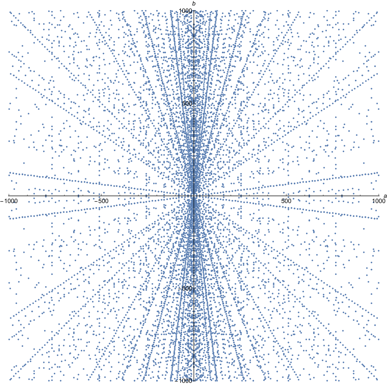
Our fiberwise description of $X$ is new and yields new information about the primitive wavevector set, shown in Figure 2. Specifically, the nonzero rank of $C(a,b)$ implies that there are infinitely many points on any line through the origin with rational slope. In other words, for any nonzero rational number $r$, there are infinitely many primitive resonant wavevectors $(x,y)\in\Lambda^{\prime}$ such that $\frac{x}{y}=r$. Equivalently, there are infinitely many primitive resonant wavevectors with any southward phase direction of rational slope.

Kishimoto and Yoneda [15] remark that the wavenumber set appears highly anisotropic. Specifically, this set becomes sparser faster as $a\to\infty$ than as $b\to\infty$. Based on numerical observations, we suggest some stronger conjectures about the anisotropy.

Numerical evidence suggests that the horizontal lines contain only finitely many points in the wavenumber set.

On the other hand, it’s easy to produce infinitely many points on some vertical lines: For example, if $a=s^{4}$, then $(a,st^{3})\in\Lambda$ for any $t\in\mathbb{Z}$. We conjecture, based on numerical computations, that there are actually infinitely many points on any vertical line (except the $b$-axis) in Figures 1 and 2.

Finally, we make a remark about the distribution of ranks of these elliptic curves. For $(a,b)\in[1,100]^{2}$, we found (using Magma) that 39% of the $C(a,b)$ had rank 1, 46% had rank 2, 13% had rank 3, and 1% had rank 4. This looks similar to numerical data number theorists have obtained for other rank 1 families. However, the widely believed Minimalist Conjecture predicts that, in the limit as $N\to\infty$, 50% of the $C(a,b)$ in $[1,N]^{2}$ should have rank 1, and 50% rank 2. See [1] for background about this problem and extensive numerical computations.

Bustamante and Hayat’s classification [2] yields an algorithm for enumerating the set of nontrivial resonant triads. They identifying this set with the zero-set of a diagonal quadratic form in four variables, and enumerate that zero-set using classical theorems on representations of integers as $n=x^{2}+dy^{2}$ for $d=1,3$. Bustamante and Hayat pose the challenge of generating all or most primitive triads within a box of size $N$:

For $N=5000$, Bustamante and Hayat’s method produced $870\times 12=435\times 24$ triads in 20 minutes in Mathematica on an “8-core desktop” [2]. Bustamante and Hayat compare this to a naïve search, which would take about 15 years to complete, although Kartashova and Kartashova [14] remark that a smart search (confined to an open neighborhood of $X$) would be faster.⁷⁷ 7 Kartashova and Kartashova describe, in section IV of [14], a search algorithm enumerating $B_{N}$ in $O(N^{3})$ time, compared to $O(N^{4})$ for a naïve search.

For our method, we use the parametrization (1.2) to enumerate points on $X$, with a slight modification. We changed coordinates on $\mathbb{P}^{2}$ to make it easier to mod out by symmetries: We set $w=s-2u$ and use the coordinates $[s:t:w]$. Then all nontrivial resonant triads are generated by $s>0$, $t>0$, $w>0$, $t^{2}>\frac{1}{4}(3s-w)(s+w)$, and by the action of the group of order 24 generated by the symmetries

Searching $0<s,t,w\leq 200$ and applying symmetries took about 5 minutes of CPU time and found $443\times 24$ triads in $B_{5000}$. Searching $0<s,t,w\leq 500$ and applying symmetries took about 80 minutes and found $463\times 24$ triads in $B_{5000}$. Computations were performed in Mathematica on a MacBook Pro laptop (2.9 GHz dual-core i7).

We have not established any upper bound on the search space necessary to output all nontrivial resonant triads up to a given wavenumber bound. We hope to establish such a bound in a future paper.

Our object is to determine the rational points of $X^{\circ}$—that is, the primitive Rossby wave triads. It’s convenient to study the Zariski closure $X$, which will have a few extra points. Before we do so, it’s important to quantify the difference between these two sets. We also need to understand the singular points of $X$, because the birational map from $X\to\mathbb{P}^{2}$ we will define in section 2.2 will be undefined at these points (and well-defined everywhere else).

The real points of $X\setminus X^{\circ}$ correspond to “resonant triads” that are actually just single Rossby waves. If, for example, $x-a=y-b=0$, then the triad is $\{(a,b),(0,0),(a,b)\}$, and the conditions on the $A_{i}(t)$ (see equation (5) in [18]) reduce to $A_{1}^{\prime}(t)=A_{3}^{\prime}(t)=0$. Thus, 1.7 becomes $\psi=\Re\left(C\psi_{a,b}\right)$, the real part of a single Rossby wave.

Note that $X^{\rm sing}$ is contained in $X\setminus X^{\circ}$; that is, $X^{\circ}$ is everywhere smooth.

We will now prove Theorem 1.2, which we restate here for convenience.

We normalize the $C(a,b)$ to obtain a smooth model, and convert to Weierstrass form.

We are now ready to prove Theorem 1.3, which we restate here for convenience.

References

- [1] J. S. Balakrishnan, W. Ho, N. Kaplan, S. Spicer, W. Stein, and J. Weigandt, Databases of elliptic curves ordered by height and distributions of Selmer groups and ranks, arXiv preprint arXiv:1602.01894, (2016).
- [2] M. D. Bustamante and U. Hayat, Complete classification of discrete resonant Rossby/drift wave triads on periodic domains, Commun. Nonlinear Sci. Numer. Simul., 18 (2013), pp. 2402–2419.
- [3] C. Chabauty, Sur les points rationnels des courbes algébriques de genre supérieur à l’unité, C. R. Acad. Sci. Paris, 212 (1941), pp. 882–885.
- [4] J. G. Charney, The dynamics of long waves in a baroclinic westerly current, Journal of Meteorology, 4 (1947), pp. 136–162.
- [5] , On the scale of atmospheric motions, Geofys. Publ., 17 (1948), pp. 3–17.
- [6] R. F. Coleman, Effective Chabauty, Duke Math. J., 52 (1985), pp. 765–770.
- [7] , Torsion points on curves and -adic abelian integrals, Ann. of Math. (2), 121 (1985), pp. 111–168.
- [8] Computational Algebra Group, Magma handbook, Sydney, 2015.
- [9] D. Coumou, J. Lehmann, and J. Beckmann, The weakening summer circulation in the northern hemisphere mid-latitudes, Science, 348 (2015), pp. 324–327.
- [10] A. D. D. Craik, Wave Interactions and Fluid Flows, Cambridge University Press, 1988.
- [11] A. Hasegawa, C. G. Maclennan, and Y. Kodama, Nonlinear behavior and turbulence spectra of drift waves and Rossby waves, Physics of Fluids (1958-1988), 22 (1979), pp. 2122–2129.
- [12] A. Hasegawa and K. Mima, Stationary spectrum of strong turbulence in magnetized nonuniform plasma, Physical Review Letters, 39 (1977), p. 205.
- [13] , Pseudo-three-dimensional turbulence in magnetized nonuniform plasma, Physics of Fluids (1958-1988), 21 (1978), pp. 87–92.
- [14] A. Kartashov and E. Kartashova, Discrete exact and quasi-resonances of rossby/drift waves on -plane with periodic boundary conditions, arXiv preprint arXiv:1307.8272, (2013).
- [15] N. Kishimoto and T. Yoneda, A number theoretical observation of a resonant interaction of rossby waves, arXiv preprint arXiv:1409.1031, (2014).
- [16] S. Lang, Elliptic Curves: Diophantine Analysis, Springer, 1978.
- [17] P. Lynch, Resonant Rossby wave triads and the swinging spring, Bulletin of the American Meteorological Society, 84 (2003), pp. 605–616.
- [18] , Supplement to Resonant Rossby wave triads and the swinging spring, Bulletin of the American Meteorological Society, 84 (2003), pp. 616–616.
- [19] B. Mazur, Modular curves and the Eisenstein ideal, Inst. Hautes Études Sci. Publ. Math., 47 (1977), pp. 33–186 (1978).
- [20] , Rational isogenies of prime degree (with an appendix by D. Goldfeld), Invent. Math., 44 (1978), pp. 129–162.
- [21] W. McCallum and B. Poonen, The method of Chabauty and Coleman, in Explicit methods in number theory, vol. 36 of Panor. Synthèses, Soc. Math. France, Paris, 2012, pp. 99–117.
- [22] A. H. Nayfeh, Perturbation Methods, John Wiley & Sons, 2008.
- [23] J. Pedlosky, Geophysical Fluid Dynamics, Springer Science & Business Media, 2013.
- [24] V. Petoukhov, S. Rahmstorf, S. Petri, and H. J. Schellnhuber, Quasiresonant amplification of planetary waves and recent northern hemisphere weather extremes, Proceedings of the National Academy of Sciences, 110 (2013), pp. 5336–5341.
- [25] C.-G. Rossby et al., Relation between variations in the intensity of the zonal circulation of the atmosphere and the displacements of the semi-permanent centers of action, Journal of Marine Research, 2 (1939), pp. 38–55.
- [26] R. Schoof, Elliptic curves over finite fields and the computation of square roots mod , Mathematics of computation, 44 (1985), pp. 483–494.
- [27] J. H. Silverman, The Arithmetic of Elliptic Curves, vol. 106 of Graduate Texts in Mathematics, Springer-Verlag, New York, 1986.
- [28] , Advanced Topics in the Arithmetic of Elliptic Curves, vol. 151 of Graduate Texts in Mathematics, Springer-Verlag, New York, 1994.
- [29] M. Stoll, Rational points on curves, J. Théor. Nombres Bordeaux, 23 (2011), pp. 257–277.
- [30] M. Yamada and T. Yoneda, Resonant interaction of Rossby waves in two-dimensional flow on a plane, Phys. D, 245 (2013), pp. 1–7.