∎
Driven interfaces: from flow to creep through model reduction
Abstract
The response of spatially extended systems to a force leading their steady state out of equilibrium is strongly affected by the presence of disorder. We focus on the mean velocity induced by a constant force applied on one-dimensional interfaces. In the absence of disorder, the velocity is linear in the force. In the presence of disorder, it is widely admitted, as well as experimentally and numerically verified, that the velocity presents a stretched exponential dependence in the force (the so-called ‘creep law’), which is out of reach of linear response, or more generically of direct perturbative expansions at small force. In dimension one, there is no exact analytical derivation of such a law, even from a theoretical physical point of view. We propose an effective model with two degrees of freedom, constructed from the full spatially extended model, that captures many aspects of the creep phenomenology. It provides a justification of the creep law form of the velocity-force characteristics, in a quasistatic approximation. It allows, moreover, to capture the non-trivial effects of short-range correlations in the disorder, which govern the low-temperature asymptotics. It enables us to establish a phase diagram where the creep law manifests itself in the vicinity of the origin in the force – system-size – temperature coordinates. Conjointly, we characterise the crossover between the creep regime and a linear-response regime that arises due to finite system size.
Keywords:
Disordered systems Non-equilibrium dynamics Creep law Non-linear response Kardar–Parisi–Zhang universality class1 Introduction
Disorder can radically affect the behaviour of physical phenomena. An archetypal class of systems is given by extended elastic objects (lines or manifolds) which fluctuate in an heterogeneous medium [1]. Examples range from interfaces in magnetic or ferroic [2] materials, vortices in superconductors [3] to solid membranes in chemical or biological liquids, and fronts in liquid crystals [4, 5]. In the absence of disorder, the geometry and dynamical properties of such systems are in general resulting from a simple interplay between elastic constraints and thermal noise. The addition of disorder (impurities, quenched inhomogeneities, space-time noise) can alter the geometry of the interface, by changing it from flat to rough, or by modifying its fractal dimension in scale-invariant systems [6]. For models in the Kardar-Parisi-Zhang class (KPZ) class [7] the disorder transforms the diffusive spatial fluctuations of a line into superdiffusive ones (see [8, 9, 10, 11, 12] for reviews).
We are interested in the non-equilibrium motion induced by an external drive applied to such systems with quenched disorder. In the disorder-free situation, Ohm’s linear law [13] between the observed average velocity and the applied force yields a simple linear response. In the presence of disorder, the situation is more complex; the so-called ‘creep law’ is an example of velocity-force characteristics for which linear response does not hold, even in the very small force limit. It is described by a stretched-exponential velocity-force relation of the form (where we set scaling parameters to 1) depending on the creep exponent , which is non-analytic at zero force . It was derived in the context of dislocations in disordered media [14, 15] and motion of vortex lines [16, 17, 18], and gave rise to a number of studies, ranging from the initial scaling and renormalization-group (RG) analysis [7, 19], to equilibrium [20] and non-equilibrium functional renormalization group (FRG) studies [21, 22], and, in the picture of successive activation events, to the study of the distribution of energy barriers [23] and of activation times [24, 25]. Numerical studies confirm its validity for one-dimensional interfaces [26, 27, 28, 29] (see [30] for a review), and experimental results for driven domain walls in ultrathin magnetic layers [31] are compatible with a stretched exponential velocity-force relation with a creep exponent .
Several questions yet remain to be clarified. The first class of questions pertains to the derivation of the law itself: RG analysis in dimension one is known to be non-convergent, and FRG approaches are valid perturbatively in dimension far from dimension (). Different power-counting scaling arguments lead to different values of the creep exponent (as we detail in subsection 2.4). The second class of questions is related to the understanding of the finite-size regime: one indeed expects that for a finite system, the linear response should be valid at very low forces; this rises the question of how to depict the crossover between this linear regime and the creep law. More generically, we aim at constructing a phase diagram in the three coordinates (force, inverse of system size, temperature) provided by the parameters of interest, which would depict criticality around its origin and specify the characteristic scales of the creep regime.
In this article, we construct an effective model describing the motion of the driven interface at fixed lengthscale. It allows us to recover the creep law and to extend the description of the dynamics from low forces to larger forces, and to characterise the crossover between creep and linear response in finite systems in the very small force regime. Previous approaches have dealt with ‘zero-dimensional’ toy models where a particle with one degree of freedom moves in a one-dimensional random potential [25, 32, 33]. However, the distribution of such a random potential that would summarise the effect of the disorder experienced by the full segment of the interface would prove very delicate to describe in our system of interest. Indeed, an important issue of driven systems with one degree of freedom is that very large barriers always block the motion, making the extreme statistics of the disorder play an essential role. In contrast, the cost of the elastic deformations allowed in higher dimensions allows to counterbalance large inhomogeneities in the environment: deep wells in the disorder potential cannot pin the interface beyond the (unbounded) energetic cost of the elastic deformations that they would impose as the interface moves — thus rendering the dynamics of the system less sensitive to the extremes of the disorder distribution. The effective model that we propose has two degrees of freedom which allow to capture in a minimalist way such competition between elasticity and disorder.

We now summarise our findings, before providing their derivation in the next sections. We establish a phase diagram in the force – system-size – temperature coordinates (see Fig. 1) that describes the regimes where the velocity-force dependence is of the creep type or of the flow type. The creep law itself appears in the critical region of the diagram, in the low-force, low-temperature and large-system size regime. Physically, the creep regime holds in regions where a specific form of scale invariance holds (relevant observables scaling simply with all parameters), while the flow regime appears whenever the system-size is too small for such scaling to hold. Our results complement previous numerical and phenomenological studies on the scalings of the driven interface [29, 30, 34]: we are able to analyse the role of finite system size (complementing [35]), but we cannot probe the depinning regime that was examined in those studies, which is out of reach of our effective model reduction. The novelty of our approach lies also in the methodology that we propose, which provides a well-defined procedure, solving in particular a power-counting dilemma for the scaling arguments: we device an effective model for the driven interface at fixed scale and propose saddle-point point argument at small forces which justifies why only one out of two possible power-counting arguments (either on the Hamiltonian or on the free energy) yields the correct creep exponent. We detail how a mean first passage time (MFPT) description allows to handle non-equilibrium issues within an equilibrium settings. Then, from the combination of those tools, we are able to extend the creep law and we describe the crossover from the finite-system size very small velocity regime to the creep law. Most importantly, we take into account the role of finite disorder correlations at short-range [11, 36, 37, 38, 39] which are essential to understand the low-temperature asymptotics, and in particular to identify the characteristic energy and characteristic force of the creep law.
The article is organised as follows: we precise the model and known results in Sec. 2. We review the particle toy-model (with one degree of freedom) in Sec. 3 as it serves as a basis to our analysis. In Sec. 4, we describe the effective model with two degrees of freedom and explain how it provides a useful framework to understand the creep law. In Sec. 5, we use this description to analyse the crossover from creep to linear response at small forces in finite systems. We finally discuss our results in Sec. 6 and present perspectives in Sec. 7. Our exposition is self-contained; the reader familiar with the subject can read in Sec. 2.3 the definition of the tilted KPZ problem and directly jump to Sec. 4 for the analysis the effective model derived from it. Table 1 summarises the notations.
| Variable | Signification | Expression | Eq./Fig./§ | |
| Coordinates | Transverse coordinate | |||
| Longitudinal coordinate | ||||
| Physical time | Fig. 2 | |||
| Interface segment length | ||||
| Starting and arrival points | ||||
| Model | Elastic constant | (1) | ||
| parameters | Disorder strength | (2) | ||
| Temperature | § 2.1 | |||
| Disorder correlation length | (2) | |||
| Driving force | (1) | |||
| Friction coefficient | (1) | |||
| Total interface length | § 5.1 | |||
| Thermodynamic | Partition function | (15) | ||
| quantities | Free energy | (16) | ||
| Disorder free energy | (36) | |||
| Observables | Steady-state velocity | (52), (59) | ||
| Mean First Passage Time | (38), (50-51) | |||
| Effective | Effective friction | (35) | ||
| parameters | Effective temperature | (35) | ||
| Characteristic | Characteristic temperature | (43) | ||
| parameters | Larkin length (at low ) | (61) | ||
| Characteristic force | (53) | |||
| Characteristic barrier | (53),(70) | |||
| Critical depinning force | Fig. 2 | |||
| Finite- | Disorder free-energy strength | (42-43),(64) | ||
| parameters | Fudging parameter | solution of (66) | (66) | |
| Optimal length | (54) | |||
| -dependent Larkin length | (63) | |||
| Max. force until | (55) | |||
| Max. force until | (68) | |||
| Fudging exponent | (66) |
2 Model and questions
We present in this section the model of one-dimensional (1D) interface that we consider, recalling its known phenomenology in Sec. 2.1. We describe the correspondence, in the non-driven case, between the equilibrium distribution of the position of the interface and the directed polymer in Sec. 2.2, motivated by understanding the fluctuations of the interface at fixed length — a crucial step for our scaling analysis and that has a natural formulation in the directed polymer language. We then construct in Sec. 2.3 a variation of the equilibrium problem in which the interface is subjected to a tilted random potential but also to boundary conditions forbidding the development of a non-zero velocity state, and that we will use as a starting point in our approach in the following sections. Finally, to motivate our study, we compare in Sec. 2.4 different power-counting arguments presented in the literature either at the Hamiltonian or at the free-energy level, which do not lead to the same result and call for a detailed analysis.
2.1 Dynamics
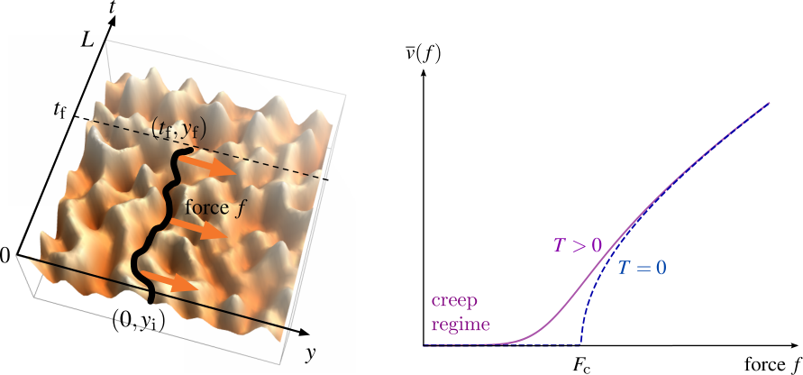
We denote by the (physical) time of the interface and introduce as described in Fig. 2 a -dependent position of the interface, of longitudinal coordinate . Its evolution is described by the overdamped Langevin equation
| (1) |
where is the elastic constant, the friction coefficient and the driving force. Thermal fluctuations at temperature are described by the centred white noise of correlations . We have set Boltzmann’s constant to . The disorder has a Gaussian distribution of zero mean and correlations fully described by its two-point function
| (2) |
Longitudinal correlations in the direction are absent while transverse correlations are described by a function scaling as and normalised as . More specifically, the correlator is a “smooth delta” describing short-range correlations at scale , that tends to a Dirac delta as goes to zero. The strength of disorder is described by the parameter . Such type of quenched disorder belongs to the ‘random bond’ class.
The driving force induces a motion of the interface, characterised by its mean velocity . The linear response fails for an infinite interface even in the small-force regime, and instead of a velocity proportional to one observes the ‘creep law’
| (3) |
This is the stretched exponential behaviour, already mentioned in the introduction, of creep exponent , characteristic energy scale and characteristic force . It is valid in the regime of low forces compared to the depinning critical force and of low temperatures compared to the effective barrier (see Fig. 2, Right). The characteristic parameters and are usually identified numerically or by a fitting procedure; in this article, we derive an expression of and in terms of the model parameters , , valid in the low-temperature limit of the 1D interface (see Sec. 4.3), including a non-trivial temperature dependence. The behaviour (3) has been verified experimentally for interfaces in magnetic materials on several decades of velocities [31] and tested numerically with success [27, 28, 29, 30]. It was originally predicted in other dimensionalities in the description of the motion of vortices in random materials (modelling for instance vortices in type-II superconductors), using either scaling [14, 18] or perturbative FRG arguments in an expansion around spatial dimension 4, first used within an equilibrium frame [20] and then extended out of equilibrium [21].
2.2 Zero driving force: correspondence with the directed polymer
We first consider the equilibrium case at zero driving force , which has been extensively studied (see [9, 10, 11] for reviews). The Langevin equation becomes
| (4) |
At fixed disorder , the system eventually reaches an equilibrium steady state in the long-time limit: the non-normalised weight of a segment of interface of length is , where the Hamiltonian reads
| (5) |
where the boundaries of the integral are determined by the domain of definition of . The Boltzmann equilibrium form of this steady state can directly be read from the equation of evolution (4) that one can rewrite as
| (6) |
allowing to recognise an overdamped Langevin dynamics of force term deriving from the Hamiltonian (5). One can explicitly check from the functional Fokker-Planck equation associated to (4):
| (7) |
that the distribution
| (8) |
is a zero-probability-current steady-state solution (hence an equilibrium one)
| (9) |
Spatial boundary conditions then determine how the Boltzmann weight comes into play when defining probability distributions; a well-understood situation is that of the continuous directed polymer, where the interface is attached at its extremities in and (adopting so-called point-to-point configurations, see Fig. 2, left). The equilibrium weight at temperature of realisations of the interface starting from and arriving in in a random potential is the weight defined by the path integral:
| (10) |
For instance, at fixed length and fixed initial position , the probability density of interfaces arriving in is . The statistical properties of the ‘partition function’ (10) have been the subject of extensive studies, as the continuous directed polymer belongs to the Kardar-Parisi-Zhang (KPZ) [7] universality class of models (see [8, 9, 10, 11, 12] for reviews). A noticeable fact is that the directed polymer free energy
| (11) |
verifies the KPZ equation [19] with sharp-wedge initial condition: denoting for short one has
| (12) |
We will present and/or derive its useful symmetries for our study when needed (see Appendix A and also Ref. [40] for a systematic study of KPZ symmetries). Note that a proper mathematical definition of (10) as an expectation over Brownian bridges [41] and the passage to the KPZ equation (12) through the application of Itō’s lemma requires the appropriate removal of -diverging constants (see [42] for a pedagogical introduction).
2.3 The tilted directed polymer: equilibrium at non-zero
The original dynamics of the driven interface (1) at non-zero driving force can also be rewritten in a form similar to (6)
| (13) |
as an overdamped Langevin equation with forces deriving from a tilted Hamiltonian
| (14) |
One can still write a Boltzmann equilibrium distribution which is a zero-probability-current solution to the steady-state functional Fokker-Planck equation, similarly to what we observed in (9) (with ). However, it describes the steady state of the system only in situations where the dynamics is reversible.In the presence of the drive , such an equilibrium can only be reached with appropriate spatial boundary conditions, for instance for a (half-)bounded system with one wall ( for , for ) or two walls ().
Such boundary conditions block the motion of the interface and make average velocity equal to zero ; consequently, in the large time limit, they cannot depict the steady state of the non-equilibrium driven interface. However, as we will argue in Sec. 4, the distribution of point-to-point interfaces in this equilibrium settings still provides an effective model for the non-equilibrium quasistatic motion of the driven interface. To construct this effective model, the central quantity that we will use is the weight of a trajectory starting from and arriving in in a tilted random potential :
| (15) |
The path integral is performed over the interface configurations respecting the equilibrium boundary conditions with one or two walls. Similarly to (11) we define a tilted free energy
| (16) |
in which one can precisely identify the contributions scaling differently from each other, as we detail in 4.2.
2.4 Issues occurring when scaling the Hamiltonian
Before describing the symmetries of the above introduced models, we discuss the scaling arguments based on the Hamiltonian (14) that are usually put forward to derive the creep law in an formal way, and how they can present an inconsistency. In standard heuristic arguments on the scaling properties of the Hamiltonian (see [28] for a review), it is assumed that the fluctuations of a segment of length of the interface scale according to with the roughness exponent of the interface. Accordingly, the elastic, disorder and driving contributions to the tilted Hamiltonian (14) scale respectively as
| (17) | ||||
| (18) | ||||
| (19) |
where for the disorder contribution (18) one uses (the symbol meaning that the scaling holds in distribution). Matching the elastic and driving contributions (17) and (19) gives the scaling of the optimal interface length displaced at a force
| (20) |
In this argument, it is then asserted that the average velocity scales as the inverse of the Arrhenius time to cross an energetic barrier, itself scaling as one of the contributions (17-19) to the Hamiltonian. Using either or yields by definition of the same result
| (21) |
This expression of the creep exponent matches for the generic result known in dimension : (see [28] for a review). Substituting the KPZ roughness exponent , one finally obtains the expected creep exponent .
Nevertheless, this power-counting procedure lacks a proper justification, and in fact presents an inconsistency. The roughness exponent that it would imply is incorrect; indeed, matching the elastic and disorder contributions (17) and (18) yields hence . This is the so-called Flory exponent of the Hamiltonian, different from the exact value which characterises the geometrical fluctuation of the 1D interface at large scales. Besides, even if one decides to impose the value and that one tries to find by matching the disorder contribution (18) (instead of the elastic one) to the driving contributions (19), one gets
| (22) |
which would yield incorrectly and .
At , for the determination of the roughness exponent , the origin of that problem has been elucidated in Ref. [11]: in fact one cannot assume that typically scales with the same exponent at all lengthscales, as was done in (17-19). This is seen for instance by the result that the roughness function , which describes the variance of the endpoint fluctuations for an interface of length scales with different roughness exponents in the and regimes. At our knowledge, at the moment, there is no direct and exact way of adapting the rescaling of the Hamiltonian in order to understand these scalings and/or to obtain the correct value of . It was in fact shown in Ref. [11] that a different scaling analysis, based on the scaling of the free energy at fixed lengthscale is required to derive the value of .
On the other hand, a different approach consists in performing this power-counting argument not at the Hamiltonian but at the free-energy level [18] (see [43] for a review) and this time it yields the correct value for the roughness exponent and for the creep one. Such argument however relies on several hypotheses, namely (i) that the cost in free energy due to the driving force is linear in , which is not obvious since linear response does not yield the correct velocity, (ii) that the power-counting analysis does yield the correct scales for the low- regime and (iii) that the low-temperature asymptotics is well-defined — which is non-trivial because already in the case such asymptotics crucially depends on having [11, 36, 37, 38, 39]. We do not detail this argument here, because the construction we propose in this article will provide a justification to the above hypotheses.
The standard heuristic procedures described above present an arbitrariness, that we aim at clarifying. To proceed, we first consider in the next section the more simple zero-dimensional system of a particle driven in a one-dimensional random potential, and then define in Sec. 4 an effective description of the interface at a fixed scale, consisting in two degrees of freedom instead of a continuum, which still allows to derive the creep law and an extension of it that we present in Sec. 5.
3 A warming up: the particle in a 1D random potential
The case of a single particle of position in an arbitrary potential and subjected to a driving force (see Fig. 3) has been be solved [32, 33, 44, 45] owing to its one-dimensional geometry. The non-equilibrium steady state of the Fokker-Planck equation associated to the Langevin equation
| (23) |
can be obtained exactly [45]. Le Doussal and Vinokur [32] and Scheidl [33] have used this knowledge of the steady state to determine the mean velocity in the steady state as
| (24) |
where denotes the translational average , and is the tilted potential. This expression is valid for an arbitrary potential , and the translational average in (24) is expected to play the role of an averaging over , for a random potential of distribution invariant by translation along direction .
Moreover, Gorokhov and Blatter [43] have given an elucidation of the relation (24) in terms of a mean first-passage time (MFPT) problem that we detail here, as it lies at the basis of the determination of the creep law for the interface that we propose in Sec. 4. Consider a particle starting from and denote by the MFPT of the particle at a point (we assume so that the particle drifts towards positive ). In a given potential , the MFPT can again be determined exactly [43, 46] (see Fig. 3) and reads
| (25) | ||||
| (26) |
where is the tilted Boltzmann-Gibbs weight of the configuration . Note that interestingly, is expressed in (26) by means of the tilted weight , although the non-equilibrium steady state of the particle is not proportional to this weight. The expression (26) is exact, as the solution of the Pontryagin equation [47] verified by the MFPT (see [43] for a pedagogical exposition). We observe that in the low-temperature limit , the form (25) yields by saddle-point asymptotics the expected Arrhenius (i.e. Kramers) behaviour of the MFPT by selecting the highest barrier of the tilted potential situated before the arrival point :
| (27) |
We emphasise however that the expression of the precise pre-exponential factor is non-trivially depending on the non-equilibrium nature of the steady-state [46, 48]. Nevertheless, an advantage of the MFPT approach is that the expression (27), in the low temperature limit and at exponential order, would be the same as in equilibrium settings. This observation proves useful below when extending the study to systems with a larger number of degrees of freedom.
The relations (25-27) were obtained for an arbitrary potential . We now assume that the potential is a disorder which verifies a translational invariance in distribution. Averaging the expression (26) over disorder and separating the contribution of the drive , one gets:
| (28) | ||||
| (29) | ||||
| (30) | ||||
| (31) |
One thus obtains that, as expected, the average MFPT is proportional to the length of the interval to travel. This allows to define consistently the mean velocity from as follows
| (32) |
One recovers the expression (24) when the distribution of the disorder is invariant by translation along direction .
The approach using the exact solutions (24) or (25) has not been extended to systems with more than one degree of freedom; however, the reasoning leading to the low-temperature limit (27) can be adapted to systems with more degrees of freedom, as we detail in the next sections. Especially useful is the fact that such low-temperature approaches can be handled in or out of equilibrium by the use of a saddle-point analysis.
4 The creep law from an effective description of the driven interface
We design and study in this section an effective model aimed at capturing the behaviour at small force of the driven interface, reducing for a fixed length its infinite number of degrees of freedom to only two degrees of freedom. The physical idea behind the effective model is that it allows to take into account (i) the effects of elasticity and (ii) the quasi one-dimensional motion of the interface centre of mass, along two orthogonal reduced coordinates. By comparing its behaviour for all available lengths , and optimising over , we obtain by scaling its velocity-force dependence in a creep law form. We define the model in Sec. 4.1, study in Sec. 4.2 how the MFPT procedure developed in the previous section for one degree of freedom generalises to two degrees of freedom. We study its scaling properties in Sec. 4.3 and derive the creep law for the effective model in Sec. 4.4 .
4.1 Effective model
We focus on the problem of the non-equilibrium motion of the interface in a quasistatic approximation: at fixed length , we assume that the extremities and of the interface follow a Langevin dynamics where the force derives from a potential given by the equilibrium point-to-point free energy defined in Sec. 2.3 in Eq. (16). In this approach, the dynamics of the interface is thus reduced to the dynamics of a “particle” of coordinates given by the extremities of the interface
| (33) | ||||
| (34) |
with effective friction and temperature . Here the noises and are assumed to be independent Gaussian white noises of unit variance. They contribute to the equations of motion as thermal noises of effective temperature .

We expect this approximation, where the interface extremities follow an overdamped gradient dynamics with thermal noise, to be valid in the limit of small mean velocity , hence of small force . The underlying quasistatic hypothesis is that the global motion of the original interface is slow enough for the distribution of its extremities to remain well approximated by the equilibrium one. Such model reduction is expected to be valid when there is a large time-scale separation between slow degrees of freedom (governing the average motion) and fast degrees of freedom (describing short-living fluctuations), a separation which one expects to be present for the driven 1D interface in the asymptotics (equivalent to the asymptotics). If this holds, then the effective dynamics (33-34) is a good candidate to determine since it indeed possesses as a steady state the equilibrium one of free energy given by . Furthermore, even if the steady-state of the effective dynamics has zero mean velocity, the velocity of the interface can be estimated from the determination of a MFPT, irrespective of whether the steady state is in or out of equilibrium, as we argued in Sec. 3 for the particle and as we generalise in Sec. 4.2. The MFPT will prove much easier to analyse for our effective model with two degrees of freedom than for the full 1D interface.
The effective temperature and friction , which fix the time scale, can be determined by comparing the full dynamics (1) to the effective one (33-34), in the absence of disorder (see Appendix B). One finds
| (35) |
The second relation yields the correct dimension for and expresses that the damping of the polymer endpoints dynamics grows with their separation , as physically expected for a segment of the interface of length driven in its disordered environment. Note also that in this situation without disorder and for the choice (35) for the effective parameters, the effective model is exact in the sense that it yields the same steady-state distribution for the extremities as the complete model, as we detail in Appendix B.
4.2 Mean First Passage Time (MFPT)
In Sec. 3 for the single particle in a disordered one-dimensional potential, we could deduce the expression of its mean velocity from the exact expression of the MFPT for the Langevin equation (23), which has one degree of freedom. Here we are considering the effective coupled Langevin dynamics (33-34) describing two degrees of freedom coupled by the effective potential . In that case, no exact expression is available, and we have to rely on a low-temperature asymptotics to estimate the MFPT. To do so, one starts from a novel decomposition of the free energy, obtained in Appendix A by use of the Statistical Tilt Symmetry (STS) verified at non-zero force: we read from (A.87) that
| (36) |
The first term acts as a confining potential which ensures that and remain close. The second term drives the centre of mass at non-zero velocity, and establishes that the driving force affects the free energy by a linear contribution. The third term, statistically invariant by a common translation of and (see Appendix A), plays the role of an effective disorder [11, 39]. The last constant term, independent of and , plays no role in the motion. We thus argue that, in the long-time limit , the dynamics of this effective system is quasi one-dimensional along the direction of growing centre of mass, at the bottom of a tilted parabolic potential (as illustrated on Fig. 4).
From this insight, we can now extend to the interface the reasoning exposed in Sec. 3 for the particle. We first remark that different choices of boundary conditions for the interface will lead in the long-time limit either to an equilibrium steady state (e.g. in presence of confining walls) or to a non-equilibrium one (for periodic or free boundaries); Nonetheless, in those two settings, the MFPT problems have the same exponential behaviour in the low-temperature limit as long as they are dominated by trajectories which remain far from the possible boundaries. This observation gives support to the use, for the study of the interface non-equilibrium velocity, of the equilibrium free-energy (36) defined in Sec. 2.3.
Let us now specify in detail the effective MFPT problem that we will analyse in order to evaluate . The procedure consists in evaluating the typical duration taken by the interface to travel a distance in a fixed disorder . The statistical invariance of along the longitudinal direction ( axis) ensures that all points run at the same average velocity, so that the average velocity of an interface segment of length is given by the velocity of its extremities and . In the effective description, one thus has to evaluate the -dependent MFPT to start from and to arrive on a line determined by , with (see Fig. 4), in the disorder-dependent effective potential (36). As in the case of the particle (Sec. 3), the velocity at a scale will be evaluated as the average over the disorder of .
The MFPT is governed by the dominant trajectory (or ‘instanton’, or ‘reaction path’) between the starting point and the arrival line (Fig. 4), that arises, in the low-temperature regime, from the weak-noise Freidlin–Wentzell theory [49], or from the equivalent WKB (Wentzel–Kramers–Brillouin) semi-classical theory [46], all yielding Kramer’s escape rate [50]. Since the effective potential confines the trajectories at the bottom of the parabola depicted in Fig. 4, we argue that this instanton is quasi one dimensional. It controls the MFPT by the Arrhenius time which is obtained at dominant order in the low-temperature limit from the largest barrier to cross along the instanton. The natural coordinates are the centre of mass and the endpoint difference , defined as
| (37) |
The largest barrier along the instanton starts from a minimum and ends in a saddle point of (36) at the top of the barrier (the top of the barrier is located at local maximum along the instanton, which lies itself at a saddle of the effective potential). Generalising the MFPT expression for the particle (27) by replacing the difference of 1D potential by the difference of effective potential (36) between the 2D coordinates and , the passage time writes
| (38) |
The first line contains the parabolic and tilted part of the potential (36) corresponding respectively to the elasticity and to the driving force. The second line is the effective disorder induced by the disordered free-energy , which, at fixed , is invariant by translation along direction (see Appendix A.2). This expression is the starting point of our analysis of the creep law and will allow us to justify the scaling procedure used in the literature for its standard derivation.
The expression (38) is valid only at the exponential order and cannot be used to identify a prefactor proportional to the distance , at least not in the same way as it was done for the particle in equation (31) after averaging over disorder. However, since (i) the effective MFPT problem is quasi one-dimensional and (ii) the effective disorder is invariant in distribution by translation along the transverse direction , one obtains immediately that the disorder average of is as expected proportional to at large enough . (For instance, for integer , one can split the interval into segments of length 1 and remark that the dominant endpoint on the arrival line of every segment is close to . This transforms the global MFPT problem into successive MFPT problems having the same disorder-averaged passage time thanks to (ii).) We will thus denote simply by the MFPT for , to which one can thus restrict, and evaluate the velocity using .
Hence, we consider the expression (38) as an estimator of the inverse velocity and we proceed in the next Section to the study of its scaling properties and to the optimisation over the polymer length . Note that in terms of the coordinates describing the polymer extremities, one has
| (39) |
This expression can be interpreted as the MFPT for a passage problem for the original interface, assuming that the free-energy cost of the drive is proportional to (see Sec. II.A.4 in Ref. [3]), an hypothesis which is in fact justified in our approach by the -STS derived in Appendix A.
4.3 Scaling analysis of the tilted free-energy
The procedure to analyse the velocity-force dependence is the following: at fixed drive , one will identify the optimal length of interface that dominates the motion, starting from the MFPT expression (39). Since one performs an average over the disordered potential , one has the freedom to rescale the directions and in order to facilitate the scaling analysis, for instance as
| (40) |
As we now explain, there is a peculiar choice of the scaling parameters and that allows one to study the low force regime. The elastic (parabolic) and the force contribution to (39) rescale upon (40) in an obvious way. The rescaling of the disordered free-energy contribution is more complex but it is precisely the key point to comprehend, since this contribution summarises the effect of fluctuations due to disorder at all scales smaller than .
The large- limit controls the small-velocity regime as will later be checked self-consistently: one will thus first analyse the scaling properties of the tilted free-energy (36) in this limit, keeping track of the disorder correlation length introduced in (2). The most simple case is that of the uncorrelated disorder (): in this case, the large- distribution of is the same as a Brownian motion in direction , up to a cutoff , and of amplitude (see [9, 19] at ; see also Appendix. A.2 where (A.88) gives the result at ). This means that upon the rescaling (40), one has
| (41) |
where is the disorder free energy for a polymer with an elastic constant , a temperature and a disorder of amplitude . However, and this is one of the main results of this article, the low-temperature asymptotics used in the creep analysis cannot merely emerge from the case. Indeed, the amplitude would diverge as , rendering the MFPT analysis impossible. Instead, one has to rely on a free-energy scaling analysis with a short-range correlated disorder (recalling the definition (2), this corresponds to ) [11, 36, 37, 38, 39]. Then, no exact result is known for the full distribution of in the large- asymptotic, but it has been shown that upon the rescaling (40), and for , one has, instead of (41):
| (42) |
where is the “amplitude” of the disorder free energy two-point correlator [11, 38, 51] at large . There is no exact expression for as a function of the parameters , but the high- and low-temperature asymptotics are known:
| (43) |
Here, is a characteristic temperature that separates these two asymptotic regimes, and presents a smooth crossover between them, predicted analytically using a variational scheme [37, 39] and observed numerically [38, 52]. The meaning of the characteristic temperature is that it separates a regime where the role of can be mostly ignored from a regime where on the contrary plays a major role while the temperature disappears from the free energy distribution. The quantitative analysis of the crossover between the high- and low-temperature regimes (43) is discussed in Sec. 5.3. For the moment, we will simply use the fact that the amplitude retains the dependence in of the disorder free-energy, which manifests itself at scales much larger than itself [11, 38, 51]. This fact has been used in those references to analyse the static () fluctuations of the interface, and we analyse in this article its consequences for the driven interface ().
The first step of the rescaling procedure is to fix in (40) so as to ensure that the elastic and the disorder free-energy contributions in (36) scale with the same prefactor: one finds
| (44) |
implying the following scaling in distribution
| (45) |
We observe that the KPZ roughness exponent appears naturally through the rescaling (44), which matches by power counting the elastic and disorder scaling exponents [19]. In fact, in the absence of driving force , the asymptotic expression of the roughness function of the interface can be inferred from a saddle-point argument at large [11] using the rescaling (44) at . One main result of the present article is that this argument can be adapted and generalised to determine at the mean velocity of the driven interface.
To do so, in the presence of the driving force , the second step of the scaling analysis is to choose the rescaling factor in (40) so as to match the prefactors of the force-dependent and the force-independent contributions to (45): one finds
| (46) |
and this yields (still in the large limit):
| (47) |
Upon this choice, one now has
| (48) |
as obtained from (44) and (46). The force dependence is in fact fully contained in the common prefactor in the large limit, as we now justify. The explicit dependence in of is removed upon disorder averaging, since appears only through the transformed disorder (A.86), which one can translate along direction at any fixed in order to absorb the dependence in without changing its distribution (see Appendix A.2). The last dependence in is through the rescaled disordered correlation length where is given by (48); in the small regime, the rescaled correlation length goes to zero since and this dependence in can be dismissed as one thus recovers for an uncorrelated disorder. We emphasise that, however, the original correlation length still remains present in the problem through the amplitude [11, 37].
At low enough , we have thus obtained that the landscape of potential (47) seen by the effective degrees of freedom and , once rescaled by (44) and (46), depends in the driving force only through its overall prefactor . This means that the rescaled locations and of the minimum and the saddle of the Arrhenius barrier of the MFPT problem exposed in Sec. 4.2 do not depend on the force . This property, explicitly constructed in our approach, justifies the often stated argument that all barriers of the creep problem scale in the same way in . In particular, this implies that if other barriers of height comparable to the dominant one contribute to the MFPT, they do not affect its scaling form.
We furthermore observe that, crucially, the rescaled effective potential (47) is at a rescaled force equal to , implying also that the backward barrier (between the saddle and the minimum reached after crossing the saddle) is much higher than the forward barrier, the non-rescaled difference being of order . This justifies consistently that we neglect the backward motion in comparison to the forward motion in the evaluation of the velocity (see Fig. 5, left and Sec. 5 for a situation where the backward motion plays a role).
4.4 Scaling of the mean first passage time and the creep law
One can now evaluate the disorder-averaged MFPT of the interface by integrating (39) over every possible length of an interface segment, assuming that with the lengthscale above which the Brownian rescaling (42) is valid ( will be identified later on as the ‘Larkin length’, see Sec. 5.3). Using the rescaling (47), one has
| (49) | ||||
| (50) |
where is another notation for the disorder average. In this expression and are, as we discussed above, the -independent but -dependent locations of the extremities of the dominant barrier of the rescaled MFPT problem. The form (50) of the velocity is thus amenable to a saddle-point estimation in the low-force limit : in that limit, the integral is dominated by the maximum of the exponent. Since all the dimensioned parameters have been factored out in this exponent, the saddle-point is reached at a value of which is independent of the dimensioned parameters of the problem, and in particular independent of . We emphasise that this construction requires the system to be large enough () in order that (i) the KPZ scaling (44) is meaningful for a large range of segment length , (ii) we can neglect the contribution of in the MFPT, so we can self-consistently assume that the saddle point is reached at . We refer to Sec. 5.3 for the corresponding regime of validity. We finally obtain
| (51) |
where the and are evaluated in . This last step of the scaling analysis justifies why a naive power-counting argument on the free energy yields the correct creep exponent : it is because setting the three contributions of the free-energy to the same scale allows to perform a saddle-point analysis at , as we have presented.
The stretched exponential scaling in holds for all . one, then the disorder average (51) gives the correct exponential behaviour for , hence yielding to the average velocity We assume that the distribution of MFPT is peaked enough in the effective model so that (see Ref. [53] for a study of self-averaging in the large size-limit and see Ref. [54] for a generic study of the distribution of activation times). One finally obtains the creep form of the mean velocity
| (52) |
where is a numerical factor given by the (positive) adimensioned difference of free-energy between the minimum and the saddle, evaluated at as appearing in (51). One identifies the creep exponent . We emphasise here one important aspect of the creep phenomenology: the relation (52) can be read as an corresponding to an Arrhenius waiting time with an effective barrier which diverges as . In our description, this arises from a fine-tuned rescaling of the MFPT where we used the distributional properties of the free energy (arising from those of the disorder), i.e. not reasoning at a fixed realisation of the disorder .
By direct identification between (51) and (52), one reads that the characteristic energy and characteristic force are related by . This relation does not fix their expressions. To do so, one can for instance impose that does not depend on temperature (which makes the analysis more simple, but the results do not depend on this arbitrary choice). However, the temperature dependence of is not known exactly: it crosses over from a high-temperature to a low-temperature regime which are both well-understood (see Eq. (43)), but the crossover itself has only be determined through variational and numerical approaches [11, 37]. In the low-temperature regime we are interested in, one has , thus implying
| (53) |
One also remarks that, coming back to the -dependent variable instead of -independent through the scalings (40) and (46) one obtains the optimal lengthscale at which the creep motion occurs:
| (54) |
It diverges as , justifying self-consistently the study of the large limit in order to understand the low-force regime. This scaling has been numerically verified in the recent study Ref. [34], where the is found to play the role of a cut-off length in the distribution of avalanche sizes in the motion of the driven interface.
5 Finite-size analysis and phase diagram of the flow and creep regimes
We now detail how the effective-model approach can be used to extend the regime of forces that one can describe quantitatively from the standard creep regime to lower and larger forces. We first discuss the correction of the creep law when taking into account finite-size effects, which are responsible of a crossover between the usual creep regime and a linear-response Ohmic regime at very small forces. Then we construct the phase diagram for the low temperature limit and we discuss the additional temperature-dependent corrections. Last, we discuss how the creep law can be modified at intermediate forces.
5.1 Derivation of the finite-size behaviour in the asymptotics
Observing the form of the creep law (52), one remarks that the function is non-analytic in zero: a Taylor expansion of for around 0 yields 0 at any order. In particular, a linear response regime where would be linear in is absent. As we now discuss, these features follow from the hypothesis made that the system is infinite. From the expression (54) we indeed read that the optimal portion of interface to move under the drive can take any arbitrarily large value as the force goes to zero.
For a finite system of size , this can of course not hold. In fact, for low enough forces with defined as
| (55) |
the saddle-point asymptotics that we have derived in the previous section is not valid anymore, because the solution would correspond to an optimal portion of the interface larger than the system size . To evaluate correctly the mean velocity , one first has to take into account that the rescaling parameter in (45) saturates to for , instead of taking the value as in (46). A second change to take into account is that, as a consequence, the barriers of the problem do not all scale in the same way anymore, meaning that the mean slope of the rescaled landscape of potential is not equal to one as in (47): instead, one now has
| (56) |
with as read from (44). The rescaled force thus reads instead of as in (47); hence, at fixed system size , the rescaled force goes to zero as goes to zero, meaning that one cannot neglect the backward motion as we did in Sec. 4.3. The mean velocity can then be estimated by the flux difference between the forward and backward inverse average waiting times. Denoting as on Fig. 5 the rescaled free-energy barrier of the forward (resp. backward) motion by (resp. ), one gets
| (57) |
for forces , whereas at taking into account the backward contributions modifies (52) as follows (with ):
| (58) |
This finally yields the predictions:
| (59) |
The second line takes into account the backwards flow and yields at dominant order the creep law (52) in the low- regime. We illustrate on Fig. 5 (right) how this extended creep law crosses over between the standard stretched exponential behaviour and the linear behaviour if at small values of that arises from an expansion of (59) around . Note that in (57) we have not made explicit the pre-exponential factors which are the same for the two terms of the difference, as they stem from the same barrier (see Fig. 5, left). This ensures in particular that the limit of (59) is zero. Besides, the apparent singular behaviour is due to the abrupt transition between the and the regimes as decreases, but is of course in fact smooth.
The generic form with a hyperbolic sine in the velocity-force behaviour (59) is not new, as it is obtained by taking into account the forward and backward Arrhenius contributions over an energy barrier when quantifying such a thermally-assisted flux flow (TAFF) [55]. Such a crossover from creep to flow at very small driving forces has actually been observed experimentally in Ref. [35] by Kim and coauthors for ferromagnetic domain walls; within the interpretation of a dimensional crossover, the domain wall was treated in the flow regime as a particle in 1D random potential (see also Ref. [56] for the influence of system size on conductivity). The novelty that we bring is thus twofold: on the one hand we derive the prediction (59) from our effective model, rather than assuming an ad hoc 1D potential; on the other hand we obtain the explicit scaling of its parameters with the constants of interface model, in particular in the low-temperature asymptotics, together with a study of its regime of validity as exposed in the following Subsections. We mention furthermore than such a generic crossover has also implications for the phase diagram of type-II superconductors, as pointed out for instance in Ref. [57], since magnetic vortices can be described as elastic lines embedded in a disordered environment (but a 3D embedding space, instead of the 2D one we are considering).

5.2 Creep and flow regimes in the zero-temperature asymptotics
Let us now establish the phase diagram represented on Fig. 1 and Fig. 6. We first focus in this subsection on the low-temperature asymptotics. The crossover line between the creep regime and the flow regime is given by the equation (with given by (54)), that one can rewrite as
| (60) |
where we used the low-temperature behaviour (53) of and of . This suggests to define a typical lengthscale:
| (61) |
allowing to write the equation for the crossover in a adimensioned form as
| (62) |
The relation (61) separates the flow and creep regimes depicted in Fig. 1 and Fig. 6. For the system is large enough for the global rescaling described in Sec. 4.3 to hold: the motion occurs by a succession of avalanches of size governed by . For this avalanche size is larger than the system size, and takes instead a size of the order of the system. The velocity then takes a linear form given by the low- expansion of (59) at : the motion is a flow motion.
Note that, actually, is the low-temperature limit of the Larkin length . In our approach, we will use that represents the lengthscale above which the Brownian rescaling is valid, as already hinted just before (50). Historically, the Larkin length was introduced by Larkin and Ovchinnikov [58] to describe the typical lengthscale of the geometrical fluctuations of driven vortices in type-II superconductors (see [3] for a review). It is also found to control the scale at which cusp singularity govern the renormalized disorder correlator in the FRG description of random manifold in dimension (see Refs.[20, 21, 22]). We focus on its temperature dependence and its role in our one-dimensional problem in the next subsection.
It is appealing to identify with the critical depinning force of the depinning transition (Fig. 2) but we have no argument in this favour, except if the creep energy barrier can be related to the unique energy barrier observed numerically and experimentally to describe the regime of force around the depinning [59, 29, 60]. In our case, we can only affirm that represents the typical intrinsic energy density (along both transverse and longitudinal direction) of the interface which opposes to the constant drive. We also emphasise that our results complement previous numerical and phenomenological works on the driven interface [29, 30] and on their detailed scaling.
5.3 Analysis of the scaling in temperature
Last, we discuss how finite temperature affects the description of the phase diagram. We first note that the Arrhenius low-temperature asymptotics regime read from (52) leaves room for a finite-temperature analysis of the dependency of the scales, thanks to the large factor (for . In [11] was derived the expression of a -dependent Larkin length
| (63) |
where is a dimensionless (“fudging”) parameter depending on , denoted in [11], that distinguishes between a low-temperature () regime and a high-temperature regime (). The fudging parameter depends on the constants of the problem only through . At low , one has and becomes the length defined in (61) and used to adimensionalize in the phase diagram. At high , one has and the observables, such as , do not depend on anymore (one recovers the standard KPZ scalings). Physically, this means that at high temperature the typical energy scale is fixed by the temperature , whereas in the limit where the thermal fluctuations are suppressed, it is the disorder which fixes the typical energy scale to . The relation between and is
| (64) |
which is compatible with the asymptotic behaviour (43). The crossover between the low- and high-temperature regimes is not known analytically, but several numerical, variational and scaling arguments were presented in [11] supporting the fact that interpolates smoothly between those two regimes. In particular, it was shown that the value is directly related to the parameter governing of the full replica-symmetry-breaking of a Gaussian variational approach [37].
For the problem of interest, the length is essential to delineate (i) the regime where the Brownian scaling that we have used for the scaling (42) of the disorder free-energy is valid, from (ii) the regime where it is not. At zero force, the line which separates those two regimes corresponds to the equation
| (65) |
This curve was obtained from an approximate equation obeyed by (derived in [11]): depending on the approximation scheme, one has
| (66) |
where we have omitted a dimensionless numerical prefactor that can be incorporated in the definition of without loss of generality. The choice between the two possible exponents and affects the shape of the crossover but does not affect the dominant asymptotic behaviour of in the low- and high-temperature regimes. From (65), simple algebra allows to transform (66) into an equation for the characteristic line separating the Brownian and non-Brownian regimes in the plane of the phase diagram. One obtains:
| (67) |
The region can be studied in our approach for the regime of low forces where the quasistatic approach validating the effective model holds. Thanks to the modified -STS, the effective potential (36) is decomposed into a linear contribution in and a (distributionally) -independent disorder, whose Brownian scaling at large is still governed by the condition with the same -independent . In this regime of force, the demarcation between the Brownian and non-Brownian regime thus extends to the region , as depicted in Fig. 1. For larger forces, closer to the regime of the depinning transition, it is known numerically that roughness exponent differs from and one has to resort to other approaches [29, 30] in order to describe scaling regimes that our effective model does not encompass.
In a similar way (see Fig. 6), governs the regime of force in which is large enough for the Brownian scaling of the free energy to hold. Defining from , a Larkin force as
| (68) |
one has that the Brownian rescaling holds only in the regime. The corresponding regimes are depicted at on Fig. 6 and for all on Fig. 1, where the green manifold defined by the condition is equivalently described by the equation
| (69) |
that follows from (66).
Finally, we examine the finite- dependence of implied by our analysis. The low-temperature expression (53) of and was deduced by direct identification between (51) and (52) in the regime. It can be extended at finite temperature: fixing to its temperature-independent expression (53), one obtains, by introducing the fudging parameter , the following expressions
| (70) |
which we expect to be valid in the Arrhenius low-temperature regime (reading from (52): ). In the limit of , we recover the relation of (53). The next order a small temperature expansion yields the following correction for :
| (71) |
We emphasise that the temperature dependence of depends on the definition of the characteristic force , which we have chosen in (70) to be temperature-independent. This prediction still needs to be reconciled to the numerical results plotted in Fig. 3(b) of Ref. [27], where the effective energy barrier has however been evaluated by identifying with the zero-temperature critical depinning force . We also we note, importantly, that the Arrhenius low-temperature criterion for the instanton analysis to be valid, is, from (70), equivalent to
| (72) |
which means that it is always satisfied when the mandatory condition for the Brownian scaling to hold is satisfied. We used here that the fudging parameter verifies at all temperatures. In other words, the low-temperature assumption for the low-noise analysis of the effective model to be valid is always satisfied as long as the condition , that guarantees the creep scaling, is verified.
5.4 Departure from the creep behaviour at intermediate forces
Although the effective model is expected to be valid in the quasi-static regime only, we can study the first correction that it brings to the pure creep regime at intermediate forces. The scaling analysis shows that the effective Arrhenius barrier actually decreases as the force increases (at ), implying that the backward contribution to the flow (the negative term of (58)) becomes more and more important as increases. Such phenomenon is a consequence of the elasticity of the extended interface, that determines the scaling of the effective barrier, and does not occur for instance in the dynamics of a driven particle in a random potential (Sec. 3). The correction to the pure creep law is illustrated on Fig. 5 (right): it induces a bending of the characteristics, actually compatible with the experimental measurement of Ref. [31].
Numerical studies and experimental measurements on ferromagnetic domain walls [29, 61, 62, 60] have reported an intermediate affine (‘TAFF’-like) regime succeeding to the creep regime at intermediate forces. It would be interesting to compare such a regime to the correction to the creep regime due to the backward flow (59) (at ). The experimental and numerical data of the above mentioned works are shown to be compatible with a law
| (73) |
i.e. with an effective barrier that vanishes at . We argue that in the intermediate force regime the contribution of the backward flow are not negligible anymore: it would be interesting to determine whether the experimental evidence are indeed compatible with those contributions, by comparing measurements to (59) (at ) instead of (73). Note that both (59) and (73) describe an affine dependence of the velocity in in the intermediate regime force , that is observed experimentally, but their origin is different.
6 Discussion
Non-linear response laws correspond in our context to a glassy behaviour where metastable states are organised in a hierarchical manner [63]. Phenomenological approaches can be problematic: as we have exposed in Sec. 2.4, naive power counting arguments can lead to wrong results. A remedy in such situations can be to derive effective models. A tentative approach for the elastic line would be to consider a free-energy density of the driven line: for transverse fluctuations at a scale , one would have to combine elastic, disorder and driving contributions, giving: (setting to simplify all coefficients to one). Choosing a power-law scaling and equating the three terms yields the KPZ roughness exponents together with the optimal driven length . This description with one effective degree of freedom can however in no way constitute an effective model for the motion of the centre of mass of the interface, since the parabolic contribution would confine it, forbidding any long-time stationary driven regime with non-zero velocity.
In contrast, the effective model we have defined in Sec. 4.1 (see Fig. 4) presents two effective degrees of freedom: the extremities and of a segment of length of the interface, or alternatively its centre of mass and the relative displacement . Having this second degree of freedom , orthogonal to , now allows to include the parabolic contribution needed to encode the elasticity, without precluding the motion of the centre of mass (see Fig. 4). A first advantage of this effective model is that it was constructed explicitly from the original interface model, and that its contribution describing the effect of the force is derived through a generalisation of the STS (Appendix A). This result is non-trivial in the sense that if linear response fails for the velocity, there is no reason a priori that it would hold for the free energy, as is usually assumed in scaling arguments. Besides, the presence of the degree of freedom , orthogonal to the centre of mass , implies that the motion along direction is not blocked by the highest barrier; on the contrary, the motion can bypass those highest barriers by going through saddle points (here one considers the low-temperature regime picture described in Sec. 4.2, where the motion is dominated by the instanton). It corresponds for the original interface to the role of large elastic deformations, that become too costly might the interface be locally pinned by a strong fluctuation of the random potential. Furthermore, the disordered contribution to the free-energy was also proven to be translationally invariant in distribution – which, as we discussed, justifies the existence of a velocity at large time. As a second advantage, the effective model is amenable to a large- scaling analysis that corresponds to the low-force asymptotics. The power-counting result is thus justified by a saddle-point analysis at large of our effective model (subsection 4.3), extending the equilibrium saddle-point analysis of [11].
Another advantage of the effective model we put forward is that it allows a complete scaling analysis, even in the presence of short-range correlations at a scale in the disorder. Indeed, after rescaling, the free-energy becomes (47) where the dependence in the parameters is gathered into a single prefactor, apart from disorder correlations which are rescaled to an effective lengthscale . In the small force limit , this effective lengthscale goes to zero, and the disorder free-energy in (47) becomes the uncorrelated () one. The dependence in the original correlation length is absorbed in the common prefactor to all terms of (47), through the constant [11, 37, 38]. This global scaling properties support that, as often informally stated, all barriers of the creep problem scale in the same way proportionally to . It would be interesting to relate such picture to the one of a single energy barrier recently shown in [60] to correctly describe the velocity-force dependence beyond the creep regime, in experimental and numerical results.
We can make the connection between our results and a special regime of the KPZ fluctuations, using that at results more precise than the Brownian scaling (42) at are available. Indeed, at the disorder free-energy scales as follows ([41, 64, 65], see [10] for a review):
| (74) |
where is the Airy2 process and . We thus have that upon the rescaling (40) with the choice (44)
| (75) |
Finally, upon the same rescaling (46) as in the Brownian case for the scale of time as a function of the force , we obtain that (47) becomes
| (76) |
a form where the dependence in the physical parameters has been absorbed in a unique prefactor. The rest of the analysis presented in Sec. 4.3 remains formally valid: the saddle-point asymptotics in the low-force limit remains dominated by optimal values for , , which do not depend on the parameters, and the generic form of the creep law (52) is also recovered. The issue is that the scaling in distribution (74) has been shown to be valid only in the strict case, which corresponds to the regime of our settings. It has been however evidenced numerically in Ref. [51] that (74) remains valid at finite for , provided is replaced by its finite- counterpart as in (42-43), in the equilibrium case. Our analysis thus provides motivation to study the extension of (74) to the finite- case in further details, since, if valid, it remains compatible with the scaling of the creep law at .
Besides, the results we have presented are complementary to previous studies of elastic interfaces in random media with long-range elasticity [66, 67]. We can define the ratio , which allows to rewrite the finite-size coordinate of the phase diagram (Fig. 1) as . (Note that is not in general a length, unless one chooses a system of units in which the transverse and longitudinal directions have same dimensions – which is of course the case for the interface, but not in the directed-polymer or KPZ description). Then, at fixed and fixed , the critical region at small , where the creep law holds, corresponds to the large asymptotics (i.e. ‘strong pinning’: as seen from the expression of , disorder dominates elasticity), while the asymptotics at small , outside of the creep regime, corresponds to ‘weak pinning’ (see [58] for strong and weak pinning in type-II superconductors, and the review [68]).
Last, we emphasise that our analysis of the stationary velocity of the effective model in its non-equilibrium steady state was made possible through a mean first passage time (MFPT) argument. As we discussed, it allowed us to obtain within boundary conditions that would induce an equilibrium steady-state, but through the determination of a non-stationary MFPT. Although powerful (since it transforms a non-reversible problem into a reversible one), such reasoning will fail at large force, and another approach should be developed to understand this regime. We also note that other types of effective models have been used in the context of interfaces with long-range elasticity [67] and it would be interesting to establish connections to the results.
7 Conclusion
7.1 Summary
The derivation of the velocity-force dependence relies on the combination of three distinct limits: (i) low temperature , (ii) large system size , and (iii) small forces . The understanding of the characteristic scales defining those limits in our construction has allowed us to grasp the validity range of the creep regime and to identify how it is modified at intermediate forces.
The low-temperature assumption allows for the Arrhenius MFPT expression (38) based on the instanton description. It is valid in the limit where the temperature is very small in comparison to the effective barrier . Because of large prefactor at , the domain of validity of the instanton description extends much beyond the naive regime (which reads at low temperature), allowing in particular to study in a well defined way the dependence of the scale as varies. Increasing the temperature modifies the geometrical fluctuations of the polymer – both their amplitude (related to ) and their characteristic lengthscales (such as ) – with a temperature dependence parametrised by the fudging parameter as presented in Sec. 5.3. This affects the scaling of the Larkin length : at low temperature we have , whereas in the opposite limit we have [11]. This has allowed us to determine, in the plane, the region where the Brownian scaling of the free energy holds. To characterise higher temperatures () where the Arrhenius description breaks down, one would need to take into account the contributions of the fluctuations around the instanton and of the other transition paths (for instance through Morse theory [69, 70]).
Within the validity range of the Arrhenius and instanton description, the system size should be sufficiently large () so that the MFPT expression (50) is dominated by the Brownian scaling of the disorder free energy and the KPZ scaling of the geometrical fluctuations (). For systems smaller than the Larkin length (), the Brownian rescaling of the free-energy is not valid any more. This implies that our study of the creep regime breaks down and that the sub-Larkin scalings of the geometrical fluctuations with will affect the free-energy rescalings. In this regime, the value of the roughness exponent is actually unknown from an analytical point of view, but it has been evaluated to be larger than 1 [11, 52].
The first implication of the small force assumption is that the asymptotics corresponds to the asymptotic, allowing for the quasistatic approximation. We have explicitly implemented the latter in our effective model (34) by using the static free energy (see Sec. 4.1). Although the STS for the static free energy at finite force remains valid at an arbitrary large force (see Appendix A.2), its use for the effective model is self-consistent only in the asymptotics. The second implication of considering this asymptotics is that, after performing the Brownian rescaling (42) allowed by , it is possible to perform a saddle-point argument for the MFPT (51) and to infer from it the steady-state velocity (52). The validity range of the creep regime is thus restricted to with . Decreasing the force, one eventually reaches and observes the finite-size crossover discussed in Sec. 5.1. Increasing the force, decreases and when one reaches the Brownian scaling (42) cannot be used anymore to rescale the free energy in the MFPT expression (50). At low temperature we have , confining the creep regime at most to forces , whose scalings are known only to numerical prefactors that we cannot access in our approach. The third implication is that in the small force regime, since the effective barrier increases as , one can neglect the backward flow compared to the forward flow, as discussed in Sec. 5.4: the negative contribution to (58) is negligible compared to the positive one, which yields the pure creep law (52).
7.2 Perspective
We have proposed and studied a two-degrees-of-freedom effective model describing the motion of a driven 1D elastic line in a disordered random medium. Through a mean-first-passage-time study and a saddle-point argument at small driving force, we provided a detailed derivation of the creep law (see (51), (52) and (70)) , and we used our proposed analysis to understand the crossover from the creep law to the linear response regime that one expects at very small forces for finite systems (see (59)). We established the phase diagram which describes this crossover together with the critical region where the creep law is valid.
Extensions of the approach we have described could be interesting to understand the dynamics and jump statistics of driven vortices in superconductors presenting dislocation planes (experiments of [71]), in relation to the recent theoretical work of Ref. [72]. Other experiments (this time for interfaces in magnetic materials [60, 62]) are compatible with a thermally-assisted flux flow (TAFF) at intermediate driving force (below the depinning force, but beyond the creep regime). It would be worth trying to extend our analysis to this regime of force, but it would require to incorporate a roughness different from . The existence of three flow regimes in the velocity-force characteristics (at finite size described in this article; the intermediate force TAFF; and the large-force “fast flow” regime at ) also rises the question of whether and, if so, how those regimes are connected. Mathematical aspects are also worth investigating: an effective model with one degree of freedom, quadratic elasticity and Brownian disorder corresponds to the Brox diffusion, see Ref. [73]. The extension to two degrees of freedom and the inclusion of a driving field might allow to reach temperatures beyond the zero-noise limit that we had to restrict to.
Our analysis relies on the decomposition of the free-energy into contributions which rescale in a simple manner; in one dimension, the existence of this decomposition is related to the Airy process which describes the large behaviour of the directed-polymer free-energy scaling. In two dimensions, numerical simulations provide evidences supporting the existence of a corresponding universal process [74, 75], the scaling of which supposedly controlling the low-force regime. More complex descriptions are sometimes required to understand the dynamics of magnetic domain walls, including an internal phase which plays the role of a hidden internal degree of freedom [76, 77, 78]. The role of disorder in the dynamics of such systems is poorly understood, either in the field-driven or the current-driven cases, excepted in zero-dimensional toy models ; a generalisation of the approach we have presented could be instructive.
Acknowledgements.
We thank Thierry Giamarchi for fruitful discussions, especially in the early stages of this work. E.A. acknowledges financial support by a Fellowship for Prospective Researchers Grant No P2GEP2-15586 from the Swiss National Science Foundation. V.L. thanks the Montbrun-les-Bains Centre for Theoretical Physics for its warm hospitality. E.A. and V.L. ackowledge support by the National Science Foundation under Grant No. NSF PHY11-25915 during a stay at KITP, UCSB where part of this research was performed. R.G.G. acknowledges financial support from Labex LaSIPS (No. ANR-10-LABX-0040-LaSIPS), managed by the French National Research Agency under the “Investissements d’avenir” program (No. ANR-11-IDEX-0003-02).Appendix A Statistical Tilt Symmetry at
We derive in this appendix a form of the Statistical Tilt Symmetry (STS), which allows to decompose the point-to-point free energy into the sum of a deterministic contribution and of disorder-dependent one, which, in distribution, is invariant by translation along direction . We first recall the known result at zero force before deriving a novel STS at .
A.1 A reminder: the zero force STS ()
In the zero force situation, the linear change of coordinates allows to relate the weight of trajectories starting in and arriving in (see Fig. 2) to those starting in and arriving in in a translated disorder. One directly reads from (15) (with ) that
| (A.77) |
where the translated disorder is defined as
| (A.78) |
This remark enables to decompose the free energy as
| (A.79) |
where
| (A.80) | ||||
| (A.81) |
Hence, is invariant by translation in distribution, as we indeed observe that it is depending on and only through .
| (A.82) |
A.2 The non-zero force STS ()
In the non-zero force situation, the key observation is that there exists a -dependent transformation of the directed polymer trajectories
| (A.83) |
which, remarkably, implies a -STS generalising (A.79):
| (A.84) |
The result is obtained by coming back to the path-integral definition of the -dependent point-to-point partition function (15), and taking care of the boundary terms. The key observation in the computation is to recognise the following total derivative
| (A.85) |
for the terms linear in after the change of variable (A.84). The translated disorder is defined as
| (A.86) |
Note importantly that if the translated disorder (A.86) depends on the force through a -dependent change of coordinate, the partition function on the right hand side of (A.84) is however the one at zero force. This enables to decompose the free energy as
| (A.87) |
where
| (A.88) |
For uncorrelated disorder () this implies in particular that at large the distribution of adopts the Airy2 scaling [10] and goes to the distribution of a Brownian motion of coordinate at infinite (this corresponds to the steady state of the KPZ equation [19]). For correlated disorder (), the picture is slightly changed at large : the steady state is not distributed as a Brownian anymore but scales similarly (as long as ) with a different -dependent amplitude [11, 52] (see Eq. (42) in the main text).
Appendix B Effective temperature and friction in the absence of disorder
In this Appendix, we determine the relation between the original friction and temperature of the interface dynamics (1) and the ones and of the effective model (33-34), in the absence of disorder (). Starting by the original dynamics, one averages (1) over thermal fluctuations and taking the long-time limit, one gets
| (B.89) |
Changing to the reference frame of the centre of mass, one recognises that obeys the Edwards-Wilkinson equation, whose steady state is Gaussian, implying that
| (B.90) |
On the other hand, the effective equations (33-34) are written as follows in the absence of disorder, as seen from the expression (A.87) of the tilted free energy:
| (B.91) | ||||
| (B.92) |
Summing these equations, averaging over thermal noise and imposing that both and move at an average velocity at large times, one gets ; hence, comparing to (B.89), one obtains
| (B.93) |
Note that to get this result, we relaxed the conditions (walls) that would enforce the model to reach a zero-velocity equilibrium steady state at large times. However, a MFPT analysis in such conditions would also yield the result (B.93) for the velocity in a finite window of the system far from the walls. Subtracting now (B.91) and (B.92) one obtains a closed equation for in the absence of disorder:
| (B.94) |
where is a white noise of unit variance. The force term of this Langevin equation derives from the energy and the noise term has temperature . This shows that the steady-state distribution of is Gaussian . This implies in turn that . Finally, comparing to (B.90) one obtains that the temperatures of the original and of the effective models are equal:
| (B.95) |
To summarise, in the absence of disorder, the effective model with friction (B.93) and temperature (B.95) presents the same velocity and the same Gaussian end-point distribution as the original dynamics. We assume that this correspondence between original and effective parameters also holds in the presence of disorder.
References
- (1) Serguei Brazovskii and Thomas Nattermann. Pinning and sliding of driven elastic systems: from domain walls to charge density waves. Advances in Physics 53, 177 (2004).
- (2) Wolfgang Kleemann. Universal Domain Wall Dynamics in Disordered Ferroic Materials. Annual Review of Materials Research 37, 415 (2007).
- (3) Gianni Blatter, Mikhail V Feigel’man, Vadim B Geshkenbein, Anatoly I Larkin, and Valerii M Vinokur. Vortices in high-temperature superconductors. Rev. Mod. Phys. 66, 1125 (1994).
- (4) Kazumasa A. Takeuchi and Masaki Sano. Universal Fluctuations of Growing Interfaces: Evidence in Turbulent Liquid Crystals. Phys. Rev. Lett. 104, 230601 (2010).
- (5) Kazumasa Takeuchi and Masaki Sano. Evidence for Geometry-Dependent Universal Fluctuations of the Kardar-Parisi-Zhang Interfaces in Liquid-Crystal Turbulence. Journal of Statistical Physics 147, 853 (2012).
- (6) Albert-László Barabási and Harry Eugene Stanley. Fractal Concepts in Surface Growth. Cambridge University Press 1995.
- (7) Mehran Kardar, Giorgio Parisi, and Yi-Cheng Zhang. Dynamic Scaling of Growing Interfaces. Phys. Rev. Lett. 56, 889 (1986).
- (8) Jean-Philippe Bouchaud, Marc Mézard, and Giorgio Parisi. Scaling and intermittency in Burgers turbulence. Phys. Rev. E 52, 3656 (1995).
- (9) Timothy Halpin-Healy and Yi-Cheng Zhang. Kinetic roughening phenomena, stochastic growth, directed polymers and all that. Aspects of multidisciplinary statistical mechanics. Physics Reports 254, 215 (1995).
- (10) Ivan Corwin. The Kardar–Parisi–Zhang equation and universality class. Random Matrices: Theory and Applications 01, 1 (2012).
- (11) Elisabeth Agoritsas, Vivien Lecomte, and Thierry Giamarchi. Static fluctuations of a thick one-dimensional interface in the 1+1 directed polymer formulation. Phys. Rev. E 87, 042406 (2013).
- (12) Timothy Halpin-Healy and Kazumasa A. Takeuchi. A KPZ Cocktail-Shaken, not Stirred… J Stat Phys 160, 794 (2015).
- (13) Georg Simon Ohm. Die galvanische Kette : mathematisch bearbeitet / von Dr. G. S. Ohm. Berlin 1827.
- (14) Lev B. Ioffe and Valerii M. Vinokur. Dynamics of interfaces and dislocations in disordered media. Journal of Physics C: Solid State Physics 20, 6149 (1987).
- (15) Thomas Nattermann. Interface Roughening in Systems with Quenched Random Impurities. Europhysics Letters (EPL) 4, 1241 (1987).
- (16) M. V. Feigel’man, V. B. Geshkenbein, A. I. Larkin, and V. M. Vinokur. Theory of collective flux creep. Phys. Rev. Lett. 63, 2303 (1989).
- (17) M. V. Feigel’man and V. M. Vinokur. Thermal fluctuations of vortex lines, pinning, and creep in high- superconductors. Phys. Rev. B 41, 8986 (1990).
- (18) Thomas Nattermann. Scaling approach to pinning: Charge density waves and giant flux creep in superconductors. Phys. Rev. Lett. 64, 2454 (1990).
- (19) David A Huse, Christopher L Henley, and Daniel S Fisher. Huse, Henley, and Fisher respond. Phys. Rev. Lett. 55, 2924 (1985).
- (20) Onuttom Narayan and Daniel S. Fisher. Threshold critical dynamics of driven interfaces in random media. Phys. Rev. B 48, 7030 (1993).
- (21) Pascal Chauve, Thierry Giamarchi, and Le Doussal, Pierre. Creep via dynamical functional renormalization group. EPL (Europhysics Letters) 44, 110 (1998).
- (22) Pascal Chauve, Thierry Giamarchi, and Pierre Le Doussal. Creep and depinning in disordered media. Phys. Rev. B 62, 6241 (2000).
- (23) Barbara Drossel and Mehran Kardar. Scaling of energy barriers for flux lines and other random systems. Phys. Rev. E 52, 4841 (1995).
- (24) Valerii M. Vinokur, M. Cristina Marchetti, and Lee-Wen Chen. Glassy Motion of Elastic Manifolds. Phys. Rev. Lett. 77, 1845 (1996).
- (25) Valerii M. Vinokur. Glassy dynamics of driven elastic manifolds. Physica D: Nonlinear Phenomena 107, 411 (1997).
- (26) Lars Roters, Sven Lübeck, and Klauss D. Usadel. Creep motion in a random-field Ising model. Phys. Rev. E 63, 026113 (2001).
- (27) Alejandro B Kolton, Alberto Rosso, and Thierry Giamarchi. Creep Motion of an Elastic String in a Random Potential. Phys. Rev. Lett. 94, 047002 (2005).
- (28) Thierry Giamarchi, Alejandro B. Kolton, and Alberto Rosso. Dynamics of disordered elastic systems. Lecture Notes in Physics 688, 91 (2006).
- (29) Alejandro B. Kolton, Alberto Rosso, Thierry Giamarchi, and Werner Krauth. Creep dynamics of elastic manifolds via exact transition pathways. Phys. Rev. B 79, 184207 (2009).
- (30) Ezequiel E. Ferrero, Sebastian Bustingorry, Alejandro B. Kolton, and Alberto Rosso. Numerical approaches on driven elastic interfaces in random media. Comptes Rendus Physique 14, 641 (2013). Disordered systems / Systèmes désordonnés.
- (31) S. Lemerle, J. Ferré, C. Chappert, V. Mathet, T. Giamarchi, and P. Le Doussal. Domain Wall Creep in an Ising Ultrathin Magnetic Film. Phys. Rev. Lett. 80, 849 (1998).
- (32) Pierre Le Doussal and Valerii M. Vinokur. Creep in one dimension and phenomenological theory of glass dynamics. Physica C: Superconductivity 254, 63 (1995).
- (33) Stefan Scheidl. Mobility in a one-dimensional disorder potential. Zeitschrift für Physik B Condensed Matter 97, 345 (1995).
- (34) Ezequiel E. Ferrero, Laura Foini, Thierry Giamarchi, Alejandro B. Kolton, and Alberto Rosso. Spatio-temporal patterns in ultra-slow domain wall creep dynamics. arXiv:1604.03726 [cond-mat.dis-nn] 2016.
- (35) Kab-Jin Kim, Jae-Chul Lee, Sung-Min Ahn, Kang-Soo Lee, Chang-Won Lee, Young Jin Cho, Sunae Seo, Kyung-Ho Shin, Sug-Bong Choe, and Hyun-Woo Lee. Interdimensional universality of dynamic interfaces. Nature 458, 740 (2009).
- (36) Thomas Nattermann and Wolfgang Renz. Interface roughening due to random impurities at low temperatures. Phys. Rev. B 38, 5184 (1988).
- (37) Elisabeth Agoritsas, Vivien Lecomte, and Thierry Giamarchi. Temperature-induced crossovers in the static roughness of a one-dimensional interface. Phys. Rev. B 82, 184207 (2010).
- (38) Elisabeth Agoritsas, Vivien Lecomte, and Thierry Giamarchi. Disordered elastic systems and one-dimensional interfaces. Physica B: Condensed Matter 407, 1725 (2012).
- (39) Elisabeth Agoritsas. Temperature-dependence of a 1D interface fluctuations: role of a finite disorder correlation length. PhD thesis University of Geneva 2013.
- (40) Léonie Canet, Hugues Chaté, Bertrand Delamotte, and Nicolás Wschebor. Nonperturbative renormalization group for the Kardar-Parisi-Zhang equation: General framework and first applications. Phys. Rev. E 84, 061128 (2011).
- (41) Gideon Amir, Ivan Corwin, and Jeremy Quastel. Probability distribution of the free energy of the continuum directed random polymer in 1 + 1 dimensions. Communications on Pure and Applied Mathematics 64, 466 (2011).
- (42) Jeremy Quastel. Introduction to KPZ. Current Developments in Mathematics 2011 (2011).
- (43) Denis A. Gorokhov and Gianni Blatter. Diffusion and creep of a particle in a random potential. Phys. Rev. B 58, 213 (1998).
- (44) Crispin W. Gardiner. Handbook of stochastic methods for physics, chemistry, and the natural sciences. Number 13 in Springer series in synergetics. Springer-Verlag Berlin ; New York 2nd ed edition 1994.
- (45) Hannes Risken. The Fokker-Planck equation: methods of solution and applications. Number v. 18 in Springer series in synergetics. Springer-Verlag New York 2nd ed edition 1996.
- (46) Peter Hänggi, Peter Talkner, and Michal Borkovec. Reaction-rate theory: fifty years after Kramers. Rev. Mod. Phys. 62, 251 (1990).
- (47) Lev Pontryagin, Aleksandr Andronov, and Aleksandr Vitt. On the Statistical Investigation of Dynamic Systems. Zh. Eksp. Teor. Fiz. 3, 165 (1933).
- (48) Freddy Bouchet and Julien Reygner. Generalisation of the Eyring–Kramers Transition Rate Formula to Irreversible Diffusion Processes. Ann. Henri Poincaré pages 1 (2016).
- (49) M. I. Freidlin, Alexander D. Wentzell, and Alexander D. Wentzell. Random perturbations of dynamical systems. Number 260 in Grundlehren der mathematischen Wissenschaften. Springer New York 2nd ed edition 1998.
- (50) N. G. van Kampen. Stochastic processes in physics and chemistry. North-Holland personal library. Elsevier Amsterdam ; Boston 3rd ed edition 2007.
- (51) Elisabeth Agoritsas, Sebastian Bustingorry, Vivien Lecomte, Grégory Schehr, and Thierry Giamarchi. Finite-temperature and finite-time scaling of the directed polymer free energy with respect to its geometrical fluctuations. Phys. Rev. E 86, 031144 (2012).
- (52) Elisabeth Agoritsas, Vivien Lecomte, and Thierry Giamarchi. Static fluctuations of a thick one-dimensional interface in the 1+1 directed polymer formulation: Numerical study. Phys. Rev. E 87, 062405 (2013).
- (53) A. B. Kolton, S. Bustingorry, E. E. Ferrero, and A. Rosso. Uniqueness of the thermodynamic limit for driven disordered elastic interfaces. J. Stat. Mech. 2013, P12004 (2013).
- (54) Sergey V. Malinin and Vladimir Y. Chernyak. Transition times in the low-noise limit of stochastic dynamics. The Journal of Chemical Physics 132, 014504 (2010).
- (55) P. W. Anderson and Y. B. Kim. Hard Superconductivity: Theory of the Motion of Abrikosov Flux Lines. Rev. Mod. Phys. 36, 39 (1964).
- (56) Jonathan Leliaert, Ben Van de Wiele, Arne Vansteenkiste, Lasse Laurson, Gianfranco Durin, Luc Dupré, and Bartel Van Waeyenberge. Creep turns linear in narrow ferromagnetic nanostrips. Scientific Reports 6, 20472 (2016).
- (57) P H Kes, J Aarts, J van den Berg, C J van der Beek, and J A Mydosh. Thermally assisted flux flow at small driving forces. Superconductor Science and Technology 1, 242 (1989).
- (58) A. I. Larkin and Yu N. Ovchinnikov. Pinning in type II superconductors. J Low Temp Phys 34, 409 (1979).
- (59) Bolech, Carlos J. and Alberto Rosso. Universal Statistics of the Critical Depinning Force of Elastic Systems in Random Media. Phys. Rev. Lett. 93, 125701 (2004).
- (60) Vincent Jeudy, Alexandra Mougin, Sebastian Bustingorry, Williams Savero Torres, Jon Gorchon, Alejandro Kolton, Aristide Lemaître, and Jean-Pierre Jamet. Universal pinning energy barrier for driven domain walls in thin ferromagnetic films. arXiv:1603.01674 [cond-mat] (2016). arXiv: 1603.01674.
- (61) S. Bustingorry, A. B. Kolton, and T. Giamarchi. Thermal rounding of the depinning transition in ultrathin Pt/Co/Pt films. Phys. Rev. B 85, 214416 (2012).
- (62) Jon Gorchon, Sebastian Bustingorry, Jacques Ferré, Vincent Jeudy, Alejandro Kolton, and Thierry Giamarchi. Pinning-Dependent Field-Driven Domain Wall Dynamics and Thermal Scaling in an Ultrathin Pt / Co / Pt Magnetic Film. Physical Review Letters 113, 027205 (2014).
- (63) Leon Balents, Jean-Philippe Bouchaud, and Marc Mézard. The Large Scale Energy Landscape of Randomly Pinned Objects. Journal de Physique I 6, 1007 (1996).
- (64) Pasquale Calabrese, Pierre Le Doussal, and Alberto Rosso. Free-energy distribution of the directed polymer at high temperature. EPL 90, 20002 (2010).
- (65) Victor Dotsenko. Bethe ansatz derivation of the Tracy-Widom distribution for one-dimensional directed polymers. EPL 90, 20003 (2010).
- (66) Anne Tanguy and Thomas Vettorel. From weak to strong pinning I: A finite size study. Eur. Phys. J. B 38, 71 (2004).
- (67) Sylvain Patinet, Damien Vandembroucq, and Stéphane Roux. Quantitative Prediction of Effective Toughness at Random Heterogeneous Interfaces. Phys. Rev. Lett. 110, 165507 (2013).
- (68) Thierry Giamarchi and Pierre Le Doussal. Statics and dynamics of disordered elastic systems. In A. P. Young, editor, Spin glasses and random fields chapter 12. World Scientific 1997.
- (69) John Willard Milnor. Morse theory. Number 51 in Annals of mathematics studies. Princeton Univ. Press Princeton, NJ 5. printing edition 1973.
- (70) Sorin Tănase-Nicola and Jorge Kurchan. Metastable States, Transitions, Basins and Borders at Finite Temperatures. Journal of Statistical Physics 116, 1201 (2004).
- (71) N. Shapira, Y. Lamhot, O. Shpielberg, Y. Kafri, B. J. Ramshaw, D. A. Bonn, Ruixing Liang, W. N. Hardy, and O. M. Auslaender. Disorder-induced power-law response of a superconducting vortex on a plane. Physical Review B 92 (2015).
- (72) L. E. Aragón, A. B. Kolton, P. Le Doussal, K. J. Wiese, and E. A. Jagla. Avalanches in tip-driven interfaces in random media. EPL 113, 10002 (2016).
- (73) Th Brox. A One-Dimensional Diffusion Process in a Wiener Medium. Ann. Probab. 14, 1206 (1986).
- (74) Timothy Halpin-Healy. (2+1)-Dimensional Directed Polymer in a Random Medium: Scaling Phenomena and Universal Distributions. Phys. Rev. Lett. 109, 170602 (2012).
- (75) Timothy Halpin-Healy. Extremal paths, the stochastic heat equation, and the three-dimensional Kardar-Parisi-Zhang universality class. Phys. Rev. E 88, 042118 (2013).
- (76) Pierre Le Doussal, M. Cristina Marchetti, and Kay Jörg Wiese. Depinning in a two-layer model of plastic flow. Phys. Rev. B 78, 224201 (2008).
- (77) Vivien Lecomte, Stewart E. Barnes, Jean-Pierre Eckmann, and Thierry Giamarchi. Depinning of domain walls with an internal degree of freedom. Phys. Rev. B 80, 054413 (2009).
- (78) Stewart E Barnes, Jean-Pierre Eckmann, Thierry Giamarchi, and Vivien Lecomte. Noise and topology in driven systems—an application to interface dynamics. Nonlinearity 25, 1427 (2012).