Rate region boundary of the SISO Z-interference channel with improper signalingThanks: 1C. Lameiro and P. J. Schreier are with the Signal & System Theory Group, Universität Paderborn, Germany (email: {christian.lameiro, peter.schreier}@sst.upb.de).Thanks: 2I. Santamaría is with the Department of Communications Engineering, University of Cantabria, Spain (e-mail: i.santamaria@unican.es).
Abstract
This paper provides a complete characterization of the boundary of an achievable rate region, called the Pareto boundary, of the single-antenna Z interference channel (Z-IC), when interference is treated as noise and users transmit complex Gaussian signals that are allowed to be improper. By considering the augmented complex formulation, we derive a necessary and sufficient condition for improper signaling to be optimal. This condition is stated as a threshold on the interference channel coefficient, which is a function of the interfered user rate and which allows insightful interpretations into the behavior of the achievable rates in terms of the circularity coefficient (i.e., degree of impropriety). Furthermore, the optimal circularity coefficient is provided in closed form. The simplicity of the obtained characterization permits interesting insights into when and how improper signaling outperforms proper signaling in the single-antenna Z-IC. We also provide an in-depth discussion on the optimal strategies and the properties of the Pareto boundary.
Index Terms:
Improper signaling, Z interference channel, Pareto boundary.I Introduction
It is widely known that proper Gaussian signals are capacity-achieving in different wireless communication networks, such as the point-to-point, broadcast and multiple-access channels. Because of that, the use of such a signaling scheme is generally assumed in the study of multiuser wireless networks. The capacity-achieving property of proper signaling stems from the maximum entropy theorem, which states that the entropy of a random variable under a power constraint is maximized for a proper Gaussian distribution [1]. However, in networks where interference presents the major limiting factor, proper Gaussian signaling has recently been shown to be suboptimal, and improper Gaussian signaling, also known as asymmetric complex signaling, has been proved to outperform proper signaling in different interference networks [2, 3, 4, 5, 6, 7, 8, 9, 10, 11, 12, 13, 14, 15, 16, 17, 18, 19].
An improper complex random variable differs from its proper counterpart in that its real and imaginary parts are correlated or have unequal variance, or, in other words, the random variable is correlated with its complex conjugate [20]. Such signals arise naturally in communications, e.g., due to gain imbalance between the in-phase and in-quadrature branches, or due to the use of specific digital modulations, such as binary phase shift keying (BPSK) or Gaussian minimum shift keying (GMSK). Whenever the received signal is improper, linear operations must be replaced by widely linear operations, which are linear in both the random variable and its complex conjugate, in order to fully exploit the correlation between the signal and its complex conjugate [20, 21, 22]. The design of such widely linear receivers has been extensively studied in the literature (see, e.g., [23, 24, 25, 26] and references therein). However, the transmission of improper signals to handle interference more effectively is a rather new line of research.
We would like to add that digital modulation schemes yield cyclostationary signals, i.e., the mean, autocovariance and complementary autocovariance funtions are periodic. It has been shown that exploiting this property along with the impropriety leads to an improved performance [27, 28, 29, 30, 31]. For example, [27] shows that the optimal transmit signal must also be cyclostationary if the receiver is corrupted by a cyclostationary Gaussian noise.
The first study on the benefits of improper signaling for interference management was carried out in the 3-user interference channel (IC) [2]. That work showed an improvement in terms of degrees-of-freedom (DoF), which represent the maximum number of interference-free streams and characterize the asymptotic sum-capacity. Similar DoF results were derived for the 4-user IC[3], the 3-user multiple-input multiple-output (MIMO) IC [4], the interfering broadcast channel [5], and the MIMO X-channel [6]. However, improper signaling not only increases the achievable DoF, but also the achievable rates in interference-limited networks. The optimal rate region boundary for maximally improper transmissions (i.e., perfect correlation between real and imaginary parts or either zero real or imagniary part) was derived for the 2-user IC in [7], showing substantial improvements over proper signaling. Additionally, [8] proposed a suboptimal design of the improper transmit parameters, which outperforms the proper and the maximally improper scheme. A similar suboptimal design was also proposed in [9] for the -user multiple-input single-output (MISO) IC. Improper signaling in the IC has also been applied to reduce the symbol error rate [10] and as a mixed improper/proper approach in the MIMO-IC [11]. In addition to the IC, the use of improper Gaussian signaling has also been shown beneficial for other multiuser scenarios, such as the broadcast channel with linear precoding [12], relay-assisted communications [13], or underlay cognitive radio networks [14, 15, 16].
A particular case of the 2-user IC is the Z-IC, also known as one-sided IC [32]. The difference with respect to the 2-user IC is the fact that only one of the receivers is affected by interference.11 1 Notice that the Z-IC is different from the Z-channel, where the cross-link also conveys a desired message (see, e.g., [33] and references therein) The capacity region of the Z-IC is only known in the strong and very strong interference regimes [34, 32], and it is achievable by a non-linear operation at the receiver. Less complex non-linear techniques have also been studied (see, e.g., the characterization of the rate region boundary of the 2-user IC with successive interference cancellation at the receivers [35]). Even for such techniques, it is not known whether proper signaling is optimal. Nevertheless, it is more convenient to perform linear (or widely-linear) operations while treating the interference as noise, so that the complexity can be reduced. Restricted to linear operations, improper signaling presents a useful tool to improve the performance over proper signaling.
Improper signaling for the Z-IC has recently been considered in [17], where the sum-rate maximizing scheme was derived in closed form. To that end, [17] considered the so-called real-composite model, where complex signals are regarded as real signals of double dimension. However, despite some remarkable efforts [36], the real-composite model is not as insightful as the augmented complex model, which works with the signal and its complex conjugate. For example, the circularity coefficient, which measures the degree of impropriety, is a quantity easily derived in the augmented complex formulation, but is much more difficult to express through its real-composite counterpart. The multi-antenna Z-IC with improper signaling has been addressed in [18] and its journal version [19]. The inclusion of the spatial dimension makes a complete analytical assessment intractable, which is why the authors proposed an heuristic scheme to optimize the widely linear operation at the transmitter, which permits a trade-off between the rates of both users. This way, [19] obtained an achievable rate region that is larger than that obtained by proper signaling. Although the authors of [18, 19] mainly focused on the real-composite representation, they also considered the augmented complex formulation. Thus, the optimal transmission scheme for the interfered user is obtained using the former, whereas that of the interfering user through the latter.
In our work, we adopt the augmented complex model to provide a complete and insightful characterization of the optimal rate region boundary, called the Pareto boundary, of the single-antenna Z-IC, when users may transmit improper Gaussian signals, assuming that interference is treated as noise. Our main contributions are summarized next.
- •
We extend the results of [17], where only one point of the rate region boundary is derived, to provide a complete characterization of the Pareto optimal boundary in closed form. We show that the rate region boundary can be described by a threshold on the interference channel coefficient, which determines when improper signaling is optimal.
- •
By adopting the augmented complex formulation, we provide, for each point of the boundary, closed-form expressions for the transmit powers and circularity coefficients, which are a direct measure of the degree of impropriety of the transmit signals. This permits insightful conclusions and a full assessment of the improvements of improper signaling over proper signaling in the single-antenna Z-IC. Thus, we analyze how the degree of impropriety affects the rate in the different boundary points, and we investigate the conditions that must be fulfilled for improper signaling to outperform proper signaling. The connection between the optimal circularity coefficients of both users and a further in-depth discussion of our characterization is also provided.
The rest of the paper is organized as follows. Section II provides some preliminaries of improper random variables and describes the system model. The characterization of the rate region boundary is derived in Section III, and a discussion on the results is presented in Section IV along with several numerical examples illustrating our findings. Finally, Section V concludes the paper.
II System model
II-A Preliminaries of improper complex random variables
We first provide some definitions and results for improper random variables that will be used throughout the paper. For a comprehensive treatment of the subject, we refer the reader to [20].
The variance of a zero-mean complex random variable is defined as , where is the absolute value and is the expectation operator. The complementary variance of a zero-mean complex random variable is defined as . If , then is called proper, otherwise improper. Furthermore, and are a valid pair of variance and complementary variance if and only if and .
The circularity coefficient of a complex random variable is defined as the absolute value of the quotient of its complementary variance and its variance, i.e.,
| (1) |
The circularity coefficient satisfies and thus measures the degree of impropriety of . If , then is proper, otherwise improper. If we call maximally improper.
II-B System description

We consider the single-input single-output (SISO) Z-IC with no symbols extensions. Without loss of generality and for the sake of exposition, we adhere to the standard form, as depicted in Fig. 1. Denoting by the real channel coefficient between transmitter and receiver , the signal at both receivers can be modeled by
| (2) | ||||
| (3) |
where and are the transmitted signal and noise of the th user, respectively. The additive white Gaussian noise (AWGN) has variance 1 and is assumed to be proper, whereas the transmitted signals are complex Gaussian random variables with variance and complementary variance . Thus, the rate achieved by each user, as a function of the design parameters and , , is given by [8]
| (4) |
| (5) |
where
| (6) | ||||
| (7) |
are the variances of the received signals,
| (8) | ||||
| (9) |
the complementary variances of the received signals,
| (10) | ||||
| (11) |
are the variances of the interference-plus-noise signals, , , and
| (12) | ||||
| (13) |
the complementary variances of and . Assuming that the power budget of the th user is , the achievable rate region with improper Gaussian signaling is then the union of all achievable rate tuples, i.e.,
| (14) |
Notice that we have included the constraint in (14). As stated in Section II-A, this condition must be fulfilled for and to be a valid pair of variance and complementary variance.
III Pareto boundary of the rate region
The Pareto boundary of the rate region described by (14) comprises all Pareto optimal points, which are defined as follows [37].
Definition 1.
We call the rate pair Pareto-optimal if and , with and , are not achievable.22 2 For the sake of brevity, we omit the dependence of and on the design parameters when it is self-evident or not relevant.
In this section we characterize this boundary by deriving the optimal transmission parameters, and , , that achieve each point of the boundary.
First, we notice that, since user 1 does not interfere with user 2, its optimal transmit strategy maximizes its own achievable rate. Consequently, its transmit power must be maximized, which implies . Second, and are a valid pair of variance and complementary variance if and only if and . Consequently, the complementary variance can be expressed as , where is the circularity coefficient, which measures the degree of impropriety. Hence, is equivalent to . With these considerations, can then be expressed as
| (15) |
Through (15) it is clear that is maximized when is minimized, which yields
| (16) | ||||
| (17) |
From (16) we observe that, if , i.e., user 2 transmits a proper signal, then user 1 must also transmit a proper signal by setting . Similarly, if user 2 transmits an improper signal (), then the signal transmitted by user 1 must also be improper. According to (17), the difference between the phases of the complementary variances of the desired and interference signals at receiver 1 is . Such a phase difference can be interpreted by looking at the joint distribution of the real and imaginary parts of the desired signal and interference at receiver 1. The level contours of their distributions are ellipses whose major axes are rotated by with respect to each other [20], so that the signal and interference power are concentrated along orthogonal dimensions.
Now we observe the following. With the optimal choice of , given by (17), the effect of is compensated at receiver 1. Thus the achievable rate of user 1 is independent of the specific value of . Furthermore, since user 2 is not affected by interference, also has no impact on its achievable rate. Hence, without loss of generality, we can take . With these considerations, the design parameters are reduced to the transmit power and circularity coefficient of user 2. After some manipulations of (5) and (15), the achievable rates of user 1 and user 2, as a function of the design parameters, are given by
| (18) | ||||
| (19) |
and the achievable rate region defined in (14) can then be expressed as
| (20) |
In order to characterize the boundary of the region defined in (20), we notice that the achievable rate of user 1 is bounded as
| (21) |
For each achievable rate of user 1, the corresponding Pareto optimal point is given by the one maximizing the rate of user 2, , which can be cast as the following optimization problem
| subject to | ||||||
| (22) | ||||||
for a given . Thus, we can compute every point of the rate region boundary by varying between 0 and 1 and solving problem .
The set of constraints of problem , which defines the feasibility set of our design parameters, consists of two constraints affecting the design parameters independently, namely, the power budget constraint and the bounds on the circularity coefficient, and an additional one that jointly constrains and . The latter expresses a rate constraint on user 1, so that a specific point of the region boundary, determined by , is computed. For a given , this constraint essentially limits the transmit power of user 2, . Consequently, we can rewrite it in a more convenient form, as we express in the following lemma.
Lemma 1.
Let and . The rate constraint is then equivalent to the power constraint , where is given by
| (23) |
Proof.
Please refer to Appendix A. ∎
As a result of Lemma 1, we can equivalently state problem as
| subject to | |||||

For the sake of illustration, we plot in Fig. 2 an example of the two constraints affecting the transmit power of user 2, namely, and . Obviously, is increasing in , since an interference with a higher degree of impropriety is less harmful, which is why user 1 tolerates a higher amount of interference power without reducing its achievable rate. To achieve the global maximum of problem , it is clear that we must set , where we have explicitly expressed its dependence on . Consequently, the number of design parameters is reduced to one, , and is further simplified to
| subject to |
where can now be expressed as
| (24) |
Notice that, by expressing as a function of , is now also a function of only. That is, the key task now is to determine the optimal circularity coefficient of the second user, or, in other words, the degree of impropriety of its transmit signal such that its achievable rate, given by (24), is maximized.
In the forthcoming lines we will analyze when is maximized by an improper signal, i.e., , and then we will derive the optimal value of in those cases. That is, we want to determine the conditions that must be fulfilled for improper signaling to outperform conventional proper signaling. Since there are two different power constraints affecting , namely, the power budget of user 2 and the interference power created at user 1, we will start by dropping the power budget constraint to analyze how the interference constraint, , affects the rate of user 2 as a function of . We first present the following lemma.
Lemma 2.
Let and assume that there exists such that . Then for all .
Proof.
Please refer to Appendix B. ∎
Lemma 2 leads to the following key result.
Lemma 3.
Let and
| (25) | ||||
| (26) |
Then, the dependency of on can be described as follows.
- •
If , then increases monotonically in .
- •
If , then there exists such that for and otherwise. Furthermore, increases monotonically for .
- •
If , then for all values of .
Proof.
Please refer to Appendix C. ∎
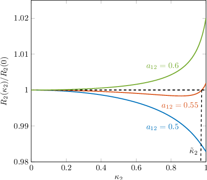
To illustrate the characterization provided in Lemma 3, we plot in Fig. 3 the rate of user 2 normalized by the proper signaling rate with examples for each of the three cases described in Lemma 3. We use and , which gives and . Notice that the three curves vary only slightly with because the three chosen values of (0.5, 0.55 and 0.6) are all close to the thresholds. Lemma 3 describes how the interference constraint shapes the dependency of the rate of user 2 on the degree of impropriety of its transmitted signal. Thus, if we drop the power budget constraint or, alternatively, if the power budget is sufficiently high, improper signaling outperforms proper signaling for all values of if , but only for some values of if , and it is always suboptimal if . It can be clearly seen now what the impact of the power budget constraint is. For the cases and , maximizes . However, increasing is only meaningful if it also permits increasing the transmit power. When the power budget constraint is considered, there may exist such that , hence increasing beyond that point does not permit a further increase in the transmit power (see Fig. 2). Therefore, when improper signaling will be optimal if , where is such that (see Fig. 3). On the other hand, improper signaling will be optimal for only if . This condition means that proper signaling does not permit transmitting at maximum power, thus there is still power left over, which can be exploited by improper signaling to improve the achievable rate.
With all these ingredients, we can derive a complete characterization of the optimality of improper signaling for this scenario and, consequently, of the Pareto-optimal region. Our main result is presented in the following theorem.
Theorem 1.
Let us define as in (26) and
| (27) |
where
| (28) |
and
| (29) | ||||
| (30) | ||||
| (31) |
Then, improper signaling is required to maximize if and only if
| (32) |
Furthermore, if this expression holds, the optimal circularity coefficient is
| (33) |
where is the minimum value of such that .
Proof.
Please refer to Appendix D. ∎
Before concluding this section, we introduce the following definition, which will be useful to describe the properties of the Pareto boundary.
Definition 2.
We call power-limited region all the points of the rate region boundary for which or, alternatively, . We call the remaining points of the rate region the interference-limited region, i.e., those for which or, alternatively, .
IV Discussion and numerical examples
This section provides a discussion on the derived characterization along with some numerical examples illustrating the most remarkable features of improper signaling in the Z-IC. Afterwards, the connection to related works in the literature is presented.
IV-A Optimal strategies
IV-A1 Optimality of proper signaling
As pointed out at the beginning of Section III, if proper signaling is the optimal strategy for one of the users, then it is also optimal for the other one. This means that any point of the region boundary is achieved by both users employing the same signaling scheme, i.e., either proper or improper, but not a combination of both.
IV-A2 Maximally improper signaling for both users is optimal at most at one boundary point
It can be noticed that there is at most one boundary point where both users simultaneously transmit a maximally improper signal, i.e., happens for no more than one Pareto-optimal point. This is due to the fact that, if the rate constraint (22) can be fulfilled for (which corresponds to the case ), then user 1 tolerates an infinite amount of maximally improper interference along the orthogonal direction (see second equation in (23)). However, user 2 may only increase its rate by increasing if it is operating below its power budget, since the only purpose of increasing is to increase as well. Because of this and because is a continuous function for , setting is always suboptimal when . However, this reasoning is not applicable when , since turns into a discontinuous function for . This is because, in that case, and . The intuition behind this behavior is that, when , the first user achieves its corresponding rate with a maximally improper signal, i.e., , only if the interference is orthogonal to the signal subspace, i.e., only when the second user also transmits a maximally improper signal. Consequently, must hold if and . Furthermore, since when , the condition is equivalent, by (16), to . That is, both users transmit maximally improper signals at the boundary point for which only if .
To illustrate this property, we provide two simulation examples. As a first example we consider the channel coefficient and the power budgets . Figure 4 shows the optimal circularity coefficients and the transmit power of user 2. In this example holds and because of that both users transmit maximally improper signals for . We can observe a discontinuity in the maximum transmit power of user 2, which will be explained later. Notice that, as approaches its maximum value of b/s/Hz, goes towards 0 while remains static at 1. Although this might seem to violate our statement in Section IV-A1, is only equal to zero when is, which only happens at b/s/Hz. In this case, the circularity coefficient is no longer meaningful since the transmit power is zero. Therefore, all the boundary points satisfy our claim, which is also clear according to the optimal value of in (16).

As a second example we consider . In this case , hence it is expected that there are no boundary points that are achieved by both users transmitting maximally improper signals. This can be observed in Fig. 5, which depicts the dependency of the circularity coefficients and transmit power on the rate, . At the boundary point for , user 2 chooses the transmit signal as maximally improper, but the optimal circularity coefficient of user 1 equals 0.8. In Fig. 5 we can also observe a discontinuity in the maximum transmit power and in the circularity coefficients at approximately b/s/Hz. This discontinuity is different from the one observed in Fig. 4 and can be explained as follows. At the point of the discontinuity we have . Furthermore, at this point . This means that maximally improper signaling achieves the same rate as proper signaling. Proper signaling starts outperforming improper signaling once increases beyond that point, in which case the optimal circularity coefficient jumps from to , and the maximum transmit power jumps then from to .

IV-A3 Relationship between and
Expression (16) also permits drawing insightful conclusions about the relationship between the circularity coefficients of both users. According to Theorem 1, implies . Hence, holds if and , i.e., when the signal-to-interference ratio (SIR) is greater than one. In such a case, it can be noticed that the signal transmitted by the first user is never chosen as maximally improper at any point of the Pareto boundary. This behavior can be clearly observed in Fig. 5. On the other hand, when , or, alternatively, when the SIR is equal to or lower than one, holds whenever , as can be seen in Fig. 4.
If the signal transmitted by user 1 is chosen as maximally improper for some points of the boundary, it will remain so as , or, in other words, as . This is because implies , so that, by (16), the first user will not decrease its circularity coefficient. However, once equals 1, which corresponds to the point , the degree of impropriety of the first user will then start decreasing with , since these rates are not achievable for .
IV-B Properties of the Pareto boundary
IV-B1 Behavior in the power-limited and interference-limited regions
The power-limited region, which refers to the power limitation of the second user, comprises all boundary points satisfying , or, alternatively, . In this region improper signaling is always optimal as long as the power budget is sufficiently high. In other words, the optimality of improper signaling is only determined by , which depends on and goes towards 0 as increases. Furthermore, user 1 can achieve its required rate with a maximally improper signal, i.e., with . In this case, the interference along the unused dimension does not have any impact on its achievable rate, therefore as . In the interference-limited region, user 1 must choose a circularity coefficient smaller than one to achieve the desired rate, and hence the tolerated interference is finite for all values of . As a result, the transmit power of the second user is eventually limited by as grows, which bounds the achievable rate. In other words, the optimality of improper signaling is eventually determined by , which is independent of the power budget .
IV-B2 Transition between power-limited and interference-limited regions
An interesting feature is that there may be abrupt changes in the achievable rate of user 2 when we shift from one region to the other, which are due to a jump in the tolerable interference power (as observed in Fig. 4). This can be explained as follows. In the power-limited region the transmit power always equals the power budget when improper signaling is optimal, i.e., if . However, in the interference-limited region the transmit power is dominated by the function when the power budget exceeds the value of that function, i.e., when . Hence, by using (16), it can be easily seen that , so that there may be a jump in the maximum transmit power, i.e., a discontinuity in the maximum transmit power of user 2 as a function of , from to whenever . That is, the lower the SIR, the more prominent the power jump is, whereas no jump will be observed when the SIR is equal to or greater than 1. This discontinuity in the maximum transmit power implies a similar jump in the maximum achievable rate of user 2, making . This is illustrated in Figs. 6 and 7, where the Pareto boundary of the rate region is depicted for the previously considered examples, i.e., and , respectively. We also depict in the figures the rate region boundary for proper signaling, and the enlargement of the rate region due to time sharing.

Figure 6 corresponds to a scenario where the SIR is below one, therefore we can observe that the Pareto boundary is discontinuous. As explained earlier, this is the result of a jump in the maximum transmit power of user 2, , which can also be observed in Fig. 4. Specifically, the maximum transmit power in the interference limited region equals , so there is a power jump from to . Notice that at the discontinuity, which approximately corresponds to b/s/Hz, all the rates in the half-open interval b/s/Hz are achievable but do not belong to the Pareto boundary as defined at the beginning of Section III. Similarly, all the rate pairs b/s/Hz and b/s/Hz are achievable but do not belong to the Pareto boundary. Therefore, these two line segments are plotted in dashed lines in Fig. 6.
The scenario corresponding to Fig. 7 presents an SIR greater than one. Because of that, the transition from the power-limited to the interference-limited regions presents no discontinuity as there is no jump in the transmit power at (see Fig. 5). Notice that the discontinuity in the maximum transmit power at b/s/Hz, which is due to falling below the threshold, does not cause a discontinuity in the Pareto boundary. As previously explained, this is because at that point holds, so proper and improper signaling achieve the same rate. Therefore, changes smoothly even though the transmit power and circularity coefficients jump.

Figures 6 and 7 also illustrate that the dependency of on in the power-limited region is different from the interference-limited region. Specifically, decreases more slowly with in the former. This is due to the fact that in these examples holds in the entire power-limited region, and therefore the decrease in is due to an increase in . In the interference-limited region, however, decreases towards 0 as increases, which has a stronger effect on the achievable rate. The transition between these two different behaviors leads to a sharp bend in the Pareto boundary, as observed in Figs. 6 and 7. It corresponds to the transition between the power-limited and interference-limited regions only if holds in the entire interference-limited region, and improper signaling is optimal in the power-limited region. This is because these conditions imply that is optimal at the transition point . Therefore, to satisfy the rate of the first user must decrease once we move into the interference-limited region, which changes the behavior of . If for some points in the interference-limited region, then is optimal at . Increasing while keeping constant permits achieving the required when we move into the interference-limited region until is reached. Hence the dependency of on will change at the value of such that , which is slightly shifted to the right. Figures 6 and 7 also show the enlargement of the rate region due to improper signaling. In these examples, the interference level is significant, so the achievable rate region by improper signaling is substantially larger than that of proper signaling, especially in the scenario shown in Fig. 6.
It is also worth highlighting that time sharing provides a substantial enlargement of the rate region for both proper and improper signaling, but there is still a significant gap between the performance of both strategies. In Fig. 6, the rate region achieved by improper signaling is convexified by time sharing between the extreme points of the Pareto boundary, which correspond to proper signaling transmissions, and the point at the transition between the power-limited and the interference-limited regions, where both users transmit maximally improper signals. By contrast, all the Pareto boundary points in the power-limited region belong to the convex hull in Fig. 7, and time sharing improves the performance only in the interference-limited region.
IV-B3 Operation regimes
Considering the possibly suboptimal approach of always treating interference as noise, we may distinguish the following operation regimes that account for the optimality of improper signaling.
- •
Strictly improper regime: If , we say the Z-IC is in the strictly improper regime. In this regime and treating interference as noise, all the Pareto-optimal points satisfying are achieved by improper signaling, i.e., .
- •
Selective improper/proper regime: If , we say the Z-IC is in the selective improper/proper regime. In this regime and treating interference as noise, only a subset of the Pareto-optimal points satisfying is achieved by improper signaling, i.e., .
- •
Strictly proper regime: If , we say the Z-IC is in the strictly proper regime. In this regime and treating interference as noise, all the Pareto-optimal points are achieved by proper signaling, i.e., .
Note that always belongs to the Pareto boundary and can only be achieved by proper signaling. Because of that, the operation regimes described above explain the optimal strategies for the boundary points satisfying . The strictly improper regime is obtained making use of Lemma 3, which establishes that is a sufficient condition for improper signaling to be optimal if proper signaling does not allow maximum power transmission, i.e., if . Therefore, holds for all boundary points satisfying . Furthermore, it can be easily checked that
| (34) |
Since is an increasing function, the condition for the optimality of improper signaling is fulfilled in the strictly improper regime for all Pareto-optimal points except for . An example of the operation in the strictly improper regime is given in Fig. 6 (and the corresponding Fig. 4). Figures 5 and 7 correspond to the selective improper/proper regime, and we can observe that improper signaling is optimal only in the interval b/s/Hz.
When we move from the power-limited region to the interference-limited region we have
| (35) |
where is such that . Therefore, proper signaling is the optimal strategy in the whole interference-limited region if . In such a case, benefits of improper signaling, if any, are limited to the power-limited region. Notice that, as increases, this condition converges to .
IV-C Relationship to previous work
Finally, we would like to connect our results to related works in the literature. In our previous work [14], we studied a similar scenario in the context of underlay cognitive radio. We considered the Z-IC with the restriction that the first user transmits only proper signals, i.e., . A characterization of the maximum achievable rate of user 2 was derived in terms of a threshold in . Specifically, improper signaling was shown to be optimal if . This threshold is strictly higher than the one obtained for the general Z-IC (it can easily be seen that ). This is in agreement with the fact that, if we let the first user optimize its circularity coefficient, the rate achieved by the second user can only increase.
The Z-IC was also considered in [17], and the transmit strategy that maximizes the sum-rate was derived in closed form based on the real-composite model. Although such a model is usually more convenient from an optimization point-of-view, it is not as insightful as the augmented complex model since some of the features of the improper signal are not easily captured. This is the case for the degree of impropriety, which is elegantly given by the circularity coefficient. We would like to stress that in [17] only one point of the rate region was characterized, whereas in this work we completely characterized the boundary of the rate region. Furthermore, since we consider the augmented complex model, we provided closed-form formulas for the circularity coefficients, thus providing a more insightful description of how improper signaling behaves in this scenario. Nevertheless, some of the conclusions drawn in [17] fall within our characterization of the rate region boundary. By looking at the structure of the sum-rate maximizing transmit strategies in [17, Eq. (31)], we observe that improper signaling is chosen when . This condition belongs to the strictly improper regime, and the solution presented in [17, Eq. (31)] can be seen as a special case of (33). Furthermore, according to [17], when improper signaling is preferred for the sum-rate maximization, the signal transmitted by one of the users is chosen as maximally improper, and the selection of the user depends on whether or not the condition holds. This is in agreement with our previous discussion, where we pointed out that the circularity coefficient of the first user is always equal to or smaller than that of the second user whenever the aforementioned condition is fulfilled. In such a case, the Pareto optimal point that corresponds to the sum-rate maximization is then the point that satisfies . Otherwise, if , the sum-rate is maximized when the first user transmits a maximally improper signal, and in this case the circularity coefficient of the second user is smaller than 1 except for .
The MIMO Z-IC with improper signaling has been considered in [18, 19]. Due to the inclusion of the spatial dimension, an analytical characterization of improper signaling similar to that of Theorem 1 becomes intractable. Notice that in the SISO Z-IC, the impropriety is completely described by the circularity coefficient. However, in the MIMO case, the description of the impropriety is by means of the complementary covariance matrix, which is characterized by a set of circularity coefficients and a unitary matrix [20]. Because of that, the authors proposed a heuristic scheme to design the complementary covariance matrix of the transmitted signal of user 2 such that it permits easy control of the degree of impropriety. An interesting aspect of [18, 19] is the fact that it does not completely stick to a particular model for the representation of improper signals. Thus, they use the real-composite model to optimize the transmission scheme of user 1, while they design the scheme of the second user by means of the augmented-complex formulation. Interestingly, the achievable rate regions obtained in [18, 19] have a shape similar to those in Figs. 6 and 7. This suggests that some of our conclusions for the single-antenna Z-IC might be extended to the more general MIMO Z-IC.
V Conclusion
We have analyzed the benefits of improper signaling in the single-antenna Z-IC. Under the assumption that interference is treated as Gaussian noise, we have derived a complete and insightful characterization of the Pareto boundary of the rate region, and the corresponding transmit powers and circularity coefficients in closed-form. This characterization has been derived by analyzing how the circularity coefficients affect the performance at the different boundary points. Specifically, we have shown that improper signaling is optimal when the interference coefficient exceeds a given threshold that depends on the rate achieved by the interfered user. We have shown that the rate region can be substantially enlarged by using improper signaling, especially when the relative level of interference is high.
Acknowledgements
The work of C. Lameiro and P. J. Schreier was supported by the German Research Foundation (DFG) under grant SCHR 1384/6-1. The work of I. Santamaria was supported by the Ministerio de Economia y Competitividad (MINECO), Spain, under projects RACHEL (TEC2013-47141-C4-3-R) and CARMEN (TEC2016-75067-C4-4-R).
The authors would like to thank the anonymous reviewers for their valuable comments, which have helped improve the quality of the paper.
Appendix A proof of Lemma 1
Let us first consider . In this case is equivalent, because of (18), to the quadratic inequality
| (36) |
which is convex and only has one positive root given by
| (37) |
Notice that the rate constraint of user 1 can only be fulfilled with a maximally improper signal if , that is, if user 1 can achieve its rate by transmitting all power over the real or imaginary part. This means that holds whenever , which implies . Hence, (37) can be simplified to , where is given by the second branch of (23). If , is equivalent to the quadratic inequality
| (38) |
The equivalent power constraint will then be given by one of the roots of this equation. In order to determine which one of the two roots must be considered we can use the fact that is decreasing in . This means that at least one of the roots will violate the condition , with given by (16). The roots of (38) are
|
|
(39) |
Notice that . Therefore, if (38) is convex, i.e., if , (38) has one negative and one positive root, and the equivalent power constraint will be given by the latter if it satisfies . Otherwise, the rate expression for must be considered. If (38) is concave, both roots can be either positive, negative, or complex. For the last two cases, none of them satisfies , so the equivalent power constraint must be obtained through the expression for . If the two roots are positive, the monotonicity of in is not fulfilled for the largest root, hence the equivalent power constraint is determined by the smallest root. For all these cases, the root that must be considered is obtained by taking the positive square root in (39) which, after some manipulations, yields , with being given by the first branch of (23). This concludes the proof.
Appendix B Proof of Lemma 2
Through (24), the derivative of with respect to is non-negative if
| (40) |
Let us first consider . In this case we have
| (41) |
Plugging (41) into (40) we obtain
| (42) |
which holds for all values of . If , (38) holds with equality for . Therefore, evaluating (38) at and taking the derivative with respect to yields
|
|
(43) |
Plugging (43) into (40) we obtain
| (44) |
The denominator in this expression can be shown to be positive as follows. Since we are assuming that holds, we have, through (23), that , hence it is positive. Consequently, we obtain
| (45) |
where , which does not depend on as can be seen from (23). Let be such that the right-hand side of (45) holds with equality. Since for , increases with and, consequently, the right-hand side of (45) holds with strict inequality when . As a result, the derivative of is positive whenever , which concludes the proof.
Appendix C Proof of Lemma 3
By Lemma 2, increases monotonically in as long as for . Clearly, is also zero at this point, thus we can apply (45), yielding
| (46) |
which proves the first case. In the second case, improper signaling outperforms proper signaling only for . By Lemma 2 we also know that, if improper signaling outperforms proper signaling for , then the rate improvement will be strictly positive for . Therefore, when holds, there must be such that and for all . To evaluate when holds, we first consider the boundary points satisfying . Since at these points user 1 can achieve its required rate with a maximally improper signal, i.e., with , we have that . Consequently, is always fulfilled for , which yields the second branch of (26). For the boundary points satisfying , holds. Therefore, using the corresponding branch in (23) for yields
| (47) |
Using this expression and (24), holds if
| (48) |
which yields
| (49) |
Taking into account that , we have
|
|
(50) |
which yields the first branch of (26). Finally, if then we have and, by Lemma 2, for all . This yields the third case and concludes the proof.
Appendix D Proof of Theorem 1
By Lemma 3, improper signaling can only be optimal if . However, this condition is not sufficient, since it does not take the power budget constraint into account. Firstly, since increasing can improve the rate only if this permits increasing the transmit power as well, we must have that . This is equivalent to
| (51) |
If is greater than this quantity and also than , we know by Lemma 3 that is optimal if . Otherwise, it is clear that, if improper signaling is optimal, then the optimal circularity coefficient will satisfy . Let us denote this circularity coefficient as . Then, using (24) we have
| (52) |
Therefore, we have to evaluate the condition for , with , fulfilling the above expression. Let us first consider the case . From (23), we have that
| (53) |
Plugging this expression into (52) we have the condition
| (54) |
which, after some manipulations, yields the quadratic inequality
| (55) |
where and are respectively given by (30) and (31). This quadratic expression is convex and has at most one positive root. Hence, the condition on is given by the largest root, which is
| (56) |
This expression, however, is only applicable if holds for the above threshold. Using (16), holds if
| (57) |
Otherwise we have , thus we have to obtain using the first branch in (23) (or, alternatively, taking equality in (38) with ), which yields
|
|
(58) |
Plugging this expression into (52) we obtain
| (59) |
which, after some manipulations, yields
| (60) |
Since the above quadratic expression is convex, we have to consider the largest root. As expected, one of the roots is
| (61) |
which corresponds to the maximum power allowed by proper signaling. Since we have already considered this threshold in (51), we have to use the second root, which can be simplified to
| (62) |
If the above root is the largest one, the inequality (60) is satisfied when exceeds this value, which yields the condition
| (63) |
Combining (51)-(63) we obtain that must hold for improper signaling to be optimal, with given by (27). However, this condition is only valid if . Consequently, improper signaling will be optimal if and only if is greater than the dominating threshold, i.e., if and only if . If this expression is satisfied, then by Lemma 3 must be increased until , thus the optimal circularity coefficient is given by (33). This concludes the proof.
References
- [1] F. D. Neeser and J. L. Massey, “Proper complex random processes with applications to information theory,” IEEE Transactions on Information Theory, vol. 39, no. 4, pp. 1293–1302, Jul. 1993.
- [2] V. Cadambe, S. Jafar, and C. Wang, “Interference alignment with asymmetric complex signaling—settling the Høst-Madsen-Nosratinia conjecture,” IEEE Transactions on Information Theory, vol. 56, no. 9, pp. 4552–4565, Sep. 2010.
- [3] C. Lameiro and I. Santamaría, “Degrees-of-freedom for the 4-user SISO interference channel with improper signaling,” in Proc. IEEE Int. Conf. Comm., Budapest, Hungary, Jun. 2013.
- [4] C. Wang, T. Gou, and S. A. Jafar, “On optimality of linear interference alignment for the three-user MIMO interference channel with constant channel coefficients,” [Online]. Available: http://escholarship.org/uc/item/6t14c361, 2011.
- [5] H.-Y. Shin, S.-H. Park, H. Park, and I. Lee, “A new approach of interference alignment through asymmetric complex signaling and multiuser diversity,” IEEE Transactions on Wireless Communications, vol. 11, no. 3, pp. 880–884, Mar. 2012.
- [6] L. Yang and W. Zhang, “Interference alignment with asymmetric complex signaling on MIMO X channels,” IEEE Transactions on Communications, vol. 62, no. 10, pp. 3560–3570, Oct. 2014.
- [7] Z. Ho and E. Jorswieck, “Improper Gaussian signaling on the two-user SISO interference channel,” IEEE Transactions on Wireless Communications, vol. 11, no. 9, pp. 3194–3203, Sep. 2012.
- [8] Y. Zeng, C. Yetis, E. Gunawan, Y. Guan, and R. Zhang, “Transmit optimization with improper Gaussian signaling for interference channels,” IEEE Transactions on Signal Processing, vol. 61, no. 11, pp. 2899–2913, Jun. 2013.
- [9] Y. Zeng, R. Zhang, E. Gunawan, and Y. Guan, “Optimized transmission with improper Gaussian signaling in the -user MISO interference channel,” IEEE Transactions on Wireless Communications, vol. 12, no. 12, pp. 6303–6313, Dec. 2013.
- [10] H. Nguyen, R. Zhang, and S. Sun, “Improper signaling for symbol error rate minimization in -user interference channel,” IEEE Transactions on Communications, vol. 63, no. 3, pp. 857–869, Mar. 2015.
- [11] S. Lagen, A. Agustin, and J. Vidal, “Coexisting linear and widely linear transceivers in the MIMO interference channel,” IEEE Transactions on Signal Processing, vol. 64, no. 3, pp. 652–664, Feb. 2016.
- [12] C. Hellings, M. Joham, and W. Utschick, “QoS feasibility in MIMO broadcast channels with widely linear transceivers,” IEEE Signal Processing Letters, vol. 20, no. 11, pp. 1134–1137, Nov. 2013.
- [13] C. Kim, E.-R. Jeong, Y. Sung, and Y. H. Lee, “Asymmetric complex signaling for full-duplex decode-and-forward relay channels,” in Proceedings of the International Conference on ICT Convergence (ICTC), Oct. 2012, pp. 28–29.
- [14] C. Lameiro, I. Santamaría, and P. J. Schreier, “Benefits of improper signaling for underlay cognitive radio,” IEEE Wireless Communications Letters, vol. 4, pp. 22—25, Feb. 2015.
- [15] C. Lameiro, I. Santamaría, and P. Schreier, “Analysis of maximally improper signalling schemes for underlay cognitive radio,” in Proceedings of the IEEE International Conference on Communications, London, UK, Jun. 2015.
- [16] O. Amin, W. Abediseid, and M.-S. Alouini, “Outage performance of cognitive radio systems with improper Gaussian signaling,” in Proceedings of the IEEE International Symposium on Information Theory (ISIT), Hong Kong, China, Jun. 2015, pp. 1851–1855.
- [17] E. Kurniawan and S. Sun, “Improper Gaussian signaling scheme for the Z-interference channel,” IEEE Transactions on Wireless Communications, vol. 14, no. 7, pp. 3912–3923, Jul. 2015.
- [18] S. Lagen, A. Agustin, and J. Vidal, “Improper Gaussian signaling for the Z-interference channel,” in Proceedings of the IEEE International Conference on Acoustics, Speech and Signal Processing (ICASSP), Florence, Italy, May 2014, pp. 1145–1149.
- [19] ——, “On the superiority of improper Gaussian signaling in wireless interference MIMO scenarios,” IEEE Transactions on Communications, vol. 64, no. 8, pp. 3350–3368, Aug. 2016.
- [20] P. J. Schreier and L. L. Scharf, Statistical signal processing of complex-valued data: the theory of improper and noncircular signals. Cambridge, U.K.: Cambridge Univ. Press, 2010.
- [21] T. Adali, P. J. Schreier, and L. L. Scharf, “Complex-valued signal processing: The proper way to deal with impropriety,” IEEE Transactions on Signal Processing, vol. 59, no. 11, pp. 5101–5125, Nov. 2011.
- [22] G. Tauböck, “Complex-valued random vectors and channels: Entropy, divergence, and capacity,” IEEE Transactions on Information Theory, vol. 58, no. 5, pp. 2729–2744, May 2012.
- [23] W. Gerstacker, R. Schober, and A. Lampe, “Receivers with widely linear processing for frequency-selective channels,” IEEE Transactions on Communications, vol. 51, no. 9, pp. 1512–1523, Sep. 2003.
- [24] S. Buzzi, M. Lops, and S. Sardellitti, “Widely linear reception strategies for layered space-time wireless communications,” IEEE Transactions on Signal Processing, vol. 54, no. 6, pp. 2252–2262, Jun. 2006.
- [25] P. Chevalier and F. Pipon, “New insights into optimal widely linear array receivers for the demodulation of BPSK, MSK, and GMSK signals corrupted by noncircular interferences—application to SAIC,” IEEE Transactions on Signal Processing, vol. 54, no. 3, pp. 870–883, Mar. 2006.
- [26] R. Schober, W. Gerstacker, and L.-J. Lampe, “Data-aided and blind stochastic gradient algorithms for widely linear MMSE MAI suppression for DS-CDMA,” IEEE Transactions on Signal Processing, vol. 52, no. 3, pp. 746–756, Mar. 2004.
- [27] B. W. Han and J. H. Cho, “Capacity of second-order cyclostationary complex Gaussian noise channels,” IEEE Transactions on Communications, vol. 60, no. 1, pp. 89–100, Jan. 2012.
- [28] J. Yeo and J. H. Cho, “Asymptotic frequency-shift properizer for block processing of improper-complex second-order cyclostationary random processes,” IEEE Transactions on Information Theory, vol. 60, no. 7, pp. 4083–4100, Jul. 2014.
- [29] J. Yeo, J. H. Cho, and J. S. Lehnert, “Joint transmitter and receiver optimization for improper-complex second-order stationary data sequence,” Journal of Communications and Networks, vol. 17, no. 1, pp. 1–11, Feb. 2015.
- [30] J. Yeo, B. W. Han, J. H. Cho, and J. S. Lehnert, “Capacity of an orthogonal overlay channel,” IEEE Transactions on Wireless Communications, vol. 14, no. 11, pp. 6111–6124, Nov. 2015.
- [31] M. Kim, J. H. Cho, and J. S. Lehnert, “Asymptotically optimal low-complexity SC-FDE with noise prediction in data-like improper-complex interference,” IEEE Transactions on Wireless Communications, vol. 15, no. 3, pp. 2090–2103, Mar. 2016.
- [32] M. Costa, “On the Gaussian interference channel,” IEEE Transactions on Information Theory, vol. 31, no. 5, pp. 607–615, Sep. 1985.
- [33] R. Prasad, S. Bhashyam, and A. Chockalingam, “On the sum-rate of the Gaussian MIMO Z channel and the Gaussian MIMO X channel,” IEEE Transactions on Communications, vol. 63, no. 2, pp. 487–497, Feb. 2015.
- [34] H. Sato, “The capacity of the Gaussian interference channel under strong interference,” IEEE Transactions on Information Theory, vol. 27, no. 6, pp. 786–788, Nov. 1981.
- [35] H. Song, J. Y. Ryu, and W. Choi, “Characterization of the Pareto boundary for the two-user symmetric Gaussian interference channel,” IEEE Transactions on Communications, vol. 62, no. 8, pp. 2812–2824, Aug. 2014.
- [36] C. Hellings and W. Utschick, “Block-skew-circulant matrices in complex-valued signal processing,” IEEE Transactions on Signal Processing, vol. 63, no. 8, pp. 2093–2107, Apr. 2015.
- [37] E. A. Jorswieck, E. G. Larsson, and D. Danev, “Complete characterization of the pareto boundary for the MISO interference channel,” IEEE Transactions on Signal Processing, vol. 56, no. 10, pp. 5292–5296, Oct. 2008.