Finding Planted Subgraphs with Few Eigenvalues using the Schur-Horn Relaxation Thanks: The authors were supported in part by NSF Career award CCF-1350590 and by Air Force Office of Scientific Research grant FA9550-14-1-0098.
Abstract
Extracting structured subgraphs inside large graphs – often known as the planted subgraph problem – is a fundamental question that arises in a range of application domains. This problem is NP-hard in general, and as a result, significant efforts have been directed towards the development of tractable procedures that succeed on specific families of problem instances. We propose a new computationally efficient convex relaxation for solving the planted subgraph problem; our approach is based on tractable semidefinite descriptions of majorization inequalities on the spectrum of a symmetric matrix. This procedure is effective at finding planted subgraphs that consist of few distinct eigenvalues, and it generalizes previous convex relaxation techniques for finding planted cliques. Our analysis relies prominently on the notion of spectrally comonotone matrices, which are pairs of symmetric matrices that can be transformed to diagonal matrices with sorted diagonal entries upon conjugation by the same orthogonal matrix.
Keywords— convex optimization; distance-regular graphs; induced subgraph isomorphism; majorization; orbitopes; semidefinite programming; strongly regular graphs.
1 Introduction
In application domains ranging from computational biology to social data analysis, graphs are frequently used to model relationships among large numbers of interacting entities. A commonly encountered question across many of these application domains is that of identifying structured subgraphs inside larger graphs. For example, identifying specific motifs or substructures inside gene regulatory networks is useful in revealing higher-order biological function [3, 16, 31]. Similarly, extracting completely connected subgraphs in social networks is useful for determining communities of people that are mutually linked to each other [30, 33, 35]. In this paper, we propose a new algorithm based on convex optimization for finding structured subgraphs inside large graphs, and we give conditions under which our approach succeeds in performing this task.
Formally, suppose and are graphs11 1 Throughout this paper we consider undirected, unweighted, loopless graphs. on nodes and nodes (here ), respectively, with the following property: there exists a subset of vertices with such that the induced subgraph of corresponding to the vertex set is isomorphic to . The planted subgraph problem is to identify the vertex subset given the graphs and ; see Figure 1 for an example. The decision version of the planted subgraph problem is known as the induced subgraph isomorphism problem in the theoretical computer science literature, and it has been shown to be NP-hard [27]. Nevertheless, as this problem arises in a wide range of application domains as described above, significant efforts have been directed towards the development of computationally tractable procedures that succeed on certain families of problem instances. Much of the focus of this attention has been on the special case of the planted clique problem in which the subgraph is fully connected. Alon et al. [1] and Feige and Krauthgamer [21] developed a spectral algorithm for the planted clique problem, and subsequently Ames and Vavasis [2] described an approach based on semidefinite programming with similar performance guarantees to the earlier work based on spectral algorithms. Conceptually, these methods are based on a basic observation about the spectrum of a clique, namely that the adjacency matrix of a clique on nodes has two distinct eigenvalues, one with multiplicity equal to one and the other with multiplicity equal to . We describe a new semidefinite programming technique that generalizes the method of Ames and Vavasis [2] to planted subgraphs that are not fully connected, with the spectral properties of playing a prominent role in our algorithm and our analysis.


1.1 Our Contributions
Let and represent the adjacency matrices of and of , with denoting the space of real symmetric matrices. Given any matrix , we let for denote an symmetric matrix with the leading principal minor of order equal to and all the other entries equal to zero. The following combinatorial optimization problem is a natural first approach to phrase the planted subgraph problem in a variational manner:
| (1) | ||||
Assuming that there is no other subgraph of that is isomorphic to , one can check that the optimal solution of this problem identifies the vertices whose induced subgraph in is isomorphic to , i.e., the unique optimal solution is equal to zero everywhere except for the principal minor corresponding to the indices in and for some permutation matrix . However, solving (1) is intractable in general. Replacing the combinatorial constraint with the convex constraint does not lead to a tractable problem as checking membership in the polytope is intractable for general planted graphs (unless P NP).
We describe next a convex outer approximation of the set that leads to a tractable convex program. For any matrix , the Schur-Horn orbitope is defined as [38]:
| (2) |
The term ‘orbitope’ was coined by Sanyal, Sottile, and Sturmfels in their work on convex hulls of orbits generated by the actions of groups, and the Schur-Horn orbitope was so named by these authors due to its connection to the Schur-Horn theorem in linear algebra [38]. In combinatorial optimization, approximations based on replacing permutations matrices by orthogonal matrices have also been employed to obtain bounds on the Quadratic Assignment Problem [22]. The set depends only on the eigenvalues of , and it is clearly an outer approximation of the set . Crucially for our purposes, the Schur-Horn orbitope for any has a tractable semidefinite description via majorization inequalities on the spectrum of a symmetric matrix [6, 38]; see Section 4.1. Hence, we propose the following tractable semidefinite programming relaxation for the planted subgraph problem:
| () | ||||
Here is the identity matrix. We refer to this convex program as the Schur-Horn relaxation, and this problem can be solved to a desired precision in polynomial time. This relaxation only requires knowledge of the eigenvalues of the planted graph . The parameter is to be specified by the user, and we discuss suitable choices for in the sequel. Note that changing to in the constraints of (1) essentially leaves that problem unchanged (the nonzero principal minor of the optimal solution simply changes from to ). However, the additional degree of freedom provided by the parameter plays a more significant role in the Schur-Horn relaxation as it allows for shifts of the spectrum of to more favorable values, which is essential for the solution of various planted subgraph problems; see Section 2.1 for further details, as well as the experiments in Section 4 for numerical illustrations. We say that the Schur-Horn relaxation succeeds in recovering the planted subgraph if the optimal solution satisfies the following conditions: the optimal solution is unique, the submatrix for some permutation matrix , and the remaining entries of are equal to zero.
In Section 2 we study the geometric properties of the Schur-Horn orbitope as these pertain to the optimality conditions of the Schur-Horn relaxation. Our analysis relies prominently on the notion of spectrally comonotone matrices, which refers to a pair of symmetric matrices that can be transformed to diagonal matrices with sorted diagonal entries upon conjugation by the same orthogonal matrix. Spectral comonotonicity is a more restrictive condition than simultaneous diagonalizability, and it enables a precise characterization of the normal cones at extreme points of the Schur-Horn orbitope (Proposition 6). This discussion leads directly to the central observation of our paper that the Schur-Horn relaxation is useful for finding planted graphs that consist of few distinct eigenvalues. Cliques form the simplest examples of such graphs as their spectrum consists of two distinct eigenvalues. There are numerous other graph families whose spectrum consists of few distinct eigenvalues, and the study of such graphs is a significant topic in graph theory [8, 18, 19, 34, 41, 42, 43]. For example, strongly regular graphs are (an infinite family of) regular graphs with three distinct eigenvalues; the Clebsch graph of Figure 1 is a strongly regular graph on nodes with eigenvalues in the set and degree equal to five. For a more extensive list of graphs with few eigenvalues, see Section 2.2.
We state and prove the main theoretical result of this paper in Section 3.4 – see Theorem 1. If the planted subgraph and its complement are both symmetric – and its complement are both vertex- and edge-transitive – and if is connected, then this theorem takes on a simpler form (Corollary 20). Specifically, the success of the Schur-Horn relaxation ( P ) relies on the existence of a suitable eigenspace of . Concretely, let denote the projection onto , and let denote the coherence of . Assuming that the edges in outside the induced subgraph are placed independently and uniformly at random with probability (i.e., the Erdős-Rényi random graph model), we show in Corollary 20 that the Schur-Horn relaxation ( P ) with parameter22 2 In our experiments in Section 4, we set equal to the eigenvalue of with the largest multiplicity. See Section 3 for further discussion. (the eigenvalue associated to ) succeeds with high probability provided:
The coherence parameter lies in , and it appears prominently in results on sparse signal recovery via convex optimization [17]. In analogy to that literature, a small value of is useful in our context (informally) to ensure that the planted graph looks sufficiently ‘different’ from the remainder of (see Section 3 for details). Thus, the Schur-Horn relaxation succeeds if the planted graph consists of few distinct eigenvalues that are well-separated, and in which one of the eigenspaces has a small coherence parameter associated to it. For more general non-symmetric graphs, our main result (Theorem 1) is stated in terms of a parameter associated to an eigenspace of called the combinatorial width, which roughly measures the average conditioning over all minors of of a certain size.
Specialization to the planted clique problem
The sum of the adjacency matrix of a clique and the identity matrix has rank equal to one, and consequently the planted clique problem may be phrased as one of identifying a rank-one submatrix inside a larger matrix (up to shifts of the diagonal by the identity matrix). In her thesis [20], Fazel proposed the nuclear norm as a tractable convex surrogate for identifying low-rank matrices in convex sets, and subsequent efforts provided theoretical support for the effectiveness of this relaxation in a range of rank minimization problems [12, 36]. Building on these ideas, Ames and Vavasis [2] proposed a nuclear norm minimization approach for the planted clique problem. The Schur-Horn relaxation ( P ) specializes to the relaxation in [2] when is the clique. Specifically, letting denote the adjacency matrix of a -clique, one can check that:
| (3) |
As the nuclear norm of a positive semidefinite matrix is equal to its trace, the Schur-Horn orbitope is simply a face of the nuclear norm ball in scaled by a factor . Thus, the Schur-Horn relaxation ( P ) with is effectively a nuclear norm relaxation when the planted subgraph of interest is the clique.33 3 The nuclear norm relaxation in [2] is formulated in a slightly different fashion compared to the Schur-Horn relaxation ( P ) for the case of the planted clique; specifically, one can show that our relaxation succeeds whenever the nuclear norm relaxation in [2] succeeds. Further, our main result (Theorem 1) can be specialized to the case of a planted clique to obtain the main result in [2]; see Corollary 21.
1.2 Paper Outline
In Section 2 we discuss the geometric properties of the Schur-Horn orbitope and their connection to the optimality conditions of the Schur-Horn relaxation, along with an extensive list of families of graphs with few eigenvalues. Section 3 contains our main theoretical results, while in Section 4 we demonstrate the utility of the Schur-Horn relaxation in practice via numerical experiments. We conclude in Section 5 with a discussion of further research directions.
Notation
The normal cone at a point for a closed, convex set is denoted by and it is the collection of linear functionals that attain their maximal value over at [37]. The projection operator onto a subspace is denoted by . The restriction of a linear map to an invariant subspace of is denoted by . The orthogonal complement of a subspace is denoted by . The notation denotes the dimension of a subspace . The eigengap of a symmetric matrix associated to an invariant subspace of is defined as:
The smallest and largest eigenvalues of a symmetric matrix are represented by and , respectively. The norms , and denote the vector norm, the matrix operator/spectral norm, and the matrix Frobenius norm, respectively. The vector denotes the all-ones vector of length . We denote the identity matrix of size by . The matrix denotes the matrix whose rows are the rows of indexed by , so that the rows of are the rows of indexed by for any . The matrix denotes the principal minor of indexed by the set . The group of orthogonal matrices is denoted by . The set specifies the relative interior of any set . The column space of a matrix is denoted by . The quantity denotes the usual expected value, where the distribution is clear from context.
2 Geometric Properties of the Schur-Horn Orbitope
In this section, we analyze the optimality conditions of the Schur-Horn relaxation from a geometric perspective. In particular, the notion of a pair of spectrally comonotone matrices plays a central role in our development, and we elaborate on this point in the next subsection. Based on this discussion, we observe that the Schur-Horn relaxation is especially useful for finding planted graphs consisting of few distinct eigenvalues, and we give examples of graphs with this property in Section 2.2. The main theoretical results formalizing the utility of the Schur-Horn relaxation are presented in Section 3.
2.1 Optimality Conditions of the Schur-Horn Relaxation
We state the optimality conditions of the Schur-Horn relaxation in terms of the normal cones at extreme points of the Schur-Horn orbitope:
Lemma 1.
Consider a planted subgraph problem instance in which the nodes of and are labeled so that the leading principal minor of of order is equal to . Suppose there exists a matrix with the following properties:
- 1.
,
- 2.
Then the Schur-Horn relaxation succeeds at identifying the planted subgraph inside the larger graph , i.e., the unique optimal solution of the convex program ( P ) is .
Proof.
The assumption on the node labeling is made purely for the sake of notational convenience in our analysis (to avoid clutter in having to keep track of additional permutations), and our algorithmic methodology does not rely on such a labeling. Based on this characterization of the optimality conditions, the success of the Schur-Horn relaxation relies on the existence of a suitable dual variable that satisfies two conditions. The first of these conditions relates to the structure of the noise edges in , while the second condition relates to the structure of the planted graph via the normal cone . From the viewpoint of Lemma 1, favorable problem instances for the Schur-Horn relaxation are, informally speaking, those in which there are not too many noise edges in (implying a less restrictive first requirement on ) and in which the normal cone is large (entailing a more flexible second condition for ). The interplay between these two conditions forms the basis of our analysis and results presented in Section 3. In the remainder of the present section, we investigate spectral properties of planted graphs that result in a large normal cone .
The normal cones at the extreme points of the Schur-Horn orbitope are conveniently described based on the following notion (see Proposition 6 in the sequel):
Definition 2.
A pair of symmetric matrices is spectrally comonotone if there exists an orthogonal matrix such that and are both diagonal matrices with the diagonal entries sorted in nonincreasing order.
The stipulation that two matrices be spectrally comonotone is a stronger condition than the requirement that the matrices be simultaneously diagonalizable, due to the additional restriction on the ordering of the diagonal entries upon conjugation by an orthogonal matrix.
Example 3.
Consider the matrices . The matrices and are spectrally comonotone, while and are only simultaneously diagonalizable and are not spectrally comonotone.
As Proposition 1 states the optimality conditions of the Schur-Horn relaxation in terms of the relative interiors of normal cones at extreme points of the Schur-Horn orbitope, we need the following “strict” analog of spectral comonotonicity:
Definition 4.
A matrix is strictly spectrally comonotone with a matrix , if for every that is simultaneously diagonalizable with , there exists such that and are spectrally comonotone.
Strict spectral comonotonicity is more restrictive than spectral comonotonicity. Further, the definition of strict spectral comonotonocity is not a symmetric one, unlike that of spectral comonotonicity, i.e., even if is strictly spectrally comonotone with , it may be that is not strictly spectrally comonotone with .
Example 5.
Consider the matrices . The matrix is strictly spectrally comonotone with the matrix , but is not strictly spectrally comonotone with .
The following result provides a characterization of normal cones at extreme points of the Schur-Horn orbitope in terms of spectrally comonotone matrices:
Proposition 6.
For any matrix and the associated Schur-Horn orbitope , the normal cone and its relative interior at an extreme point of are given by:
Note
For any matrix , the extreme points of are the elements of the set , as each of the matrices for has the same Frobenius norm.
Proof.
Let without loss of generality. We have that:
The last line follows from the inequality . Considering the case of equality in the Von Neumann trace inequality [45], we have that if and only if and are spectrally comonotone. The claim about the relative interior of the normal cone follows immediately from the definition of strict spectral comonotonicity. ∎
If a matrix has few distinct eigenvalues, the normal cone at an extreme point (for orthogonal) of is larger as there are many more matrices that are spectrally comonotone with . Based on Proposition 6, this observation suggests that planted graphs with few distinct eigenvalues have large normal cones , and such graphs are especially amenable to recovery in planted subgraph problems via the Schur-Horn relaxation. We make this insight more precise with our analysis in Section 3.4. Proposition 6 also points to the utility of employing the parameter in the Schur-Horn relaxation ( P ). Specifically, multiplicities in the spectrum of the matrix may be increased via suitable choices of , which in turn makes the normal cone larger. In particular, setting equal to an eigenvalue of increases the multiplicity of zero as an eigenvalue of . As detailed in Section 3, the success of the Schur-Horn relaxation relies on the existence of an eigenspace of with small coherence parameter, and the appropriate choice of is the eigenvalue associated to . In our experiments in Section 4, we set equal to the eigenvalue of with largest multiplicity, so that the multiplicity of zero as an eigenvalue of is as large as possible.
To conclude, we record an observation on spectral comonotonocity that is useful in Section 3. The claim is straightforward and therefore we omit the proof.
Lemma 7.
A pair of symmetric matrices is spectrally comonotone if and only if and are simultaneously diagonalizable and
| (4) |
where for are eigenspaces of ordered such that the corresponding eigenvalues of are decreasing. Further, is strictly spectrally comonotone with if and only if and are simultaneously diagonalizable and each of the inequalities (4) holds strictly.
2.2 Graphs with Few Eigenvalues
Building on the preceding section, we give examples of families of graphs consisting of few distinct eigenvalues. Such graphs have received much attention due to their connections to topics in combinatorics and design theory such as pseudorandomness [28] and association schemes [5, 23].
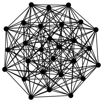


Triangular graphs
The triangular graph of order is the line graph of the complete graph on nodes. The graph has nodes and it has the three distinct eigenvalues (with multiplicity ), (with multiplicity ), and (with multiplicity ). Figure 2 gives two examples.
Kneser graphs
A Kneser graph is a graph on nodes, each corresponding to an -element subset of elements, and it consists of edges between those pairs of vertices for which the corresponding subsets are disjoint. The graph is the complete graph on nodes and the graph is the Petersen graph (Figure 2). The Kneser graph has distinct eigenvalues in general.


Paley graphs
Let be a prime power such that . The Paley graph on nodes is an undirected graph formed by connecting pairs of nodes if the difference is a square in the finite field . Note that is a square if and only if is a square as is a square in . Paley graphs have eigenvalues (with multiplicity ), (with multiplicity ), and (with multiplicity ). Paley graphs are also examples of pseudorandom graphs as they exhibit properties similar to random graphs (in the limit of large ) [28]. Figure 3 shows the three smallest Paley graphs.


Strongly regular graphs
These are regular graphs with the property that every pair of adjacent vertices has the same number of common neighbors and every pair of non-adjacent vertices has the same number of common neighbors, for some integers [7]. Strongly regular graphs that are connected have three distinct eigenvalues; conversely, connected and regular graphs with three distinct eigenvalues are necessarily strongly regular. The triangular graphs, Kneser graphs with parameter and the Paley graphs mentioned above are examples of strongly regular graphs. The Clebsch graph shown in Figure 1(a) in the introduction is also a strongly regular graph with degree and eigenvalues (with multiplicity ), (with multiplicity ), and (with multiplicity ). The generalized quadrangle graphs shown in Figure 4 are additional examples of strongly regular graphs. Strongly regular graphs form a significant topic in graph theory due to their many regularity properties [10, 11, 39].


Other examples
Unlike regular graphs with three distinct eigenvalues, graphs with four (or more) eigenvalues do not appear to have a simple combinatorial characterization [42]. Nonetheless, there are many constructions of such graphs in the literature [26, 41, 42], most notably those derived from distance-regular graphs [9] and from association schemes. Graphs from association schemes of class- have at most eigenvalues, and therefore several examples of graphs with four eigenvalues come from -class association schemes [14, 32]. The two graphs shown in Figure 5 are obtained from the Hamming scheme.
3 Recovering Subgraphs Planted in Erdős-Rényi Random Graphs
In this section we discuss our theoretical results on the performance of the Schur-Horn relaxation in recovering subgraphs planted inside Erdős-Rényi random graphs. Formally, suppose without loss of generality as in the previous section that the nodes of and of are labeled so that the leading principal minor of of order is equal to . The Erdős-Rényi model for the planted subgraph problem specifies a distribution on the edges in the remainder of the graph via a probability parameter ; for each with and , the graph contains an edge between nodes and with probability (independent of the other edges):
We begin with a sufficient condition for the optimality condition described in Lemma 1, which suggests a natural approach for constructing suitable dual variables for certifying optimality. These sufficient conditions point to the importance of the existence of an eigenspace of with certain properties to the success of the Schur-Horn relaxation; these properties are discussed in Section 3.2. In Section 3.4 we state and prove the main theorem (Theorem 1) of this paper, with Section 3.5 giving specializations of this result (e.g., to the planted clique problem).
3.1 A Simpler Sufficient Condition for Optimality
The following proposition provides a simpler set of conditions than those in Lemma 1 on dual variables that certify the success of the Schur-Horn relaxation. This result continues to be deterministic in nature, and the probabilistic aspects of our analysis – due to the Erdős-Rényi model – appear in the sequel.
Proposition 8.
Consider a planted subgraph problem instance in which the nodes of and are labeled so that the leading principal minor of of order is equal to . Suppose there exists an eigenspace of with eigenvalue , and suppose there exists a matrix with submatrices such that the the following conditions are satisfied:
-
, if or if ,
-
The submatrix is strictly spectrally comonotone with ,
-
and ,
-
Each column of the submatrix lies in the subspace ,
-
.
Then the Schur-Horn relaxation ( P ) with parameter succeeds at identifying the planted subgraph inside the larger graph .
Proof.
We establish this result by showing that the given matrix satisfies the requirements of Lemma 1. The first condition of Lemma 1 is identical to that of this proposition, and therefore it is satisfied. We prove next that the remaining conditions of this proposition ensure that the second requirement of Lemma 1 is also satisfied, i.e., . Based on Proposition 6, this entails showing that is strictly spectrally comonotone with . Our strategy is to employ Lemma 7.
Let be the eigenspaces of ordered such that the corresponding eigenvalues are strictly decreasing, and suppose for some . As is an eigenvalue of , one can check that the eigenspaces of are (with corresponding eigenvalues ) and (with eigenvalue ). We now need to show that and are simultaneously diagonalizable, and that for .
First, as is an eigenspace of with eigenvalue and as every column of belongs to , one can check that . Further, from Lemma 7 we note that and are simultaneously diagonalizable because is strictly spectrally comonotone with (and hence with ). From these two observations one can check that and commute with each other, and therefore are simultaneously diagonalizable.
As and are simultaneously diagonalizable, we have that the eigenspaces of are invariant subspaces of . Similarly, as is strictly spectrally comonotone with , the eigenspaces are invariant subspaces of . Based on the structure of these eigenspaces as described above, one can check that the eigenvalues of are equal to those of for each . Hence, for and for .
All that remains to be verified is that and that . As each column of belongs to and as , we have for that:
| (5) |
Consequently, recalling that we have:
The first inequality follows from (5), the second inequality from condition , the third inequality from the definition of (see Section 1.2) as , the fourth inequality from condition , and the second equality from the fact that the eigenvalues of are equal to those of for each . Similarly, one can check that . This concludes the proof. ∎
This result provides a concrete approach for constructing dual variables to certify the optimality of the Schur-Horn relaxation ( P ) at the desired solution. In the remainder of this section, we give conditions on the eigenstructure of the planted graph , the probability of the Erdős-Rényi model, and the size of the larger graph under which the Schur-Horn relaxation ( P ) succeeds with high probability.
3.2 Invariants of Graph Eigenspaces
In this section, we investigate properties of eigenspaces of graphs which ensure that the conditions of Proposition 8 can be satisfied. For notational clarity in the discussion in this section, we let for denote the locations of the entries equal to one in the submatrix , i.e., .
A requirement of Proposition 8 is the existence of a suitable eigenspace of such that one can obtain a matrix (a submatrix of a larger dual certificate) that satisfies three conditions: Every column of lies in , For each and we have that if , and The operator norm is as small as possible.
We begin by analyzing the first two conditions and the restrictions they impose on . Consider the ’th column of for a fixed as an illustration. Then conditions and are simultaneously satisfied if the coordinate subspace of vectors in with support on the indices in has a transverse intersection with . More generally, a natural sufficient condition for the first two requirements on to be satisfied (for every column) is for to have a transverse intersection with the coordinate subspaces specified by each of the subsets for . This observation leads to the following invariant that characterizes the transversality of a subspace with all coordinate subspaces of a certain dimension:
Definition 9.
[29] The Kruskal rank of a subspace , denoted , is the largest such that for any with we have:
In other words, the Kruskal rank of a subspace is one less than the size of the support of the sparsest nonzero vector in that is orthogonal to . The Kruskal rank of a matrix – the largest such that all subsets of columns of the matrix are linearly independent – was first introduced in [29] in the context of tensor decompositions. This version in terms of matrices is equivalent to our definition in terms of subspaces. One can check that all principal minors of of size upto are non-singular.
Recall that the entries for and correspond to edges (or lack thereof) between nodes in outside the induced subgraph corresponding to and those of . Therefore, if we employ the Schur-Horn relaxation with parameter (the eigenvalue associated to ), then the Kruskal rank of provides a bound on the number of noise edges that can be tolerated between these two sets of nodes. As such plays a central role in our main result (see Theorem 1) in providing an upper bound on the probability of a noise edge in under the Erdős-Rényi model.
Returning to the three conditions on stated at the beginning of this section, if an eigenspace of has large Kruskal rank and if the size of each is smaller than , then there is an affine space (of dimension potentially larger than zero) of matrices in that satisfy the first two requirements on . The third condition on requires that we find the element of this affine space with the smallest spectral norm:
As long as for each , this problem is feasible. However, analytically characterizing the optimal value and solution of this problem is challenging, especially in the context of problem instances that arise from the Erdős-Rényi model, as the subsets are random. As a result, a common approach is to replace the objective in the above problem with the Frobenius norm:
| (6) | ||||
One of the virtues of this latter formulation in comparison to the earlier one is that the spectral norm of the optimal solution is more tractable to bound, primarily since the optimization problem (6) decomposes into separable problems, one for each column of the decision variable . In particular, for any subspace and any with , consider the following minimum Euclidean-norm completion:
| (7) | ||||
With this notation, the ’th column of is given by . Further, under the Erdős-Rényi model, the entries are independent and identically distributed Bernoulli random variables. In such a family of problem instances, the columns of , i.e., , are independently and identically distributed random vectors. These observations in conjunction with the following tail bound on the spectral norm of a random matrix suggest a natural invariant of that leads to bounds on :
Lemma 10.
[44] Let be a matrix () with columns and let denote the correlation matrix of the ’s. Further, suppose there exists such that almost surely for all . Then we have that
| (8) |
Proof.
To apply Lemma 10 to obtain a bound on , we describe next the second key invariant of , which is essentially the correlation matrix in Lemma 10.
Definition 11.
Let be a subspace. Then the combinatorial width of for each and is defined as:
with the expectation taken over , where each element of is contained in independently with probability .
The conditioning in the definition ensures that is well-defined as . We utilize this terminology as a parallel to analogous notions such as ‘mean width’ that are prominent in the convex geometry literature. The explicit appearance of in this definition allows for a more fine-grained analysis in our main result Theorem 1; see Section 3.4. Based on the following result, the Kruskal rank and the combinatorial width play a central role in Theorem 1 as the success of the Schur-Horn relaxation ( P ) relies on the existence of an eigenspace of that has large Kruskal rank and small combinatorial width.
Proposition 12.
Consider a planted subgraph problem instance in which the nodes of and are labeled so that the leading principal minor of of order is equal to , and the remaining edges in are drawn according to the Erdős-Rényi model with probability . Fix any satisfying , and denote . For any , there exists a matrix satisfying the following properties:
- 1.
Each column of lies in ,
- 2.
if ,
- 3.
,
with probability at least .
Proof.
We bound the probability that obtained as the optimal solution of (6) satisfies the requirements of this proposition.
We begin by bounding the cardinality of each for . Under the Erdős-Rényi model, each follows a binomial distribution. Consequently, using the Chernoff bound we have for each that:
The first inequality is not essential and it is simply used to avoid notational clutter. Based on the independence of the ’s,
| (9) |
This inequality provides a bound on the probability that the optimization problem (6) is feasible.
3.3 Properties of Kruskal Rank and Combinatorial Width
Beyond the utility of the Kruskal rank and combinatorial width in characterizing the performance of the Schur-Horn relaxation, these graph parameters are also of intrinsic interest and we discuss next their relationship to structural properties of .
3.3.1 Invariance under Complements for Regular Graphs
Both the Kruskal rank and the combinatorial width are preserved under graph complements for regular graphs. Suppose is a connected regular graph on vertices, and let be an adjacency matrix representing for some labeling of the nodes. Then the eigenspaces of are the same as those of the adjacency matrix of the complement based on the following relation:
| (11) |
As is connected and regular, the vector is an eigenvector of . Thus, the Kruskal ranks and the combinatorial widths associated to the eigenspaces of are the same as those associated to the eigenspaces of .
3.3.2 Combinatorial Width for Symmetric Graphs
For graphs that are symmetric – vertex- end edge-transitive – and also have symmetric complements , the combinatorial width of any eigenspace of can be characterized in terms of the minimum singular values of minors of . In particular, we establish our result by demonstrating that the correlation matrix in the definition of the combinatorial width has the property that all its nonzero eigenvalues are equal to each other, which leads to bounds on the combinatorial width via bounds on the trace of the correlation matrix.
Proposition 13.
Let be an adjacency matrix of a (connected) symmetric graph with a symmetric complement , and let be an eigenspace of . Fix any and such that , and let . Then,
Proof.
Denote the correlation matrix in the definition of the combinatorial width as follows:
| (12) |
where the term is the normalization constant.
The main element of the proof is to show that the rank of is equal to (it is easily seen that ) and that all the nonzero eigenvalues of are equal to each other. After this step is completed, one can bound the combinatorial width using the following relation:
| (13) |
In particular, we have with . One can check that , and then obtain that:
| (14) |
The first inequality follows from the implication that . The second inequality is obtained by bounding the sum from above with the expectation of a binomial random variable with parameters and . Combining (13) and (14) we have the desired result.
To complete the proof, we need to show that and that all the nonzero eigenvalues of are equal to each other. For each denote so that . Let be a permutation matrix such that , i.e., corresponds to an element of the automorphism group of . It is easily seen that . Consequently, if a vertex subset is mapped to under the automorphism represented by , then we have that . In turn, one can check that . Based on these observations and the fact that , we note that a summand of gets mapped to another summand of under conjugation by . Moreover, automorphisms are injective functions, and hence distinct summands of must be mapped to distinct summands of . Thus, we conclude that for each and for any permutation matrix representing an automorphism of .
As is vertex- and edge-transitive, and as is also edge-transitive, each is of the following form:
| (15) |
for some . Since is vertex-transitive it is also a regular graph, and consequently the discussion from Section 3.3.1 implies that the eigenspaces of and are the same. As is assumed to be connected, we have from equations (11),(15) and from the equality that:
Therefore, has rank equal to and its nonzero eigenvalues are equal to each other. Since this holds for each , we conclude from (12) that and that all the eigenvalues of are equal to each other. This completes the proof. ∎
3.3.3 Simplifications based on Coherence
The Kruskal rank of a subspace is intractable to compute in general; as a result, a number of subspace parameters have been considered in the literature to obtain tractable bounds on the Kruskal rank. The most prominent of these is the coherence parameter of a subspace. In our context, the additional analytical simplification provided by the coherence of a subspace along with Proposition 13 lead to simple performance guarantees on the Schur-Horn relaxation for symmetric planted graphs.
Definition 14.
Let be a subspace. The coherence of , denoted , is defined as:
The coherence parameter of a subspace can be computed efficiently, and it can be used to bound the Kruskal rank from below:
Proposition 15.
[17] For any subspace , .
Further, for symmetric planted graphs , the following result provides a bound on the minimum eigenvalue of minors of for eigenspaces of . Recall that this result is directly relevant in the context of Proposition 13.
Proposition 16.
Suppose is a vertex-transitive graph with adjacency matrix , and let denote an eigenspace of . For any with , we have that .
Proof.
One can check that for permutation matrices that correspond to automorphisms of . Therefore, by vertex transitivity, the diagonal entries of are all equal to each other. As , we conclude that for each . Every row of has at most off-diagonal entries, and each of these entries is bounded above by . We obtain the desired result by applying the Gershgorin circle theorem. ∎
3.4 Main Result
Building on the preceding discussion, we state and prove our main result Theorem (1). The proof of this result relies on an intermediate step regarding the submatrix of the dual variable from Proposition 8. From that result, we are required to obtain an such that For each we have if or if , and The operator norm is as small as possible.
We present the following result from [4], which we utilize subsequently in Lemma 18 to establish a bound on :
Lemma 17.
[4] Let be a symmetric matrix whose entries are independent and centered random variables. For each , there exists a constant such that for all :
where and each almost surely.
Lemma 18.
Consider a planted subgraph problem instance in which the nodes of and are labeled so that the leading principal minor of of order is equal to , and the remaining edges in are drawn according to the Erdős-Rényi model with probability . For constants and depending only on and for , there exists satisfying
- 1.
,
- 2.
,
with probability at least .
Proof.
Our proof is inspired by the approach in [2]. Consider the following matrix :
| (16) |
As the submatrix consists of independent and centered entries (in the off-diagonal locations) and zeros on the diagonal, one can check that is a random matrix that satisfies the requirements of Lemma 17. Further, the first part of the present lemma is satisfied. The second claim follows from an application of Lemma 17 with . ∎
Combining Proposition 8, Proposition 12, and Lemma 18, we now state and prove the main result of this paper:
Theorem 1.
Consider a planted subgraph problem instance in which the nodes of and are labeled so that the leading principal minor of of order is equal to , and the remaining edges in are drawn according to the Erdős-Rényi model. Suppose is an eigenspace of with associated eigenvalue , and we employ the Schur-Horn relaxation ( P ) with parameter . Further suppose that:
- 1.
,
and for some satisfying ,
- 2.
.
Then the Schur-Horn relaxation succeeds at identifying the planted subgraph inside with probability at least , where:
and .
Here , and the constants and depend only on .
Proof.
As discussed previously, since we have that . We establish the result by constructing a dual certificate satisfying the conditions of Proposition 8.
We start by setting . This ensures that conditions and of Proposition 8 are immediately satisfied. Next, we choose as discussed in Proposition 12, with the parameter , which satisfies due to the upper bound on . Such an exists with probability at least , and it satisfies condition of Proposition 8 as well as the bound . Finally, we set as discussed in Lemma 18, with , which satisfies due to the upper bound on . Such an exists with probability at least and satisfies the bound .
Remark 19.
The parameter arises in multiple aspects of this result. We discuss specific choices of in the corollaries in the next section.
Theorem 1 provides a non-asymptotic bound on the performance of the Schur-Horn relaxation ( P ). In words, this relaxation succeeds with high probability in identifying a subgraph planted inside a larger graph (under the Erdős-Rényi model) provided has an eigenspace satisfying four conditions: The eigenspace has large Kruskal rank, The eigenspace has small combinatorial width, has a large eigengap with respect to , and The projection matrix has the property that all sufficiently large principal minors are well-conditioned. In practice, larger dimensional eigenspaces of may be expected to satisfy these conditions more easily, and therefore we set equal to the eigenvalue of of largest multiplicity in our experimental demonstrations in Section 4.
3.5 Specializations of Theorem 1
We appeal to the discussion in Section 3.3 on the properties of the Kruskal rank and the combinatorial width to obtain specializations of Theorem 1 to certain graph families. We begin by considering the case of symmetric planted graphs with symmetric complements:
Corollary 20.
Consider a planted subgraph problem instance in which the nodes of and are labeled so that the leading principal minor of of order is equal to , and the remaining edges in are drawn according to the Erdős-Rényi model. Suppose is an eigenspace of with associated eigenvalue , and we employ the Schur-Horn relaxation ( P ) with parameter . Further suppose that the following three conditions hold:
- 1.
is a connected symmetric graph with a symmetric complement,
- 2.
,
- 3.
Then the Schur-Horn relaxation succeeds in identifying the planted subgraph inside the larger graph with probability at least , where and are as stated in Theorem 1 (one can substitute for the term appearing in ).
Proof.
This result follows by a combination of Theorem 1, and Propositions 13, 15, 16. Set . This choice satisfies based on Proposition 15. One can also check that the inequality holds. The vertex transitivity of implies that one can appeal to Proposition 16 to conclude that
| (17) |
Based on the condition on , this lower bound is strictly positive. As is symmetric and has a symmetric complement (and is connected), we conclude from Proposition 13 that .
Finally, one can check that conditions (2) and (3) of the corollary imply that both of the requirements of Theorem 1 are met, and hence the Schur-Horn relaxation succeeds in identifying the planted subgraph with probability at least , where and are as stated in Theorem 1 – one can substitute as an upper bound for and as a lower bound for , which yields a lower bound on from Theorem 1. ∎
As the coherence parameter of an eigenspace is more tractable to compute than the Kruskal rank, this result provides an efficiently verifiable set of conditions that guarantee the success of the Schur-Horn relaxation ( P ) for symmetric planted graphs . This result specialized to the case of the planted clique problem yields the result of Ames and Vavasis [2].
Corollary 21.
Fix and consider a family of planted clique problem instances generated according to the Erdős-Rényi model, where is the -clique and is a graph on nodes. There exists a constant only depending on such that if , the Schur-Horn relaxation with succeeds in identifying inside with probability approaching one exponentially fast in .
Proof.
The -clique is a connected symmetric graph with a complement that is also symmetric; hence the first condition of Corollary 20 is satisfied. Each has a -dimensional eigenspace such that , , and .
Based on the choice as in Corollary (20), one can check that , that , and that .
Set . One can check that the third condition of Corollary 20 is satisfied with this choice. Moreover, this value of (or any smaller value) yields and .
4 Numerical Experiments
4.1 Semidefinite Descriptions of the Schur-Horn Orbitope
We begin with a discussion of semidefinite representations of the Schur-Horn orbitope for . Specifically, suppose denotes the sum of the -largest eigenvalues of a symmetric matrix for . Then the Schur-Horn orbitope can be described via majorization inequalities on the spectrum [38]:
| (18) |
As the sublevel sets of the convex functions have tractable semidefinite descriptions [6], one can obtain a lifted polynomial-sized semidefinite representation of for arbitrary . However, specifications of via semidefinite representations of the sublevels sets of involve a total of additional matrix variables in and semidefinite constraints (one for each of the majorization inequalities in (18)); in particular, these do not take advantage of any structure in the spectrum of , such as multiplicities in the eigenvalues.
We discuss next an alternative semidefinite representation of that is based on a modification of the description of presented in [15], and it exploits the multiplicities in the eigenvalues of so that both the number of additional matrix variables and semidefinite constraints scale with the number of distinct eigenvalues of rather than the ambient size of . Suppose has distinct eigenvalues with multiplicities . Then one can check that [15]:
| (19) | ||||
In this latter description of the Schur-Horn orbitope, both the number of additional matrix variables in and the number of semidefinite constraints are on the order of the number of distinct eigenvalues of , which can be far smaller than for the adjacency matrices of graphs considered in this paper. In the numerical experiments presented next, we employ the description (19) of the Schur-Horn orbitope.
4.2 Experimental Results
| Planted graph | Eigenvalues | Kruskal rank of |
| [with vertices] | [with multiplicity] | largest eigenspace |
| Clebsch [] | ||
| (Figure 1(a)) | ||
| Generalized | ||
| quadrangular- | ||
| (Figure 4(b)) | ||
| -Triangular | ||
| (Figure 2(a)) | ||
| -Triangular | ||
| (Figure 2(b)) |
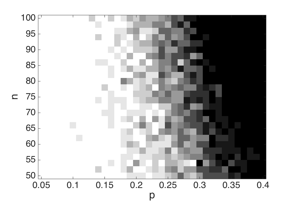
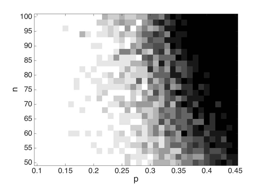
We investigate the performance of the Schur-Horn relaxation ( P ) in planted subgraph problems with the four planted subgraphs listed in Figure 6. For each of these graphs, we set equal to the eigenvalue corresponding to the largest eigenspace of the corresponding graph. We vary (the size of the larger graph inside which is planted) and (the probability of a noise edge in ), and we obtain random instances of planted subgraph problems for each value of and . In Figure 7, we plot the empirical probability of success of the Schur-Horn relaxation for these random trials; the white cells represent a probability of success of one and the black cells represent a probability of success of zero. Our results were obtained using the CVX parser [24, 25] and the SDPT3 solver [40]. In each of the four cases, the Schur-Horn relaxation ( P ) succeeds in solving the underlying planted subgraph problem for suitably small and .


5 Discussion
In this paper, we introduce a new convex relaxation approach for the planted subgraph problem, and we describe families of problem instances for which our method succeeds. Our method generalizes previous convex optimization techniques for identifying planted cliques based on nuclear norm minimization [2], and it is useful for identifying plangted subgraphs consisting of few distinct eigenvalues. There are several further directions that arise from our investigation, and we mention a few of these here.
Spectrally comonotone matrices with sparsity constraints
One of the ingredients in the proof of our main result Theorem 1 is to find a matrix that is spectrally comonotone with , and that further satisfies the condition that whenever . In the proof of Theorem 1 we simply choose . This choice does not exploit the fact that the entries of corresponding to those where are not constrained (and in particular can be nonzero). With a different choice of , one could replace in Theorem 1 by (recall that is an eigenspace of ). Consequently, our main result could be improved via principled constructions of matrices that satisfy the conditions of Theorem 1 and for which .
Sparse graphs with eigenspaces with large Kruskal rank
One of the central questions concerning the planted subgraph problem is the possibility of identifying ‘sparse’ planted subgraphs inside ‘dense’ noise via computationally tractable approaches. Concretely, suppose is a regular graph with degree . Under the Erdős-Rényi model for the noise, the average degree of any -node subgraph of the larger graph is about . From Theorem 1, we have that the Schur-Horn relaxation succeeds (with high probability) in identifying if , where is one of the eigenspaces of . In other words, (for suitably large ) if then the Schur-Horn relaxation succeeds in identifying inside despite the fact that is sparser than a typical -node subgraph in . Of the graphs we have investigated in this paper, the Clebsch graph from Figure 1(a) is an example in which both the degree and the Kruskal rank of the largest subspace are equal to . For some of the other small graphs discussed in this paper, the degree is larger than the Kruskal ranks of the eigenspaces. For larger graphs, the computation of the Kruskal rank of the large eigenspaces quickly becomes computationally intractable. Therefore, it is of interest to identify graph families in which (by construction) the degree is smaller than the Kruskal rank of one of the eigenspaces.
Convex geometry and graph theory
In developing convex relaxations for the planted subgraph problem (based on the formulation (1)) as well as other inverse problems involving unlabeled graphs, the key challenge is one of obtaining tractable convex outer approximations of the set for some given adjacency matrix . In particular, a convex approximation that contains is useful if the normal cone is large; as an example, the Schur-Horn relaxation has this property for adjacency matrices with few distinct eigenvalues. More generally, what is an appropriate convex relaxation for other structured graph families such as low-treewidth graphs (arising in inference in statistical graphical models), or graphs with a specified degree distribution (arising in social network analysis)? Recent work [13] provides a catalog of convex graph invariants that are useful for obtaining computationally tractable convex relaxations of . A deeper investigation of the interaction between convex-geometric aspects of these invariants (such as the normal cones of the associated convex relaxations) and the structural properties of the graph specified by the adjacency matrix has the potential to yield new convex relaxations for general inverse problems on graphs.
References
- [1] Noga Alon, Michael Krivelevich, and Benny Sudakov. Finding a large hidden clique in a random graph. Random Structures and Algorithms, 13(3-4):457–466, 1998.
- [2] Brendan P. W. Ames and Stephen A. Vavasis. Nuclear norm minimization for the planted clique and biclique problems. Mathematical Programming, 129(1):69–89, 2011.
- [3] Peter J. Artymiuk, Andrew R. Poirrette, Helen M. Grindley, David W. Rice, and Peter Willett. A graph-theoretic approach to the identification of three-dimensional patterns of amino acid side-chains in protein structures. Journal of Molecular Biology, 243(2):327–344, 1994.
- [4] Afonso S. Bandeira and Ramon van Handel. Sharp nonasymptotic bounds on the norm of random matrices with independent entries. Available online at arXiv:1408.6185 [math.PR], 2014.
- [5] Eiichi Bannai and Tatsuro Ito. Algebraic Combinatorics. Benjamin/Cummings, 1984.
- [6] Aharon Ben-Tal and Arkadi Nemirovski. Lectures on Modern Convex Optimization: Analysis, Algorithms, and Engineering Applications, volume 2. SIAM, 2001.
- [7] Raj C. Bose. Strongly regular graphs, partial geometries and partially balanced designs. Pacific Journal of Mathematics, 13(2):389–419, 1963.
- [8] W.G. Bridges and R.A. Mena. Multiplicative cones —- a family of three eigenvalue graphs. Aequationes Mathematicae, 22(1):208–214, 1981.
- [9] Andries E. Brouwer and Willem H. Haemers. Distance-regular graphs. Springer, 2012.
- [10] Andries E. Brouwer and Jacobus H. van Lint. Strongly regular graphs and partial geometries. Enumeration and Design, pages 85–122, 1984.
- [11] Peter J. Cameron. Strongly regular graphs. Selected Topics in Graph Theory, 1:pp–337, 1978.
- [12] Emmanuel J. Candès and Benjamin Recht. Exact matrix completion via convex optimization. Foundations of Computational Mathematics, 9(6):717–772, 2009.
- [13] Venkat Chandrasekaran, Pablo A. Parrilo, and Alan S. Willsky. Convex graph invariants. SIAM Review, 54(3):513–541, 2012.
- [14] Yaotsu Chang. Imprimitive symmetric association schemes of rank 4. PhD thesis, Thesis, University of Michigan, 1994.
- [15] Yichuan Ding and Henry Wolkowicz. A low-dimensional semidefinite relaxation for the quadratic assignment problem. Mathematics of Operations Research, 34(4):1008–1022, 2009.
- [16] Radu Dobrin, Qasim K. Beg, Albert-László Barabási, and Zoltán N. Oltvai. Aggregation of topological motifs in the escherichia coli transcriptional regulatory network. BMC Bioinformatics, 5(1):10, 2004.
- [17] David L. Donoho and Michael Elad. Optimally sparse representation in general (nonorthogonal) dictionaries via 1 minimization. Proceedings of the National Academy of Sciences, 100(5):2197–2202, 2003.
- [18] Michael Doob. Graphs with a small number of distinct eigenvalues. Annals of the New York Academy of Sciences, 175(1):104–110, 1970.
- [19] Michael Doob. On characterizing certain graphs with four eigenvalues by their spectra. Linear Algebra and its Applications, 3(4):461–482, 1970.
- [20] Maryam Fazel. Matrix rank minimization with applications. PhD thesis, Stanford University, 2002.
- [21] Uriel Feige and Robert Krauthgamer. Finding and certifying a large hidden clique in a semirandom graph. Random Structures and Algorithms, 16(2):195–208, 2000.
- [22] Gerd Finke, Rainer E. Burkard, and Franz Rendl. Quadratic assignment problems. Surveys in combinatorial optimization, 132:61, 2011.
- [23] Chris Godsil. Algebraic Combinatorics, volume 6. CRC Press, 1993.
- [24] Michael C. Grant and Stephen P. Boyd. CVX: Matlab software for disciplined convex programming.
- [25] Michael C. Grant and Stephen P. Boyd. Graph implementations for nonsmooth convex programs. In Recent Advances in Learning and Control, pages 95–110. Springer, 2008.
- [26] Willem H. Haemers and Vladimir D. Tonchev. Spreads in strongly regular graphs. Designs, Codes and Cryptography, 8(1-2):145–157, 1996.
- [27] Richard M. Karp. Reducibility among combinatorial problems. Springer, 1972.
- [28] Michael Krivelevich and Benny Sudakov. Pseudo-random graphs. In More Sets, Graphs and Numbers, pages 199–262. Springer, 2006.
- [29] Joseph B. Kruskal. Three-way arrays: rank and uniqueness of trilinear decompositions, with application to arithmetic complexity and statistics. Linear Algebra and Its Applications, 18(2):95–138, 1977.
- [30] Jure Leskovec, Kevin J. Lang, and Michael Mahoney. Empirical comparison of algorithms for network community detection. In Proceedings of the 19th international conference on World wide web, pages 631–640. ACM, 2010.
- [31] Oliver Mason and Mark Verwoerd. Graph theory and networks in biology. Systems Biology, IET, 1(2):89–119, 2007.
- [32] Rudolf Mathon. 3-class association schemes. In Proceedings of the Conference on Algebraic Aspects of Combinatorics, pages 123–155, 1975.
- [33] Nina Mishra, Robert Schreiber, Isabelle Stanton, and Robert E. Tarjan. Clustering social networks. In Algorithms and Models for the Web-Graph, pages 56–67. Springer, 2007.
- [34] Mikhail Muzychuk and Mikhail Klin. On graphs with three eigenvalues. Discrete Mathematics, 189(1):191–207, 1998.
- [35] Filippo Radicchi, Claudio Castellano, Federico Cecconi, Vittorio Loreto, and Domenico Parisi. Defining and identifying communities in networks. Proceedings of the National Academy of Sciences of the United States of America, 101(9):2658–2663, 2004.
- [36] Benjamin Recht, Maryam Fazel, and Pablo A. Parrilo. Guaranteed minimum-rank solutions of linear matrix equations via nuclear norm minimization. SIAM review, 52(3):471–501, 2010.
- [37] Ralph T. Rockafellar. Convex Analysis. Princeton University Press, 2015.
- [38] Raman Sanyal, Frank Sottile, and Bernd Sturmfels. Orbitopes. Mathematika, 57(02):275–314, 2011.
- [39] Johan J. Seidel. Strongly regular graphs. Recent Progress in Combinatorics, pages 185–198, 1969.
- [40] Kim-Chuan Toh, Michael J. Todd, and Reha H. Tütüncü. SDPT3 —- a matlab software package for semidefinite programming, version 1.3. Optimization Methods and Software, 11(1-4):545–581, 1999.
- [41] Edwin R. van Dam. Regular graphs with four eigenvalues. Linear Algebra and Its Applications, 226:139–162, 1995.
- [42] Edwin R. van Dam. Graphs with few eigenvalues. An interplay between combinatorics and algebra. PhD thesis, 1996.
- [43] Edwin R. van Dam and Edward Spence. Small regular graphs with four eigenvalues. Discrete Mathematics, 189(1):233–257, 1998.
- [44] Roman Vershynin. Introduction to the non-asymptotic analysis of random matrices. In Compressed Sensing, chapter 5, pages 210–268. Cambridge University Press, Cambridge, 2012.
- [45] John von Neumann. Some matrix inequalities and metrization of matrix space. Tomsk Univ. Rev, 1(11):286–300, 1937.