Secure and trusted white-box verification
Abstract
Verification is the process of checking whether a product has been implemented according to its prescribed specifications. We study the case of a designer (the developer) that needs to verify its design by a third party (the verifier), by making publicly available a limited amount of information about the design, namely a diagram of interconnections between the different design components, but not the components themselves or the intermediate values passed between components. We formalize this notion of limited information using tabular expressions as the description method for both the specifications and the design. Treating verification as a process akin to testing, we develop protocols that allow for the design to be verified on a set of inputs generated by the verifier, using any test-case generating algorithm that can take advantage of this extra available information (partially white-box testing), and without compromising the developer’s secret information. Our protocols work with both trusted and untrusted developers, and allow for the checking of the correctness of the verification process itself by any third party, and at any time.
1 Introduction
The following scenario is a rather common example of the design and development of a product: A car manufacturer needs to incorporate an engine component, made by a third subcontracting party, into its car design. In order to do that, it first produces the specifications of the component (described in a standard way), and announces them to the subcontractor. Then the latter implements its own design, and delivers the component, claiming that it complies with the specs. The car manufacturer, in turn, verifies that the claim is true, by running a set of test cases on the component, and confirming that the outputs produced for these test inputs are consistent with the specs. After the car design has been completed, a government agency needs to approve it, by running its own tests and confirming that the outputs comply with its own publicly-known set of environmental specs; once this happens, the car can be mass-produced and is allowed to be on the road. The only problem is that both the car manufacturer and the subcontractor do not want to reveal their designs to any third party, since they contain proprietary information, such as the setting of certain parameters that took years of experimentation to fine tune; therefore, and with only the specs publicly available, only black-box testing can be performed by the car manufacturer (vis-a-vis the subcontractor’s component), and the government agency (vis-a-vis the car). It may be the case, though, that the car manufacturer and/or the subcontractor are willing to reveal some partial information about their implementation(s) (possibly information that any good mechanic would figure out anyways given some time, such as which part is connected to some other part). In this case, an obvious question is the following: ”Can we allow for testing, that possibly takes advantage of this extra information, without revealing any information beyond that?” The answer to this question is rather obvious for the two extremes of (i) completely hidden information (only black-box testing is possible), and (ii) completely revealed information (completely white-box testing is possible). In this work, we present a method of answering the question in the affirmative in the continuum between these two extremes, i.e., for partially white-box testing.
More specifically, we are going to restrict our exposition to the case of Software Engineering, i.e., to software products, for clarity reasons, although our methods apply to any design whose specs and component interaction can be described using a standard description method, like tabular expressions [1]. There are two parties, i.e., a software developer (or product designer - we will use these terms interchangeably in what follows), and a verifier, as well as a publicly known set of specifications (or specs), also in a standard description. The two parties engage in a protocol, whose end-result must be the acceptance or rejection of the design by the verifier, and satisfies the following two properties:
- •
Correctness: If the two parties follow the protocol, and all test cases produced and tried by the verifier comply with the specs, then the verifier accepts, otherwise it rejects.
- •
Security: By following the protocol, the developer doesn’t reveal any bits of information in addition to the information that is publicly available.
In this setting, the specifications may come from the developer, the verifier, or a third party, but are always public knowledge. The algorithm that produces the test cases tried by the verifier is run by the latter, and is also publicly known and chosen ahead of time. Depending on the application, the developer may be either trusted (honest), i.e., follows the protocol exactly, providing always the correct (encrypted) replies to the verifier’s queries, or untrusted (dishonest) otherwise, and similarly for the verifier.
In this work, first we give a concrete notion of partial white-box testing, using tabular expressions as the description tool of choice. In its simpler form, a tabular expression is essentially a table with rows, with each row containing a left-hand side predicate on the table inputs, and a right-hand computation that produces the table outputs. The RHS of a row is executed iff the LHS predicate is evaluated to TRUE. A table describes the functionality of a design component; the description of the whole design is done by constructing a directed acyclic table graph, representing the interconnection of tables (nodes of the graph) as the output of one is used as an input to another (edges of the graph). Our crucial assumption is that the table graph is exactly the extra publicly-known information made available by the developer (in addition to the single publicly-known table describing the specifications); the contents of the tables-nodes, as well as the actual intermediate table input/output values should remain secret. Our goal is to facilitate the testing and compliance verification of designs that are comprised by many components, which may be off-the-shelf or implemented by third parties; if these components are trusted to comply with their specs by the developer (by, e.g., passing a similar verification process), then all the developer needs to know, in order to proceed with the verification of the whole design, is their input/output functionality, and not the particulars of their implementation. The formal definition of table graphs can be found in Section 2.1.
We present protocols that allow the verifier to run test case-generating algorithms that may take advantage of this extra available information (e.g., MC/DC [14]), and satisfy the correctness and security properties (formally defined in Section 2.3) with high probability (whp). We break the task of verification in a set of algorithms for the encryption of table contents and intermediate inputs/outputs (run by the developer), and an algorithm for checking the validity of the verification (cf. Definition 10); the former ensure the security property, while the latter will force the verifier to be honest, and allow any third party to verify the correctness of the verification process at any future time. Initially we present a protocol for the case of a trusted developer (Section 3), followed by a protocol for the case of a dishonest one (Section 4). Our main cryptographic tool is Fully Homomorphic Encryption (FHE), a powerful encryption concept that allows computation over encrypted data first implemented in [10]. We also employ bit-commitment protocols [20] in Section 4.
Previous work The goal of obfuscation, i.e., hiding the code of a program, while maintaining its original functionality, is very natural, and has been the focus of research for a long time. An obfuscated program reveals no information about the original program, other than what can be figured out by having black-box access to the original program. There are many heuristic obfuscation methods, e.g., [7], [29]. However, as shown in [3], an obfuscation algorithm that strictly satisfies the definition of obfuscation does not exist. Hence, all obfuscation algorithms can only achieve obfuscation to the extent of making obfuscated programs hard to reverse-engineer, while non black-box information about the original program cannot be guaranteed to be completely secret.
A crucial aspect of our work is the exclusion of any third-parties that act as authenticators, or guarantors, or a dedicated server controlled by both parties like the one in [5], called an ‘amanat’. In other words, we require that there is no shared resource between the two interacting parties, except the communication channel and the public specs. This reduces the opportunities for attacks (e.g., a malicious agent taking over a server, or a malicious guarantor), since they are reduced to attacking the channel, a very-well and studied problem.
Though ideal obfuscation is impossible to achieve, there are still some other cryptographic primitives that can be used to protect the content of a program. One is point function obfuscation [18], which allows for the obfuscation of a point function (i.e., a function that outputs 1 for one specific input, and 0 otherwise), but not arbitrary functions. Another relevant cryptographic primitive is Yao’s garbled circuits [31], which allow the computation of a circuit’s output on a given input, without revealing any information about the circuit or the input. Yao’s garbled circuits nearly achieve what obfuscation requires in terms of one-time usage, and are the foundation of work like one-time programs [13]. Its problem is that the circuit encryption (i.e., the garbled circuit) can be run only once without compromising security. Recently, [12] proposed a new version of garbled circuits called reusable garbled circuits, which allows for a many-time usage on the same garbled circuit, and still satisfies the security of Yao’s garbled circuits. [12] then uses reusable garbled circuits to implement token-based obfuscation, i.e., obfuscation that allows a program user to run the obfuscated program on any input, without having to ask the developer who obfuscated the program to encode the input before it is used. Token-based obfuscation guarantees that only black-box information about the original program can be figured out from the obfuscated program. Unfortunately, when a program is token-based obfuscated, it becomes a black box to the user (due to the inherent nature of obfuscation), and thus precludes its use for any kind of white-box verification. Building on [12], our work proposes a method to alleviate this weakness.
Plenty of work has been done in the field of verifiable computing, which is also relevant to our work. Verifiable computing allows one party (the prover) to generate the verifiable computation of a function, whose correctness a second party (a verifier - not related to the verifier in our setting) can then verify. For example, a naive way to do this, is to ask the verifier to repeat the computation of the function; however, in many cases this solution is both inefficient and incorrect. Recently, works like [8], [25], [28], [23], [24], [21], [4] which are based on the PCP theorem [2], presented systems that allow the verifier to verify the computation result without re-executing the function. The difference between verifiable computing and our work is that the developer wishes to hide the implementation of a design, while for verifiable computing, the design implementation cannot be hidden. However, verifiable computing still has the potential to be applied to the implementation of secure and trusted verification.
2 Preliminaries
2.1 Tabular Expressions (Tables)
Tabular expressions (or simply tables, as we are going to call them in this work) are used for the documentation of software programs (or, more generally, engineering designs). The concept was first introduced by David Parnas in the 1970s (cf. [1] and the references therein), and since then there has been a proliferation of different semantics and syntax variations developed. In this work we use a simple variation [30], already used in the development of critical software. Figure describes the structure of such a table. The Conditions column contains predicates , and the Functions column contains functions (constant values are regarded as zero-arity functions). The table works as follows: If for an input , then will be the output of table . To work properly, the predicates in must satisfy the disjointness and completeness properties:
- Completeness:
-
- Disjointness:
-
i.e., for any input exactly one of the table predicates is . Note that a table with a single row satisfies these properties only when . This is important, because we are going to work with an equivalent representation that has only single-row tables.
Condition Function


A table can be used to represent a module of a program (or a design). Then, the whole program can be documented as a directed graph with its different tables being the nodes of the graph, a source node Input representing the inputs to the program, and a sink node Output representing the outputs of the program. Every table is connected to the tables or Input where it gets its input from, and connecting to the tables or Output, depending on where its output is forwarded for further use. An example of such a graph can be seen in Figure . We will make the following common assumption (achieved, for example, by loop urolling) for table graphs:
Assumption 1.
The table graph of a program is acyclic.
2.1.1 Transformation to single-row tables
Our algorithms will work with single row tables. Therefore, we show how to transform the general tables and graph in Figure into an equivalent representation with one-row tables. The transformation is done in steps:
- •
As a first step, a table with rows is broken down into single-row tables. Note that, in general, the row of each multi-row table may receive different inputs and produce different outputs (with different destinations) that the other table rows; we keep the inputs and outputs of this row unchanged, when it becomes a separate table.
- •
We enhance each of the external input (introduced to the program at node Inputs, and transmitted through outgoing edges to the rest of the original table graph) with a special symbol , to produce a new input , with .
- •
Let be the (predicate, function) pair for the new (single-row) table, corresponding to an old row of an original table. As noticed above, , no matter what the input is. Let , where (i.e., the ’s are the ’s without the initial special symbol extension). The new function is defined as follows:
Note that and are special symbols, not related to the boolean values and . In particular, from now on, we will assume that in case the first part of a table output is , then this output will be recognized as a bogus argument, and will not be used as an input by a subsequent table. The reason for adding to ’s output will become apparent in Section 3.1.2.
After this transformation, we will get a transformed graph (Figure shows the transformed graph of the example in Figure ). From now on, by table graph we mean a transformed graph, by external input we mean an input that comes directly from Input, and by external output we mean an output that goes directly to Output. An intermediate input will be an input to a table that is the output of another table, and an intermediate output will be an output of a table that is used as an input to another table.
Since Assumption 1 holds, we can inductively order the tables of a table graph in levels as follows:
- •
An external input from node Input can be regarded as the output of a virtual level 0 table.
- •
A table is at level () if it has at least one incoming edge from a level table, and no incoming edges from tables of level larger than .
As a consequence, we can traverse a table graph (or subgraph) in an order of increasing levels; we call such a traversal consistent, because it allows for the correct evaluation of the graph tables (when evaluation is possible), starting from level . The graph structure of a table graph can be abstracted by a corresponding structure graph , which replaces each table in with a simple node. For example, Figure shows the structure graph for the table graph in Figure .
If is the set of tables in the representation of a program, we will use the shorthand
to denote that its transformed table graph contains both the table information of and the graph structure .
2.2 Cryptographic notation and definitions
We introduce some basic cryptographic notation and definitions that we are going to use, following the notation in [12]. We denote by a negligible function of K, i.e., a function such that for all , there exists with the property that . We use the notation p.p.t. as an abbreviation of probabilistic polynomial-time when referring to algorithms. Two ensembles and , where are probability distributions over for a polynomial , are computationally indistinguishable iff for every p.p.t. algorithm ,
We are going to use deterministic private key encryption (symmetric key encryption) schemes, defined as follows (see, e.g., [16]):
Definition 1 (Private key encryption scheme).
A private key encryption scheme is a tuple of three polynomial-time algorithms with the following properties:
- (1)
The key generation algorithm is a probabilistic algorithm that takes the security parameter as input, and outputs a key .
- (2)
The encryption algorithm is a deterministic algorithm that takes a key and a plaintext as input, and outputs a ciphertext .
- (3)
The decryption algorithm is a deterministic algorithm that takes as input a key and a ciphertext , and outputs the corresponding plaintext .
In order for an encryption to be considered secure, we require message indistinguishability, i.e., we require that an adversary must not be able to distinguish between two ciphertexts, even if it chooses the corresponding plaintexts itself. More formally:
Definition 2 (Single message indistinguishability).
A private key encryption scheme is single message indistinguishable iff for any security parameter K, for any two messages , and for any p.p.t. adversary ,
where the probabilities are taken over the (random) key produced by , and the coin tosses of .
An example of a private key encryption scheme satisfying Definitions 1 and 2 is the block cipher Data Encryption Standard (DES) in [9].
2.2.1 Fully Homomorphic Encryption (FHE)
We present the well-known definition of a powerful cryptographic primitive that we will use heavily in our protocols, namely the Fully Homomorphic Encryption (FHE) scheme (see [26] and [12] for the history of these schemes and references). This definition is built as the end-result of a sequence of definitions, which we give next:
Definition 3 (Homomorphic Encryption).
A homomorphic (public-key) encryption scheme is a tuple of four polynomial time algorithms with the following properties:
- (1)
is a probabilistic algorithm that takes as input a security parameter (in unary), and outputs a public key and a secret key .
- (2)
is a probabilistic algorithm that takes as input a public key and an input bit , and outputs a ciphertext .
- (3)
is a deterministic algorithm that takes as input a secret key and a ciphertext , and outputs a message bit.
- (4)
is a deterministic algorithm that takes as input the public key , a circuit with -bit input and a single-bit output, as well as ciphertexts . It outputs a ciphertext .
We will require that satisfies the compactness property: For all security parameters , there exists a polynomial such that for all input sizes , for all , and for all , the output length of is at most bits long.
Definition 4 (C-homomorphic scheme).
Let be a class of boolean circuits, where is a set of boolean circuits taking n bits as input. A scheme is C-homomorphic iff for every polynomial , sufficiently large , circuit , and input bit sequence , where , we have
| (1) |
where the probability is over the random bits of and .
Definition 5.
A scheme is fully homomorphic iff it is homomorphic for the class of all arithmetic circuits over .
Definition 6 (IND-CPA security).
A scheme HE is IND-CPA secure iff for any p.p.t. adversary A,
Fully homomorphic encryption has been a concept known for a long time, but it wasn’t until recently that Gentry [10] gave a feasible implementation of FHE. Our work is independent of particular FHE implementations; we only require their existence. For simplicity, sometimes we write when the public key isn’t needed explicitly. For an -bit string , we write instead of the concatenation , and we do the same for as well. Similarly, for with a circuit as its input such that outputs bits , sometimes we write to denote the concatenation .
We usually use to denote the ciphertext length of a one-bit FHE encryption.
Next, we present the multi-hop homomorphism definition of [11]. Multi-hop homomorphism is an important property for our algorithms, because it allows using the output of one homomorphic evaluation as an input to another homomorphic evaluation.
An ordered sequence of functions is compatible if the output length of is the same as the input length of , for all . The composition of these functions is denoted by . Given a procedure , we can define an extended procedure as follows: takes as input the public key , a compatible sequence , and a ciphertext . For , it sets , outputting the last ciphertext .
Definition 7 (Multi-hop homomorphic encryption scheme).
Let be a function of the security parameter . A scheme is an -hop homomorphic encryption scheme iff for every compatible sequence with functions, every input to , every (public,secret) key pair in the support of , and every in the support of ,
is a multi-hop homomorphic encryption scheme iff it is -hop for any polynomial .
2.2.2 Bit commitment protocols
Following Naor [20], a Commitment to Many Bits (CMB) protocol is defined as follows:
Definition 8 (Commitment to Many Bits (CMB) Protocol).
A CMB protocol consists of two stages:
- The commit stage:
-
Alice has a sequence of bits to which she wishes to commit to Bob. She and Bob enter a message exchange, and at the end of the stage Bob has some information about .
- The revealing stage:
-
Bob knows at the end of this stage.
The protocol must satisfy the following property for any p.p.t. Bob, for all polynomials , and for a large enough security parameter :
- •
For any two sequences and selected by Bob, following the commit stage Bob cannot guess whether Alice committed to or with probability greater than .
- •
Alice can reveal only one possible sequence of bits. If she tries to reveal a different sequence of bits, then she is caught with probability at least .
We are going to use the construction of a CMB protocol by Naor [20].
2.3 Evaluation and verification
Evaluation: Tabular expressions (tables) can be used to represent a program at different levels of abstraction. In this work, we concentrate on two levels: the specifications level, and the implementation level. Our goal is to design protocols that will allow a third party (usually called the verifier in our work) to securely and truthfully verify the compliance of a design at the implementation level (represented by a table graph ) with the publicly known specifications (represented by a table graph ), without publicly disclosing more than the structure graph of .
We are going to abuse notation, and use and also as functions , and . Wlog we assume that these two functions are over the same domain and have the same range, i.e., and .11 1 In general, the two pairs () and () may not be the same. Nevertheless, in this case there must be a predetermined mapping provided by the implementation designer, which converts () to () and vice versa, since, otherwise, the specifications verification is meaningless as a process.
The evaluation of (or any table graph), can be broken down into the evaluation of the individual tables level-by-level. The evaluation of a table at input produces an output . Note that some inputs may be null, if they come from non-evaluated tables, and if is not evaluated at all, then . In general, if some is or null, then we set .
Given an external input to the table graph , the evaluation of , is done as follows: Let be an ordering of the tables in in increasing level numbers (note that this is also a topological ordering, and that the first table is the virtual table of level ). Let be the tables that have external outputs. Then the evaluation of is the evaluation of its tables in the order, and is the set of the external outputs of . We call this process of evaluating consistent, because we will never try to evaluate a table with some input from a table that has not been already evaluated. All graph evaluations will be assumed to be consistent (otherwise they cannot be deterministically defined and then verified).
Verification: The verification processes we deal with here work in two phases:
- •
During the first phase, the table graph is analyzed, and a set of (external or internal) inputs is generated, using a publicly known verification test-case generation algorithm .
- •
In the second phase, and are evaluated on the set of inputs generated during the first phase. If the evaluations coincide, we say that passes the verification.
In our setting, is any algorithm that takes the publicly known as input, and outputs information that guides the verification (such as a set of external inputs to the table graph or certain paths of ). We emphasize that the output of is not necessarily external inputs. Our protocols can also work with any which generates enough information for the verifier to produce a corresponding set of external inputs, possibly by interacting with the designer of implementation . We also allow for verification on a (possibly empty) predetermined and publicly known set of pairs, i.e., for every with being a subset of the external inputs and a subset of external outputs, passes the verification iff can be evaluated and . The pairs in are called critical points.
Our protocols will use a security parameter , represented in unary as 1’s, i.e., as . Now, we are ready to define a trusted verifier (or trusted verification algorithm) (we use the two terms interchangeably):
Definition 9 (Trusted verifier).
A trusted verifier is a p.p.t. algorithm that uses random bits, and such that
where is a (possibly empty) set of external inputs generated by itself.
A verifier that satisfies Definition 9 is called trusted, because it behaves in the way a verifier is supposed to behave whp: Essentially, a trusted verifier uses the publicly known and a publicly known , to produce a set of external inputs ; it accepts iff the verification doesn’t fail at a point of or . During its running, the verifier can interact with the designer of . While is publicly known, the operations of the verifier are straight-forward, even without any interaction with the designer. The problem in our case is that the verifier has only an encryption of , and yet, it needs to evaluate in order to perform its test. This paper shows how to succeed in doing that, interacting with the designer of , and without leaking more information about than the publicly known .
In what follows, a verifier will be a part of a verification scheme, generally defined as follows:
Definition 10 (Verification scheme).
A verification scheme is a tuple of p.p.t. algorithms such that
- •
is a p.p.t. algorithm that takes a security parameter and a table graph as input, and outputs an encrypted table graph .
- •
is a p.p.t. algorithm that takes an input and returns an encoding .
- •
is a p.p.t. algorithm that takes a security parameter and a public as input, has an honest verifier satisfying Definition 9 hardcoded in it, and outputs if the verification has been done correctly (and otherwise).
From now on, it will be assumed (by the verifier and the general public) that the encryption by the designer is done (or looks like it has been done) by using a publicly known algorithm (with a secret key, of course). If the designer’s encryptions don’t comply with the format of ’s output, the verification fails automatically.
In general, it may be the case that an algorithm claiming to be a trusted verifier within a verification scheme, doesn’t satisfy Definition 9 (either maliciously or unintentionally). Such a malicious verifier may claim that a design passes or doesn’t pass the verification process, when the opposite is true. In order to guard against such a behaviour, we will require that there is a piece of public information, that will act as a certificate, and will allow the exact replication of the verification process by any other verifier and at any (possibly later) time; if this other verifier is a known trusted verifier, it will detect an incorrect verification with high probability (whp). We emphasize that the interaction (i.e., the messages exchange) shown in Figure 3 is done publicly. In fact, we will use the transaction record as a certificate (cf. Definition 10), that can be used to replicate and check the verification, as described above.
Hence, we will require that our verification schemes are:
- •
secure, i.e., they don’t leak the designer’s private information, and
- •
correct, i.e., they produce the correct verification result whp.
More formally, we define:
Definition 11 (Correctness).
A verification scheme is correct iff the following holds: if and only if both of the following hold:
| (2) | |||
| (3) |
where is the honest verifier hardwired in , and is the table graph produced by .
Condition (3) forces to be trusted, and condition (2) ensures that its verification is correct whp, even when applied to instead of ; together ensure the correctness of the verification whp.
Just as it is done in [12], we give a standard definition of security:
Definition 12 (Security).
For any two pairs of p.p.t. algorithms and , consider the two experiments in Figure 2.
| 1. |
| 2. |
| 3. |
| 4. Output |
| 1. |
| 2. |
| 3. |
| 4. Output |
A verification scheme is secure iff there exist a pair of p.p.t. algorithms (simulators) , and an oracle such that for all pairs of p.p.t. adversaries , the following is true for any p.p.t. algorithm :
i.e., the two experiments are computationally indistinguishable.
Definition 13 (Secure and trusted verification scheme).

Remark 1.
and in Step 3 of the two experiments in Figure 2 are not oracles used by . In these experiments, plays the role of a (potentially malicious) verifier and interacts with the developer as shown in Figure 3. More specifically, in , picks an input , asks the developer to run (instead of querying an oracle), and receives the answer. In , again asks the developer, but, unlike , the latter runs instead of and provides with the answer. Hence, whenever we say that queries or , we mean that asks the developer to run or respectively, and provide the answer. Note that is an oracle queried by .
In what follows, first we deal (in Section 3) with an honest designer/developer, i.e., a developer that answers honestly the verifier’s queries:
Definition 14.
An honest developer is a developer that calls to generate in Figure 3, when queried by the verifier.
3 Secure and trusted verification for honest developers
3.1 Construction outline
In this section, we construct a secure verification scheme satisfying Definition 13. In a nutshell, we are looking for a scheme that, given an encrypted table graph and its structure graph, will verify the correctness of evaluation on a set of test external inputs, in a secure way; to ensure the latter, we will require that the intermediate table inputs/outputs produced during the verification process are also encrypted.
3.1.1 VS.Encrypt
In order to encrypt the rhs functions of the tables as well as the intermediate inputs/outputs, we use universal circuits [27]. If we represent each function in (transformed) table as a boolean circuit (see Appendix A for methods to do this), then we construct a universal circuit and a string for each , so that for any input , . Following [22] (a method also used in [12]), and can be encrypted, while the computation can still be performed and output an encryption of .
Therefore, fully homomorphically encrypts with FHE’s public key to get , and replaces each table with its encrypted version . Then, if a verifier wants to evaluate at , it gets the FHE encryption of , and runs to get . Because holds, we have that . Note that the encrypted graph that outputs maintains the same structure graph as the original table graph , and that outputs in addition to . Algorithm 1 implements .
3.1.2 VS.Encode
is going to address two cases:
- 1.
Suppose the verifier is evaluating an encrypted table whose output is an external output. From the construction of , we know that its output is an FHE-encrypted ciphertext. But the verifier needs the plaintext of this ciphertext in order for verification to work. We certainly cannot allow the verifier itself to decrypt this ciphertext, because then the verifier (knowing the secret key of the encryption) would be able to decrypt the encrypted circuit inside as well. What we can do is to allow the verifier to ask the developer for the plaintext; then the latter calls to decrypt this ciphertext for the verifier.
- 2.
Suppose the verifier is evaluating an encrypted table whose output is an internal output used as an input to another table. In this case, we cannot allow the verifier to simply ask the developer to decrypt this output as before; that would give away the intermediate outputs, which are supposed to be kept secret. At the same time, the verifier must be able to figure out whether the actual (unencrypted) value of this intermediate output is or not, i.e., “meaningful” or not. More specifically, should be able to tell whether intermediate output contains or . (Recall from Section 2 that an original table in outputs a symbol if the predicate in the initial table graph is not satisfied, i.e., ’s output is not “meaningful”.)
In Case 2, particular care must be taken when the verifier chooses an external input for table . The verifier is required to use the FHE encryption of in order to evaluate . An obvious way to do this is to let the verifier compute , and evaluate
However, this simple solution can be attacked by a malicious verifier as follows: The verifier chooses one of the intermediate outputs, and claims that this intermediate output is the encryption of the external input. Then Case 1 applies, and the verifier asks the developer for the output of . Then it is obvious that through this interaction with the developer, the verifier can extract some partial information about the intermediate output. We use to prevent this malicious behaviour: For any external input chosen by the verifier, the latter cannot fully homomorphically encrypt the input by itself; instead, it must send the input to the developer, who, in turn, generates the FHE encryption by calling .
In order to allow to distinguish between the two cases, we introduce an extra input parameter that takes a value from the set of special ’symbols’ meaning the following:
- :
-
is called with . Index indicates the th table and is an external input to (Case 1).
- :
-
is called with . Index indicates the th table and is an intermediate input to (Case 2).
Also, we allow to store data in a memory , which is wiped clean only at the beginning of the protocol. Algorithm 2 implements .
3.1.3 VS.Eval
is an algorithm that allows anyone to check whether the verification was done correctly. In order to achieve this, the interaction between the verifier and the developer is recorded in a public file . By reading , can infer which inputs and tables the verifier evaluates, and what outputs it gets. This allows to evaluate the tables on the same inputs, using its own verifier, and at any time, and check whether the outputs are the recorded ones. Obviously, by using only an honest verifier and , essentially checks whether the verifier that interacted with the developer originally was also honest.
More specifically, takes input , and outputs or (i.e., accept or reject the verification, respectively). The record file records a sequence of (verifier query, developer reply) pairs , where is the verifier query, and is the reply generated by the developer when it runs (the last pair obviously records the verifier’s output). It also records test-generator , the set of critical points used, and the random seed used by to produce the test points. Finally, it records the encrypted table graph , the public FHE key , and the universal circuit . As mentioned above, the pairs are public knowledge. Algorithm 3 implements . is the hardwired honest verifier.
3.1.4 VS.Path
We can provide the verifier with the ability to choose and evaluate paths in . The verifier picks a path in the table graph, passes it to the developer, and the latter runs in order to generate an external input that, when used, will lead to the evaluation of the tables on the path chosen by the verifier. Algorithm 3 implements .
3.1.5 Encrypted table graph evaluation
The evaluation of an encrypted table graph is more complex than the evaluation of an unencrypted table graph . The evaluation of at an external input (i.e., ) is done by Algorithm 5.
3.2 Correctness and security
We have described an implementation of , , of Definition 10. Note that plays the role of for . In this section we prove the compliance of our scheme with Definitions 11 and 12. Recall that is the fully homomorphic encryption scheme introduced in Section 2.2.1.
3.2.1 Correctness
Proof.
We will need the following lemma:
Lemma 1.
When outputs , for any table and , the output claimed by as must be equal to , i.e., evaluates every table correctly.
Proof.
Given that the verifier used by is an honest one, the lemma is obviously true. ∎
For the the (query,answer) pairs in that do not belong to a consistent traversal of , Algorithm 2 (lines 11, 12, 14, 17) will return as the corresponding input encodings, and Algorithm 5 (lines 9, 14) will compute for tables with such inputs. Therefore, security and correctness are not an issue in this case. From now, on we will concentrate on the consistent table traversals and their inputs/outputs.
Lemma 2.
Given the external input set , common to both and , for any table with input and output , there is a corresponding table and input , such that
| (4) |
where is the public key generated by .
Proof.
We prove this lemma by induction on the level of a table.
Base case: Level tables have only external inputs, and, therefore, Algorithm 2 (line 5) returns . Also, from line 22 of Algorithm 5 we have
Inductive step: Suppose that for any table whose level is smaller than and its input , table and its input satisfy (4). Then we show that for any level table with input , the level table and its encoded input satisfy (4).
For any , either for some , or is an external input. In case is external, then satisfies (4) like in the base case. Otherwise, is a table of level smaller than . Then, because of the inductive hypothesis,
(The last equation is valid because encrypts a string bit by bit.)
Now, the second part of (4) is proven similarly to the base case. ∎
Lemma 3.
The input-output functionality of is the same as the input-output functionality of .
Proof.
Lemma 2 (and hence Lemma 3) are based on the verifier evaluating every table correctly and its subgraph traversal being consistent. Assuming that the traversal is indeed consistent (something easy to check on ), by running , we can know whether satisfies Lemma 1 ( outputs ). If this is the case, we know that ’s evaluation of has the same result as the evaluation of with the same inputs, i.e., (2) in Definition 11 holds. Moreover, if outputs , (3) in Definition 11 also holds (see lines 6 - 12 in Algorithm 3). ∎
3.2.2 Security
Following the approach of [12], we prove the following
Proof.
In Definition 12 the two simulators and simulate and respectively. In our implementation we have added , so we add to simulate , together with its own oracle . We can think of as a combination that plays the role of , and as a combination that plays the role of in of Figure 2: depending on the kind of query posed by , replies if it is an ”Encode” query, and replies if it is a ”Path” query. The tuple of simulators which satisfies Definition 13 is constructed as follows:
- •
runs in two steps:
- Step 1:
-
generates its own table graph with its own tables .
- Step 2:
-
runs (Algorithm 1) and obtains .
- •
receives queries from the of Definition 12, and can query its oracle (described in Algorithm 6). actually simulates , passing the queries from to its -like oracle . has a state (or memory) which is initially empty, and contains the mapping of the encrypted table output to the real table output for a given query. returns the outputs of as the answers to the queries of .
- •
simulates . It receives queries from , and queries its oracle (described in Algorithm 7) in turn. Then returns the output of to .
First, we construct an experiment (see Figure 4), which is slightly different to in Definition 12. In , the queries of are not answered by calls to and , but, instead, they are answered by calls to and (recall that and together are the simulator ). We use the shorthands and for and in respectively.
| : |
|---|
| 1. |
| 2. |
| 3. |
| 4. Output |
Lemma 4.
Experiments and are computationally indistinguishable.
Proof.
First, note that and have the same functionality (see Algorithms 4 and 7). We prove that and have the same input-output functionality. By the construction of (see lines 1 - 7 in Algorithm 2) and (see lines 1 - 7 in Algorithm 6), when a query is of the form , both algorithms will output the FHE encryption of , so they have the same input-output functionality. The case of a query is more complex; there are two cases:
Case 1: Algorithm 2 outputs . This happens in the following cases:
- 1.
An intermediate input which should be the output of , is not ’s output (see line 11).
- 2.
An intermediate input is the output of a , but ’s output is (see line 12).
- 3.
The FHE encryption of an external input cannot be found in ’s memory , where it should have been if it had already been processed (as it should) by (see line 14).
- 4.
(see line 17).
These four cases will also cause Algorithm 6 to output in lines 10-14 (for the first and second), lines 15 - 18 (for the third), and line 21 (for the fourth).
Case 2: Algorithm 2 doesn’t output . Suppose is the external input to and is the input to . There are three cases for (see lines 19 - 23 in Algorithm 2):
- 1.
If ’s output is an intermediate output and the FHE encryption of , then decrypts , and outputs .
- 2.
If ’s output is an intermediate output and not the FHE encryption of , then decrypts , and outputs .
- 3.
If ’s output is an external output, then decrypts , and outputs the second component of (i.e., the actual output).
On the other hand, when calculates at (the unencrypted ) in lines 8 - 24 of Algorithm 6, there are three cases (see lines 25 - 26 in Algorithm 6):
- 1.
If ’s output is an intermediate output and is , the output is .
- 2.
If ’s output is an intermediate output and is not , the output is .
- 3.
If ’s output is an external output, the output is the second component of .
The first two cases are the same for and . In the third case, Algorithm 2 outputs the second half of , while Algorithm 6 outputs the second component of , which are the same because of (4). Therefore, and have the same input-output functionality. ∎
In order to prove Theorem 2, we first prove the security of a single table:
Lemma 5.
For every p.p.t. adversary , and any table , consider the following two experiments:
| 1. | . |
| 2. | |
| 3. | Let be a circuit that computes ’s function. |
| 4. | Generate universal circuit and string , such that . |
| 5. | |
| 6. | |
| 7. | Output |
| 1. | . |
| 2. | |
| 3. | Let be produced by Step 1 of |
| 4. | Construct circuit that computes the function of . |
| 5. | Generate universal circuit and string , such that |
| 6. | |
| 7. | |
| 8. | Output |
The outputs of the two experiments are computationally indistinguishable.
Proof.
If ’s inputs in and are computationally indistinguishable, then ’s outputs are also computationally indistinguishable. The former is true, because and are two FHE ciphertexts, and, therefore, they are computationally indistinguishable under the IND-CPA security of FHE. ∎
We generate a sequence of different table graphs, each differing with its predecessor and successor only at one table:
All these new table graphs have the same structure graph . To each corresponds the experiment in Figure 6.
| 1. | |
| 2. | |
| 3. | Generate universal circuit |
| 4. | For |
| • Construct with an -bit output and computes the function of . | |
| • Generate string such that . | |
| • | |
| 5. | Let be produced by Step 1 of |
| 6. | For |
| • Construct circuit computing the function of . | |
| • Generate string such that . | |
| • | |
| 7. | |
| 8. | |
| 9. | Output |
Note that is the same experiment as , since Step 5 is the first step of and Steps 2,3,6,7 are doing exactly what the second step of does (i.e., ). Also note that is the same as in Figure 4, since the part of is ignored, and is the results of , i.e., .
Now we are ready to prove that is computationally indistinguishable from by contradiction. Assume that and are computationally distinguishable, and, therefore, and are computationally distinguishable, i.e., there is a pair of p.p.t. adversaries and a p.p.t. algorithm such that
| (5) |
Since
inequality (5) implies that there exists such that
We use to construct a pair of p.p.t. algorithms which together with p.p.t. algorithm contradict Lemma 5, by distinguishing to . Specifically, they determine whether Step 6 of or Step 7 of has been executed. can distinguish the two experiments, if it can distinguish between its two potential inputs and . The idea is to extend the table or (whichever the case) into a full table graph or (whichever the case), appropriate for experiments or (whichever the case), and invoke which can distinguish between the two. is described in Figure 7, where the table graph is either or . Hence, by the construction of , we know that can be used to distinguish between experiments and for .
| 1. | |
| 2. | Construct a circuit , and a string such that |
| 3. | |
| 4. | |
| 5. | Output |
| 1. | For |
| • Construct circuit that computes the function of . ( comes from ) | |
| • Generate string such that . | |
| • | |
| • Construct table | |
| 2. | Construct just as does. |
| 3. | For |
| • Construct circuit that computes the function of | |
| • Generate string such that . | |
| • | |
| • Construct table | |
| 4. | |
| 5. |
∎
Theorem 3.
Our verification scheme satisfies Definition 13.
4 Secure and trusted verification for general developers
In general, the developer may not comply with Definition 14, i.e., the developer can actually replace with some other malicious algorithm in its interaction with the verifier. If we do not provide a method to prevent this scenario from happening, then a buggy implementation could pass the verifier’s verification when it actually should not.
Bearing this in mind, we replace our old definition of a verification scheme with a new one in Definition 15 below, by adding an algorithm , which the verifier can ask the developer to run in order to determine whether the latter indeed runs . itself is also run by the developer, which immediately poses the danger of being replaced by some other algorithm . Therefore, must be designed so that even if it is replaced by some other algorithm, the verifier can still figure out that the developer doesn’t run or from its replies.
In the new extended definition, , , and remain the same. By running with a publicly known , any third party can check whether the developer is malicious and whether the verification was done correctly.
Definition 15 (Extension of Definition 10).
A verification scheme is a tuple of p.p.t. algorithms such that
- •
is a p.p.t. algorithm that takes a security parameter and a table graph as input, and outputs an encrypted table graph .
- •
is a p.p.t. algorithm that takes an input and returns an encoding .
- •
is a p.p.t. algorithm that takes a security parameter and a public as input, has an honest verifier satisfying Definition 9 hardcoded in it, and outputs if the verification has been done correctly (and otherwise).
- •
is a p.p.t. algorithm with a memory that receives a question from the verifier and replies with an answer , so that the verifier can detect whether the developer indeed runs and .
Figure 8 shows what should be a round of the protocol between the developer and the verifier.

Definition 16 (Correctness).
A verification scheme is correct iff the following holds: if and only if all of the following hold:
| (6) | |||
| (7) | |||
| (8) |
where is the verifier hardwired in , and is the table graph produced by .
Definition 17 (Security).
For and which are tuples of p.p.t algorithms, consider the two experiments in Figure 9.
| 1. |
| 2. |
| 3. |
| 4. Output |
| 1. |
| 2. |
| 3. |
| 4. Output |
A verification scheme is secure if there exist a tuple of p.p.t. simulators and oracles such that for all pairs of p.p.t. adversaries , the following is true for any p.p.t. algorithm :
i.e., the two experiments are computationally indistinguishable.
Correspondingly, we update Definition 13:
Definition 18 (Secure and trusted verification scheme).
The updated Definition 14 becomes
Definition 19.
A developer is honest iff it always runs and . Otherwise it is called malicious.
Remark 2.
, , and in Step 3 of the two experiments in Figure 9 are not oracles used by . In these experiments, plays the role of a (potentially malicious) verifier and interacts with the developer as shown in Figure 8. More specifically, in , asks the developer to run or on inputs of its choice (instead of querying an oracle), and receives the answer. In , again asks the developer, but, unlike , the latter runs instead of and instead of , and provides with the answer. Hence, whenever we say that queries , , or we mean that asks the developer to run , , or respectively, and provide the answer. Note that are oracles for respectively.
We repeat that in Section 3 we required that the developer satisfied Definition 12, but that developer may not comply with Definition 19 in this section.
4.1 Construction outline
, and are exactly the same as in Section 3.
4.1.1 VS.Checker
In order to illustrate how is going to be used, we use Figure 10 as an example of the evaluation of a table graph (on the left) and its encrypted version (on the right).

There are three potential points where a developer can tinker with , namely, when the verifier is querying for an external output (bottom application of in Figure 10), for an intermediate output (middle application of in Figure 10), and for an external input (top application of in Figure 10).
Case 1: External output. We start with this case, since it is somewhat more straight-forward; so, for now, we will assume that the developer has indeed run in the previous tables of the path. Suppose asks the developer to run to decrypt the external output of table in Figure 10. The correct output of should be the external output , but a malicious developer can replace with a which outputs . can use the following method to detect this behaviour:
- Step 1
-
Ahead of running the protocol, announces the use of a deterministic private key encryption scheme (see Definition 1), and chooses a secret key . (’s encryption algorithm is , represented in a circuit format compatible with .)
- Step 2
-
first extracts the second component of , which is , and then runs ,,, to get a result .
- Step 3
-
sends to the developer and asks it to run in order to fully homomorphically decrypt ; the developer returns ’s output , which we denote as .
- Step 4
-
uses ’s decryption algorithm to decrypt and get .
- Step 5
-
compares with the (known) external output . If they are the same, knows that the developer indeed run , otherwise knows that the developer is malicious.
Obviously, if the developer decides to run , i.e., , it gets which it returns to . Then obtains by evaluating , and compares it with the answer from the developer who is expected to run . If they are not the same, rejects. Now suppose that the developer runs some instead of , sending a value , and some , sending a value . Then uses its secret key to decrypt and gets , which is not whp, leading to rejecting whp.
Case 2: Intermediate output. Again, assuming (for now) that the developer has indeed run in the previous tables of the path in Figure 10, this is the case of getting the intermediate output . What is allowed to know from the developer is whether this intermediate output is meaningful or not, namely, whether contains or (cf. Section 3.1). A malicious developer can run instead of and return instead of . The method for described in Case 1 can also be used here by changing Step 2, so that first extracts the first half of (which is ), and then runs to get .
Case 3: External input. This is the case of an external input (see top of Figure 10). The verifier can treat this case exactly like Case 1, to confirm that is actually a fully homomorphic encryption of .
By doing a consistent traversal of , and applying the relevant Case 1-3 each time (i.e., starting with external inputs (Case 3) and working its way through finally the external outputs (Case 1)), can enforce the developer to run (and ) in all steps. Unfortunately, allowing to ask the developer to run actually makes far more powerful, and there is a risk that may abuse this power, by sending queries with malicious content to . Therefore we need to force into asking the ‘right’ queries. For example, in Step 3 of Case 1, must check whether before it decrypts . Our solution to this problem is to use a bit commitment protocol during the interaction between the verifier and the developer. A description of the interaction between developer and verifier during the execution of such a protocol can be found in Appendix B. Algorithm 8 implements . The definition of is exactly the same as in Section 3.1.
4.1.2 VS.Eval
is an extension of in Section 3.1.3. It not only needs to check whether the verifier evaluates the table graph correctly, but it also needs to check whether the developer replies honestly. In order to check whether the verifier evaluates the table graph correctly, runs Algorithm 3. In addition, by reading the log file which records the interaction between the verifier and the developer, can check whether the verifier actually asks the developer to run for every answer it gets (allegedly) from . Actually, can recreate the whole interaction between the verifier and the developer from this log file.
The log file is (as before) but extended with an extra set which contains tuples ; each such tuple contains a query by to , the information generated by both the developer and the verifier during the bit commitment protocol, and the answer returned by the developer after running . Hence, for each record generated, a record will also be generated.
Algorithm 9 implements , taking logs as its input.
4.2 Correctness and security
In our implementation, the used by in Definition 15 is . In Definition 17, simulators , and simulate , and respectively. Similarly to Section 3.2, we add one more simulator to simulate , and its corresponding oracle (Algorithm 7). Algorithm 10 describes the oracle used by to simulate .
4.2.1 Correctness
We show the following
Theorem 4.
The verification scheme introduced in this section satisfies Definition 16.
Proof.
Lemma 6.
If , then (7) holds.
Proof.
Suppose that and . For brevity reasons, we will only consider the case of , and is an external output. The other cases ( or is not an external output), are similar. Also, since the bit commitment protocol succeeds whp, can be assumed to be honest.
First we consider the case of and having the same input-output functionality. Let be the tuple that corresponds to the current query . Suppose that outputs a value , while would output . If , then we know (see line 18 in Algorithm 9)
| (9) |
Therefore, to prove that , it is enough to prove that
| (10) |
According to ’s construction (see lines 8-9 in Algorithm 8),
| (11) |
where . Since and have the same input-output functionality, given as input to both and , their outputs are the same, i.e., , where is the output of and is the output of . According to the construction of (see lines 19-23 in Algorithm 2) ,
| (12) |
Therefore,
| (13) |
On the other hand, whp Definition 4 implies that
| (14) |
Hence, by combining (11) and (14) we get
which implies that
| (15) |
Next we consider the case of and having the same input-output functionality. For , and the corresponding pair , is the input of and its output, while is the input of and its output. Since , we know that (9) holds (see line 18 in Algorithm 9). Also (12) is obviously true, as is (11) (see lines 8-9 in Algorithm 8). The latter, together with the identical functionality of , implies that
| (16) |
Hence, by combining (9),(16),(14) we have
Hence, (13) holds, and combined with (13) and (12), we get , i.e., given as input to and , their outputs are the same whp.
Finally suppose that there exists and corresponding such that and . We know (see lines 19-23 in Algorithm 2) that (12) holds, and, by combining (11), (12) and (14), we get
Since and , and do not satisfy (9) whp. But according to ’s construction (see line 18 in Algorithm 9), when , (9) holds whp, a contradiction. ∎
Proof.
∎
4.2.2 Security
Following the methodology of [12], we will show the following
Theorem 5.
The verification scheme VS introduced in this section satisfies Definition 17.
Proof.
We construct a tuple of simulators so that , and are the same as in the proof of Theorem 2. receives queries from , queries oracle (Algorithm 10), and returns the output of to .
In our proof, we will need to define a new experiment (cf. Figure 11).
| 1. | |
| 2. | |
| 3. | |
| 4. | Output |
and (cf. Figure 9) differ only in Step 3, where queries in and in . If we can show that and have the same input-output functionality, then and are computationally indistinguishable.
To prove this we distinguish two cases for an input to and .
First, when outputs , it is easy to see that will also output ; this happens when the size of or is not correct (line 1 in Algorithm 8 and 5 in Algorithm 10), when is not generated by the evaluation of a table or (line 5 in Algorithm 8 and line 14 in Algorithm 10), and when the bit commitment protocol fails (lines 11-20 in Algorithm 8 and lines 14-23 in Algorithm 10).
Second, when does not output , it will output a value ; in this case first generates the same (see lines 8-12 of Algorithm 10), and after passing the bit commitment protocol, it also outputs .
Therefore and have the same input-output functionality. Hence and are computationally indistinguishable:
| (17) |
and in Figure 12 are the experiments and in Definition 12, with added to and added to (see Figure 2).
| 1. |
| 2. |
| 3. |
| 4. Output |
| 1. |
| 2. |
| 3. |
| 4. Output |
In the same way as in Theorem 2, we can show that and are computationally indistinguishable, i.e., for all pairs of p.p.t. adversaries and any p.p.t. algorithm ,
| (18) |
Assume that and are computationally distinguishable. Then (17) implies that and are computationally distinguishable, i.e., there are a p.p.t. algorithm and a p.p.t. adversary such that
| (19) |
A p.p.t. adversary that wants to distinguish between and can use and as follows:
- •
runs and outputs .
- •
gets one of the two:
- –
and has oracle access to , or
- –
and has oracle access to
depending on which one of the two experiments ( and ) is executed. Then constructs and (which are also used in and ), and runs providing it with access to . Its output will be either or , depending again on which of and is being executed.
- –
If is being executed, then it can easily be seen that
If is being executed, then it can easily be seen that
But then, (19) implies that
which contradicts (18). Therefore, and are computationally indistinguishable. ∎
5 Open problems
We have presented protocols that implement secure and trusted verification of a design, taking advantage of any extra information about the structure of the design component interconnections that may be available. Although we show the feasibility of such verification schemes, ours is but a first step, that leaves many questions open for future research.
- •
Improving efficiency Our implementation uses FHE, which, up to the present, has been rather far from being implemented in a computationally efficient way. On the other hand, garbled circuits are usually considered to be more efficient than FHE schemes; for example, [15] shows that garbled circuits were much more efficient than a homomorphic encryption scheme in certain Hamming distance computations. Therefore, pursuing protocols based on Yao’s garbled circuits is a worthy goal, even if a more efficient garbled circuits construction is less secure.
- •
Verifiable computing Although verifiable computing is not yet applicable to our case (as mentioned in the Introduction), coming up with a method to hide the computation would provide a more efficient solution to the problem of secure and trusted verification, since the amount of re-computation of results needed would be significantly reduced.
- •
Hiding the graph structure Our work has been based on the assumption that the table graph of a design is known. But even this may be a piece of information that the designer is unwilling to provide, since it could still leak some information about the design. For example, suppose that the design uses an off-the-shelf subdesign whose component structure is publicly known; then, by looking for this subgraph inside , someone can figure out whether this subdesign has been used or not. In this case, methods of hiding the graph structure, by, e.g., node anonymization such as in [32], [6], may be possible to be combined with our or other methods, to provide more security.
- •
Public information vs. testing The extra information we require in order to allow some white-box test case generation by the verifier, namely the table graph structure, is tailored on specific testing algorithms (such as MC/DC [14]), which produce computation paths in that graph. But since there are other possibilities for test case generation, the obvious problem is to identify the partial information needed for applying these test generation algorithms, and the development of protocols for secure and trusted verification in these cases.
References
- [1] T. A. Alspaugh, S. R. Faulk, K. H. Britton, R. A. Parker, and D. L. Parnas. Software requirements for the A-7E aircraft. Technical report, DTIC Document, 1992.
- [2] S. Arora and S. Safra. Probabilistic checking of proofs: A new characterization of NP. Journal of the ACM (JACM), 45(1):70–122, 1998.
- [3] B. Barak, O. Goldreich, R. Impagliazzo, S. Rudich, A. Sahai, S. Vadhan, and K. Yang. On the (im)possibility of obfuscating programs. In CRYPTO 2001, pages 1–18. Springer, 2001.
- [4] E. Ben-Sasson, A. Chiesa, D. Genkin, E. Tromer, and M. Virza. SNARKs for C: Verifying program executions succinctly and in zero knowledge. In Proceedings of CRYPTO 2013, pages 90–108. Springer, 2013.
- [5] S. Chaki, C. Schallhart, and H. Veith. Verification across intellectual property boundaries. ACM Trans. on Software Eng. and Methodology (TOSEM), 22, 2013.
- [6] J. Cheng, A. W. Fu, and J. Liu. K-isomorphism: privacy preserving network publication against structural attacks. In Proceedings of the 2010 ACM SIGMOD International Conference on Management of data, pages 459–470. ACM, 2010.
- [7] C. Collberg, C. Thomborson, and D. Low. A taxonomy of obfuscating transformations. Technical report, Department of Computer Science, The University of Auckland, New Zealand, 1997.
- [8] G. Cormode, M. Mitzenmacher, and J. Thaler. Practical verified computation with streaming interactive proofs. In Proceedings of the 3rd Innovations in Theoretical Computer Science Conference, pages 90–112. ACM, 2012.
- [9] FIPS. Data Encryption Standard. NBS, 46, January 1977.
- [10] C. Gentry. A fully homomorphic encryption scheme. PhD thesis, Stanford University, 2009.
- [11] C. Gentry, S. Halevi, and V. Vaikuntanathan. -hop homomorphic encryption and rerandomizable Yao circuits. In Proceedings of CRYPTO 2010, pages 155–172. Springer, 2010.
- [12] S. Goldwasser, Y. Kalai, R. A. Popa, V. Vaikuntanathan, and N. Zeldovich. Reusable garbled circuits and succinct functional encryption. In Proceedings of the 45th ACM Symposium on Theory Of Computing (STOC), pages 555–564. ACM, 2013.
- [13] S. Goldwasser, Yael Tauman Kalai, and Guy N Rothblum. One-time programs. In CRYPTO 2008, pages 39–56. Springer, 2008.
- [14] K. J. Hayhurst, D. S. Veerhusen, J. J. Chilenski, and L. K. Rierson. A practical tutorial on modified condition/decision coverage. Technical Report TM-2001-210876, NASA, 2001.
- [15] Y. Huang, D. Evans, J. Katz, and L. Malka. Faster secure two-party computation using garbled circuits. In Proceedings of the 20th USENIX conference on Security SEC’11, pages 35–35, 2011.
- [16] J. Katz and Y. Lindell. Introduction to modern cryptography. CRC Press, 2014.
- [17] J. Kilian. Uses of randomness in algorithms and protocols. PhD thesis, MIT, 1989.
- [18] B. Lynn, M. Prabhakaran, and A. Sahai. Positive results and techniques for obfuscation. In EUROCRYPT 2004, pages 20–39. Springer, 2004.
- [19] D. Malkhi, N. Nisan, B. Pinkas, and Y. Sella. Fairplay- a secure two-party computation system. In Proceedings of the 13th conference on USENIX Security Symposium SSYM’04, volume 13, pages 20–20, 2004.
- [20] M. Naor. Bit commitment using pseudorandomness. Journal of Cryptology, 4(2):151–158, 1991.
- [21] B. Parno, J. Howell, C. Gentry, and M. Raykova. Pinocchio: Nearly practical verifiable computation. In Proceedings of the 2013 IEEE Symposium on Security and Privacy (SP), pages 238–252. IEEE, 2013.
- [22] T. Sander, A. Young, and M. Yung. Non-interactive cryptocomputing for NC1. In Proceedings of the 40th Annual Symposium on Foundations of Computer Science (FOCS), pages 554–566. IEEE, 1999.
- [23] S. Setty, R. McPherson, A. J. Blumberg, and M. Walfish. Making argument systems for outsourced computation practical (sometimes). In Proceedings of the 19th Annual Network & Distributed System Security Symposium, 2012.
- [24] S. Setty, V. Vu, N. Panpalia, B. Braun, A. J. Blumberg, and M. Walfish. Taking proof-based verified computation a few steps closer to practicality. In Proceedings of the 21st USENIX conference on Security symposium, Security’12, pages 253–268, 2012.
- [25] J. Thaler, M. Roberts, M. Mitzenmacher, and H. Pfister. Verifiable computation with massively parallel interactive proofs. In Proceedings of the 4th USENIX conference on Hot Topics in Cloud Computing, HotCloud’12, 2012.
- [26] V. Vaikuntanathan. Computing blindfolded: New developments in fully homomorphic encryption. In Proceedings of the 52nd IEEE Annual Symposium on Foundations of Computer Science (FOCS), pages 5–16. IEEE, 2011.
- [27] L. G. Valiant. Universal circuits (preliminary report). In Proceedings of the 8th annual ACM Symposium on Theory Of Computing (STOC), pages 196–203. ACM, 1976.
- [28] V. Vu, S. Setty, A. J. Blumberg, and M. Walfish. A hybrid architecture for interactive verifiable computation. In Proceeding of the 2013 IEEE Symposium on Security and Privacy, SP’13, pages 223–237. IEEE, 2013.
- [29] C. Wang, J. Hill, J. Knight, and J. Davidson. Software tamper resistance: Obstructing static analysis of programs. Technical Report CS-2000-12, University of Virginia, 2000.
- [30] A. Wassyng and R. Janicki. Tabular expressions in software engineering. Fundamenta Informaticae, 67:343–370, 2005.
- [31] A. C. Yao. Protocols for secure computations. In Proceedings of the 54th IEEE Annual Symposium on Foundations of Computer Science (FOCS), pages 160–164. IEEE, 1982.
- [32] B. Zhou and J. Pei. Preserving privacy in social networks against neighborhood attacks. In Proceedings of the 24th IEEE International Conference on Data Engineering, ICDE’08, pages 506–515. IEEE, 2008.
Appendix A Conversion of functions to circuits
We have mentioned above that in our construction the rhs functions in the tables of a table graph will be converted into boolean circuits in order for our construction to work properly. But we did not say how the conversion is done or whether this conversion is practical. Essentially what our construction requires is an automatic way to transform a higher level description of a function into a boolean circuit. Transformation of a higher level description of a function into a lower level description like a circuit was done in [19], [15]. [19] introduces a system called FAIRPLAY which includes a high level language SFDL that is similar to C and Pascal. FAIRPLAY allows the developer to describe the function in SFDL, and automatically compiles it into a description of a boolean circuit. A similar system is described in [15], and is claimed to be faster and more practical than FAIRPLAY. This system allows the developer to design a function directly in Java, and automatically compiles it into a description of a boolean circuit.
Appendix B Bit commitment protocols
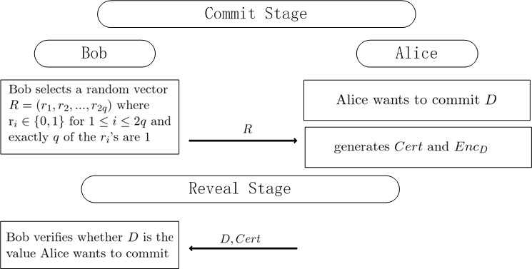
We are going to use the construction of a CMB protocol by Naor [20].
Let be a code of words, such that the Hamming distance between any is at least , for some . Let be an efficiently computable encoding function that maps to . It is also required that and , where is a fixed constant.
denotes a pseudo-random generator :, such that for all p.p.t. adversary A ,
where the probabilities are taken over and seed chosen uniformly at random.
denotes the first bits of the pseudo-random sequence on seed and denotes the th bit of the pseudo-random sequence on seed .
For a vector with and indices such that , denotes the vector where and is the index of the th 1 in . If , then denotes the bitwise Xor of and .
Suppose Alice commits to .
- •
Commit Stage:
- 1.
Bob selects a random vector where for and exactly of the ’s are 1, and sends it to Alice.
- 2.
Alice computes , selects a seed and sends to Bob which is the following: Alice sends Bob (the bitwise Xor of and ), and for each such that she sends .
- 1.
- •
Reveal Stage: Alice sends s and . Bob verifies that for all such that , Alice has sent the correct , computes and , and verifies that .
We denote by , the bits by , the seed by ; a schematic diagram of the protocol can be found in Figure 13.
B.1 Use of BCP in Section 4.1
The idea of a bit commitment protocol is similar to hiding information in an envelope [17]. The developer runs which does the following: First, given an input , fully homomorphically decrypts and gets a value . The developer puts in a sealed envelope and gives it to . cannot open the envelope at this stage. After that, needs to provide a proof that is indeed . The proof contains the secret key , but revealing to does not matter, because ’s output is already given to and cannot change at this point. If confirms that is indeed , then it generates a key to the sealed envelope, and the developer gives this key to . Then can know , using the key to open the envelope. If figures out that is not , it simply refuses to generate the key to the envelope. Such an envelope solves the problem of mutual distrust and potential malicious activities by both entities. A bit commitment protocol can play the role of such an envelope.
Appendix C The protocol of Section 3

Appendix D An example for Section 3
In this subsection we use an example in Figure 15 to show how to apply our verification scheme to actually verify a specific table graph. In Figure 15 there is an initial table graph that is to be verified by the verifier .

First the developer transforms this initial table graph into a table graph introduced in Section 2.2 (see Figure 1c). Then
The developer applies our content-secure verification scheme to . It runs as follows. . Figure 16 is the encrypted table graph .

According to our protocol, the verifier receives and does the verification on . We show how can do MC/DC verification [14] on . MC/DC performs structural coverage analysis. First it gets test cases generated from analysing a given program’s requirements. Then it checks whether these test cases actually covers the given program’s structure and finds out the part of the program’s structure which is not covered. First we assume the that uses will do MC/DC verification after it generates the test cases. Suppose runs to generate the test cases, based on requirements-based tests (by analysing ), and these test cases are stored in EI. Then picks an external input to from and starts evaluating with .
For , sends the following queries to the developer (The queries are in the format of the input of ): , , , , , , because it needs to evaluate , , , , , as well as an encoding for the external inputs of each table. We take the evaluation of the path (Input Output) as an example. For query , evaluates and returns ( is the output of ), which is the input to . Then runs and outputs . After this sends to . Because we know that for , if 46 is the input to , then the output will be . Thus for the query , evaluates and returns . Hence knows that for a=46 as an external input, the lhs predicate (a decision and condition) of is satisfied, and the rhs function of is covered.
After finishing evaluating , starts evaluating and with as their input. is ’s input. After finishing evaluating , gets as the output. Then sends to . evaluates and ’s output is (Because , ’s output is . We also know that the output of is an external output. Accordingly, outputs ). Therefore, returns to . Then knows that as well as the fact that the lhs predicate (a decision and condition) of is satisfied and the rhs function of is covered.
After evaluating with by similar steps as described above and getting the external output , knows that for , the lhs predicates of , and are satisfied while the rest tables’ lhs predicates are not satisfied. Hence, knows that the predicates of , and are while the predicates in the rest tables of are and the statements (the rhs functions of the tables in ) of , and are covered. Moreover, compares with to see if behaves as expected with as an external input.
will keep evaluating with the rest external inputs in , and by interacting with in the way as described above, it does the structural coverage analysis of the requirements-based test cases. He will be able to know whether the external inputs in covers every predicates in . Additionally, it will be able to know whether behaves as expected in the requirements specification described by .
Appendix E The protocol of Section 4
