A Nonparametric Likelihood Approach for Inference in Instrumental Variable Models
Abstract
Instrumental variable methods allow for inference about the treatment effect by controlling for unmeasured confounding in randomized experiments with noncompliance. However, many studies do not consider the observed compliance behavior in the testing procedure, which can lead to a loss of power. In this paper, we propose a novel nonparametric likelihood approach, referred to as the binomial likelihood method, that incorporates information on compliance behavior while overcoming several limitations of previous techniques and utilizing the advantages of likelihood methods. Our proposed method produces proper estimates of the counterfactual distribution functions by maximizing the binomial likelihood over the space of distribution functions. Using this we propose two versions of a binomial likelihood ratio test for the null hypothesis of no treatment effect. We show that both versions are more powerful to detect any distributional change than existing methods in finite sample cases, and are asymptotically equivalent to the two-sample Anderson-Darling test. We also develop an efficient algorithm for computing our estimates, and apply the binomial likelihood method to a study of the effect of Medicaid coverage on mental health using the Oregon Health Insurance Experiment.
1 Introduction
The instrumental variables (IV) method is a popular technique for estimating the casual effect of a treatment in the presence of unmeasured confounding (Angrist et al.,, 1996; Tan,, 2006; Baiocchi et al.,, 2014). This arises in situations where, even through direct randomization is impossible, an encouragement to take the treatment can be randomized (Holland,, 1988), or there is a “natural experiment” such that some people are encouraged to receive the treatment compared to others in a way that is effectively random (Angrist et al.,, 1996). Informally, an instrument is a variable that affects the treatment but is independent of unmeasured confounders and only affects the outcome through affecting the treatment (see Section 2.1 for a more precise definition). Under a monotonicity assumption that the encouraging level of the instrument never causes someone not to take the treatment, the treatment effect can be identified for the compliers, those subjects who would take the treatment if they were encouraged to take the treatment but would not take the treatment if they were not encouraged (see Angrist et al., (1996), Abadie, (2003), Baiocchi et al., (2014), Brookhart and Schneeweiss, (2007), Cheng et al., 2009a (), Cheng et al., 2009b (), Hernan and Robins, (2006), Kang et al., (2018), Johnson et al., (2019), Ogburn et al., (2015), Tan, (2006) and the references therein for methods of inference using instrumental variables).
In causal inference, to evaluate the treatment effect on the outcome, Fisher’s sharp hypothesis of no effect is often considered, which, in the potential outcome framework (Neyman,, 1923; Rubin,, 1974), asserts that the two potential outcomes and , which are the outcomes individual would experience with or without treatment, respectively, are the same for every individual . Under the IV assumptions, where the treatment effect can be identified for the compliers, the hypothesis of no effect for compliers can be tested by comparing the distributions of and for compliers. Unfortunately, it is difficult to make inference about these distributions since researchers do not know who are the compliers from data. Abadie, (2002) proposed an approach that indirectly compares the two potential outcome distributions, by using the Kolmogorov–Smirnov test statistic. However, this approach ignores the treatment variable during the testing procedure. Thus, it does not consider the compliance class information of the individuals, which can lead to loss of power, as discussed in Rubin, (1998).
In this paper, we propose a novel nonparametric likelihood-based approach for comparing the two counterfactual distribution functions, with or without treatment for compliers, that uses the compliance class information and allows for estimation and hypothesis testing in a common holistic framework. This requires a methodological innovation because the usual nonparametric likelihood approach using the empirical likelihood (Owen,, 2001) does not work for the IV model because there are infinitely many solutions that maximize the likelihood (Geman and Hwang,, 1982). Our proposed binomial likelihood (BL) approach creates a piece of likelihood at each knot (or evaluating point), by using binomially distributed outcomes: outcomes smaller than or equal to the knot, and outcomes larger than the knot. Then, it multiplies together the pieces of these likelihoods across all knots creating a composite likelihood. This is a “pseudo” likelihood rather than the true likelihood because the binomial random variables are actually dependent, but are treated as independent in the composite likelihood. Due to its binomial nature in defining likelihood functions, we specifically call this composite likelihood, the binomial likelihood (BL). Composite likelihood has been found useful in a range of areas including problems in geostatistics, spatial extremes, space-time models, clustered data, longitudinal data, time series and statistical genetics; see Lindsay, (1988), Heagerty and Lele, (1998), Larribe and Fearnhead, (2011), and Varin et al., (2011).
The BL approach can be used for statistical inference similar to the usual likelihood method. For instance, for estimating the distribution functions of the compliers, the maximum binomial likelihood (MBL) estimate can be obtained by maximizing the BL over the space of distribution functions. Therefore, by definition, the MBL estimates satisfy the necessary conditions for a proper distribution function (increasing and non-negative). This make the BL estimates easily interpretable, and is a major improvement over the naive plug-in estimates, which can be non-monotonic and negative. As a consequence, the BL method can be effectively used for making further inferences, such as integrating utility functions or estimating moments of the probability function. Furthermore, similar to classical likelihood ratio tests, the binomial likelihood ratio test (BLRT) for the null hypothesis of no treatment effect can be constructed by taking the ratio of two BL values that are maximized over the null and the alternative respectively. For computing the MBL estimate and conducting hypothesis testing using the BLRT we develop a computationally efficient iterative algorithm based on the expectation-maximization (EM) and pool-adjacent-violators (PAV) algorithms. Thus, the BL approach provides the practitioners with a comprehensive toolbox for causal inference in non-parametric IV problems.
The BL method has several attractive limiting and finite-sample properties. To begin with, we show that the MBL estimate for the distribution function of the compliers has the same first-order asymptotics (limiting distribution) as the naive plug-in estimates. This shows that the BL estimates, which preserve all the properties of a proper distribution, have no loss in asymptotic efficiency compared to the naive estimates, which can be non-monotone and negative in finite samples. For hypothesis testing, we show that the BLRT is asymptotically equivalent to the well-known Anderson–Darling two-sample test (Pettitt,, 1976). Since there are no closed form expressions for the BL estimates in general, these asymptotic results are important to the understanding of the BL approach. The BLRT also has better finite-sample performance for detecting distributional changes compared to other baseline methods. The improvement is especially significant in the weak IV setting, exhibiting the importance of incorporating the compliance class information for hypothesis testing in IV models. We also apply the BL approach to study the effect of Medicaid coverage for African American adults on self-reported mental health, as studied by Baicker et al., (2013).
The rest of the article is organized as follows. Basic notation and assumptions of the IV model are discussed in Section 2. In this section, we also review the existing plug-in approach for testing the hypothesis of no effect. In Section 3, we introduce the BL approach and derive the asymptotic properties of the MBL estimate (Theorem 1). In Section 4, we develop two versions of the BLRT for testing the null hypothesis, and derive the asymptotic properties of the tests (Theorems 2 and 3). In Section 5 we discuss the algorithm for computing the BL estimates and present the numerical results for the BLRT. The analysis of the real data is given in Section 6. Proofs of the theorems and additional simulations are given in the supplementary materials.
2 Framework and Review
2.1 Assumptions and Identification with Instrumental Variables
For individual , denote as the binary IV, as the indicator variable for whether individual receives the treatment or not, and as the outcome variable that is continuous in this paper. Using the potential outcome framework (Neyman,, 1923; Rubin,, 1974), define as the value that would be if were to be set to 0, and as the value that would be if were to be set to 1. Similarly, for , is the value that the outcome would be if and . For each individual , the analyst can only observe one of the two potential values and , and one of the four potential values . The observed treatment is Similarly, the observed outcome can be expressed as . An individual’s compliance class is determined by the combination of the potential treatment values and , which is denoted by : always-taker (at) if ; never-taker (nt) if ; complier (co) if ; and defier (de) if .
For the rest of this paper, the following standard identifying conditions are assumed. The implications of these conditions are briefly explained in the paragraph below; see Angrist et al., (1996) for more details on these conditions.
Assumption 1.
The following identification conditions will be imposed on the instrumental variable model:
- (a)
Stable Unit Treatment Value Assumption (SUTVA) (Rubin,, 1986): The outcome (treatment) for individual is not affected by the values of the treatment or instrument (instrument) for other individuals and the outcome (treatment) does not depend on the way the treatment or instrument (instrument) is administered.
- (b)
The instrumental variable is independent of the potential outcomes and potential treatment .
- (c)
Nonzero average causal effect of on : .
- (d)
Monotonicity: .
- (e)
Exclusion restriction: , for or .
Assumption 1 enables the causal effect of the treatment for the subpopulation of the compliers to be identified. Condition (a) allows us to use the notation (or ), which means that the outcome (treatment) for individual is not affected by the values of the treatment and instrument (instrument) for other individuals. Condition (b) will be satisfied if is randomized. Condition (c) requires to have some effect on the average probability of treatment. Condition (d), the monotonicity assumption, means that the possibility of , is excluded, that is, there are no defiers. Condition (e) assures that any effect of on must be through an effect of on . Under this assumption, the potential outcome can be written as , instead of .
Let , . Also, let , and be the cumulative distribution functions of the outcome for compliers without treatment, never-takers, compliers with treatment, and always-takers respectively. For and , under Assumption 1, they are identified as the distributions of the potential outcome and respectively, for example, . Similarly, we define the distribution functions of corresponding to combinations of . Denote . Although can be more accurate notation than since and are conditioned on, we will instead use simpler notation . Any notation involving followed by a subscript means the distribution function of conditioning on the subscript. Also, we define the probabilities for . Finally, let , be the mixture distribution of . The outcomes are independent and identically distributed from . Under Assumption 1, as discussed in Abadie, (2002), both and can be identified as
| (1) |
Also, and can be identified under Assumption 1 as and .
2.2 Testing Fisher’s Null Hypothesis of No Effect: Review of the Existing Approaches
A central question in causal inference is to understand if the treatment has any causal effect on the outcome. To evaluate the treatment effect on the outcome, Fisher’s sharp hypothesis of no effect can be considered. Under Assumption 1, it can be tested whether there is any causal treatment effect for compliers. Technically, Fisher’s hypothesis can be constructed for compliers as for . However, cannot be directly tested since only one of the two potential outcomes for each individual can be observed. Instead, we consider a test for equality of distributions using the potential outcome distributions for compliers,
| (2) |
The existing approach for testing is based on the fact that implies where under Assumption 1. Abadie, (2002) proposed using the Kolmogorov–Smirnov test , where are the empirical distribution functions for . This test is the comparison between the outcome distribution of the group and the outcome distribution of the group. To show a connection between these two distributions with the compliers’ distribution functions and , define the plug-in estimates obtained using (1) as
| (3) |
where , , , , and are the empirical distribution functions, . Since , is equivalent to the test based on comparison between and . However, the plug-in estimates have two limitations: (1) violating the non-decreasing condition of distribution functions and (2) being unstable when an IV is weak. First, the violation leads to producing estimates that are often located outside of . Therefore, they are not proper estimates of and , which is due to not incorporating the observed information on compliance behavior. Furthermore, the test statistic can be unusually large if is small, which occurs when an IV is weak. As discussed in Rubin, (1998), making use of the IV structure can produce a better test statistic, and thus increase power.
To employ the structure of the instrumental variable model, one simple way is to transform the plug-in estimates to proper distribution functions by using the monotone rearrangement method (Chernozhukov et al.,, 2010), followed by truncation to . Chernozhukov et al., (2010) showed that the transformed estimates have the same first-order properties (asymptotic distribution) as the plug-in estimates. The rearrangement method produces a quick fix of the plug-in estimates and provides promising empirical properties, however it is difficult to use the method in hypothesis testing for evaluating the asymptotic properties.
Remark 1.
The plug-in estimators and are obtained as (3). Other plug-in estimators are and . We denote the vector of the plug-in estimators of the outcome distribution functions, as . We consider the plug-in estimators of the compliance classes as a function of such that where and for all with terminology slightly abused.
3 The Binomial Likelihood (BL) Approach
3.1 Constructing Binomial Likelihood with An Instrumental Variable
Define such that =, , , where , , , : are functional variables representing four different outcome distributions. Instead of using previously defined , we use the parameter set to emphasize the fact that it is a variable to be estimated. Similarly, we can define the parameter such that , where and are functional variables representing the proportions of compliance classes. Since the true proportions and do not depend on knots, we take the average across the knots to build estimators for them. We set knots that are the locations to evaluate BL functions later. Then, and are the estimators of and respectively. Also, we define , and then is the estimator of . Furthermore, we use that is the estimator of . Finally, we define that is the estimator of . For example, , , and .
Denote the data where , , . Also, denote the event . The probability can be easily computed in terms of the variables . At each knot , we define the point-knot-specific BL function for a data point ,
Then, by aggregating the point-knot-specific BL functions across all data points, we can define the knot-specific BL function at knot ,
Finally, we can define the BL function by taking the geometric mean of the knot-specific BL functions across all knots,
| (4) |
The BL function depends on the choice of knots even when the data points are fixed. The knots can be given by researchers, but we propose to use all observed outcomes as knots. More specifically, we use the order statistics as knots with . This selection procedure provides an automatic way to build the BL function and avoids an arbitrary decision that may cause a favorable conclusion. The contributions of the knot-specific BL functions are, obviously, not independent on data points. Nevertheless, we pretend they are independent. To reduce such dependency, a random sample from can be chosen as knots in practice. Also, for a large , the size of knots does not need to be . A smaller set of knots can be helpful for reducing computation time. Although we choose , we emphasize that, for general knots , the BL function can be constructed and also the MBL estimator can be obtained. Theoretical results in the following section are derived for knots . As long as the distribution of knots is the same as the distribution of , the theoretical arguments hold.
Remark 2.
The knot-specific BL function at knot for some becomes zero when any of is either 0 or 1. This occasionally occurs at the extreme order statistics. To avoid technicalities in the proofs arising from this, we define the likelihood function (4) over the central order statistics, that is, for for a small fixed constant . Throughout the proofs in the supplementary materials, the asymptotics will be in the regime where the sample size grows to infinity, keeping fixed. We omit dependence on in the BL for notational brevity. Also, in practice, to avoid computational issues, we can let the knot-specific BL values be 1 when probabilities vanish on the boundary.
3.2 The Maximum Binomial Likelihood (MBL) Method
In Section 3.1, we introduce a BL approach for constructing a nonparametric likelihood function. Given the BL function , we propose the maximum binomial likelihood (MBL) method to obtain the estimates of by maximizing them over their parameters spaces. To this end, denote as the space of all distribution functions from . Let , and be the parameter spaces for and .
Definition 1.
The MBL estimate is defined as
| (5) |
where and are defined at the knots .
Remark 3.
The complete parameter space of the three parameters will be hereafter referred to as the restricted parameter space. To ensure that (5) is well-defined, we extend between the knots by using coordinate-wise right-continuous interpolation and extrapolation beyond the knots by 0 or 1. Also, and are the estimators of and .
The full expression of the binomial log-likelihood function is long and unwieldy. However, we can rewrite it in a compact and instructive form, by grouping and rearranging the terms. It follows (see proof of Proposition 1 below for details) that , where , and
with , for , defined as follows:
where the function .
Proposition 1.
Let be the binomial likelihood estimates as defined in (5). Then that is equal to the plug-in estimate , and
Proof.
See Section A in the Supplementary Material. ∎
This proposition shows that the MBL estimate of is the proportion of individuals with instrument (that is, ) in the observed sample. Furthermore, the MBL estimates of and can be obtained by maximizing the function .
Remark 4.
Maximizing the BL function over the unrestricted parameter space , where with the set of all functions from and , produces the plug-in estimates (see Lemma 1 in the Supplementary Material for the proof).
3.3 Asymptotic Properties of The MBL Estimates
In this section we discuss the asymptotic properties of the MBL estimates , and how they compare with the plug-in estimates . Assume the knots , for .
Assumption 2.
We assume the following:
- (a)
The proportion parameter vector belongs to the interior of the parameter space .
- (b)
The distribution functions are continuous, strictly increasing, and have the same support.
- (c)
For all compact, , there exists constants (depending on ) such that .
In particular, Assumption 2 holds whenever are differentiable and the derivatives are uniformly bounded above and below, that is, , for all , and compact. Under this assumption we show that the MBL estimates and the plug-in estimates have mean squared errors converging to zero, after rescaling by . Recall that is the true population outcome distribution of .
Theorem 1.
For any fixed , let and . Then, the MBL estimates and the plug-in estimates satisfy
and
| (6) |
where the term goes to zero as . Moreover, . Also, it implies that the two estimators and of the population for satisfy
Proof.
See Section B in the Supplementary Material. ∎
The theorem shows that and (also, and ) have the same first-order behavior, and hence the same limiting distribution, which can be derived using the Brownian bridge approximation of the empirical distribution functions; see Corollary 1 (Section C) in the Supplementary Material. Interestingly, Chernozhukov et al., (2010) showed the monotone rearrangement estimates also have the same first-order behavior as the plug-in estimates, which together with Theorem 1, implies that the MBL estimates have the same first-order properties as the rearrangement estimates.
Remark 5.
The proof of Theorem 1 can be easily modified to show finite dimensional convergence, that is, for every and given , . This would imply that the finite dimensional distributions of the plug-in estimate process and the MBL estimate process are asymptotically the same. We present this result in terms of mean squared errors as in (6), because it emerges naturally from the asymptotic properties of the BL function, and can be directly applied to the analysis of the BLRT that is introduced in Section 4.
4 Extension of the BL Approach: Hypothesis Testing
4.1 Binomial Likelihood Ratio Test (BLRT): Full Version
The BL approach can be extended to constructing a likelihood ratio-type test in a similar way that the ML approach can be extended to constructing a likelihood ratio test. We take two times the difference in two binomial log-likelihood values; one is obtained with the constraint (that is, under the null) and the other is obtained without this constraint (that is, under the alternative). This gives a new test for the null hypothesis , and hereafter, we call it the binomial likelihood ratio test (BLRT).
Define the restricted null parameter space as , where is the set of distribution functions from . Then, the BLRT statistic is obtained by
| (7) |
Let . The asymptotic properties of can be derived as we did for in Theorem 1. Also, we can derive the asymptotically equivalent plugin-type estimators that have not been studied before. It is worth noting that the explicit form of the equivalent estimators of is provided in Section D, the Supplementary Material.
Theorem 2.
Fix and recall that . Let be the binomial likelihood ratio test statistic as defined in (7). Denote . Then,
where is the empirical distribution function of .
Proof.
See Section E in the Supplementary Material. ∎
This theorem gives an asymptotically equivalent representation of the BLRT statistic as the two-sample Anderson-Darling test statistic (Pettitt,, 1976). It can be used to construct the rejection region and compute the critical value for a given significance level. Moreover, this shows that the test based on is consistent against all fixed alternatives, because of the universal consistency of the two-sample Anderson-Darling test (Scholz and Stephens,, 1987).
However, in finite-sample settings, the critical value obtained from the asymptotic distribution of can be conservative. In the theorem above, to derive the asymptotic properties, we use the equivalent plug-in estimators of instead of using directly. However, they do not lie in the restricted parameter space, which leads to a gap between the equivalent and actual BL values. This gap fades out as increases, but it can be critical when we evaluate finite-sample performance. This issue will be further discussed in the simulation section.
The BLRT is developed for testing the null hypothesis that assumes no treatment effect for compliers. The BLRT can be further extended to testing other hypotheses like for some . To test , a simple modification is required. A new outcome variable can be generated: if , and otherwise. Then, can be used for the BLRT as (7), and this test based on the new dataset conducts a hypothesis test for . Among many choices of , can be considered to check whether there is any location shift between the two distributions. The assumption of the location shift means that there is a constant treatment effect for all compliers. Therefore, this test can be used for examining treatment effect heterogeneity. If is rejected for all , then there is evidence that treatment effects are heterogeneous.
4.2 Binomial Likelihood Ratio Test: Simple Version
As we discussed in section 2.2, under Assumption 1, testing the null hypothesis is equivalent to testing the null hypothesis . Based on this, we propose a simple version of the BLRT by comparing instead of . This test does not use the information of compliance classes by ignoring the treatment , but uses only and . We define the parameter such that , where are functional variables representing the outcome distributions for and . Then, given that is conditioned on, the simple version binomial log-likelihood function is
| (8) |
where . The simple version BLRT statistic is defined as
Since this test does not use any information of the compliance class behaviors, it does not require estimation of the proportions, and estimation of the outcome distribution for the compliance classes. The following gives the asymptotic approximation of .
Theorem 3.
The test statistic has an explicit form as
If we assume that the knots are , then the test statistic is asymptotically equivalent to the two-sample Anderson-Darling test statistic, that is,
Proof.
See Section E in the Supplementary Material. ∎
Theorem 3 shows that, as in the case of the full version BLRT, the simple version BLRT is asymptotically equivalent to the two-sample Anderson-Darling test, and, therefore, is consistent against all fixed alternatives, as well. The difference is that has a closed form and does not need the EM-PAV algorithm that will be introduced in the next section. However, does not involve any estimation procedure of outcome distributions for compliance classes, and, hence, cannot be applied for estimation purposes.
5 Computation and Simulation
5.1 EM-PAV Algorithm for Computing the MBL Estimates
There are no closed form solutions to the MBL estimates. However, the estimates can be computed efficiently by using a combination of the expectation-maximization (EM) algorithm and the pool-adjacent-violator(PAV) algorithm. We call it the EM-PAV algorithm. To begin with, we introduce the complete-data , which includes the compliance class , . If and are known, then is determined; for example, if and , then . Denote the event , where .
Given the complete data, we can define a point-knot-specific complete-data binomial likelihood function for the data point at knot ,
The complete-data binomial likelihood is obtained by combining all point-knot-specific complete-data likelihood functions in the same way to define the BL,
As in the BL, the dependence on in the complete-data likelihood is separable, that is,
where , and does not depend on . Hereafter, we will refer to as the complete-data binomial log-likelihood. To find the maximizer of , our algorithm is initiated by specifying the initial values that lie in the parameter space . Then the following steps are repeated until the values converge:
Algorithm 1.
(EM-PAV algorithm) Let and be the outputs after the th step of the iteration. The following shows the th step.
(Expectation Step) Given these outputs and the observed data , the expected complete-data binomial log-likelihood is
The expectation can be easily calculated; see Section F2 in the Supplementary Material for computational details.
(Maximization Step) To begin with, define
Note that where is evaluated at knots , and similarly for other estimates. Observe that is the unrestricted maximizer of . These estimates can be computed explicitly; see Section F3 in the Supplementary Material. It can be shown that is actually in the restricted space , that is, and for any knot . Define . In general, however, , because may not satisfy the non-decreasing condition of distribution functions. To ensure the monotonicity constraint we apply the PAV algorithm to the estimate ,
where the operation PAVw is applied coordinate-wise and the weight vector is , where the weights are defined in Section F in the Supplementary Material.
The following proposition establishes the correctness of this algorithm.
Proposition 2.
Let be as defined above. Then
Proof.
See Section F in the Supplementary Material. ∎
5.2 Simulation: Performance of BLRT
| vs. | |||||||
| IV | (boot.) | (asymp.) | |||||
|---|---|---|---|---|---|---|---|
| Strong | 0 | 0.054 | 0.042 | 0.056 | 0.047 | 0.047 | |
| 0.3 | 0.313 | 0.277 | 0.270 | 0.287 | 0.249 | ||
| 0.6 | 0.839 | 0.802 | 0.796 | 0.777 | 0.779 | ||
| 0.9 | 0.983 | 0.968 | 0.963 | 0.971 | 0.954 | ||
| Weak | 0 | 0.044 | 0.027 | 0.053 | 0.052 | 0.050 | |
| 0.3 | 0.200 | 0.149 | 0.146 | 0.120 | 0.134 | ||
| 0.6 | 0.486 | 0.393 | 0.385 | 0.356 | 0.362 | ||
| 0.9 | 0.721 | 0.637 | 0.624 | 0.646 | 0.584 | ||
| Strong | 0 | 0.041 | 0.022 | 0.047 | 0.050 | 0.046 | |
| 0.3 | 0.258 | 0.188 | 0.171 | 0.170 | 0.237 | ||
| 0.6 | 0.668 | 0.590 | 0.536 | 0.529 | 0.663 | ||
| 0.9 | 0.918 | 0.877 | 0.841 | 0.831 | 0.928 | ||
| Weak | 0 | 0.045 | 0.026 | 0.042 | 0.043 | 0.033 | |
| 0.3 | 0.142 | 0.095 | 0.080 | 0.081 | 0.101 | ||
| 0.6 | 0.319 | 0.236 | 0.177 | 0.185 | 0.267 | ||
| 0.9 | 0.504 | 0.423 | 0.336 | 0.339 | 0.457 | ||
To assess the performance of the two versions of the proposed BLRT, we compare them to the Kolmogorov–Smirnov test with in a simulation study. Note that both and do not use the variable , but use and . The null distribution of can be obtained by permuting multiple times while the Anderson-Darling distribution is used as the asymptotic null distribution of . The distribution is the limiting distribution of the two-sample Anderson-Darling test statistic (Pettitt,, 1976). Also, is used as the limiting distribution of the full version BLRT as well.
In the simulation study, assume that all four potential outcome distributions are normal distributions with variance 1, but with different means: , , and . Two simulation factors are considered: (1) how far the distributions are from each other, (2) how strong the IV is. To see the impact of the first factor, we consider two simulation settings with (close) and (far). We evaluate these settings with for various values. In addition, to assess the second factor, we consider the weak IV setting with the proportions and the strong IV setting with . We consider four simulations settings, and, in each simulation setting, various values of and are considered.
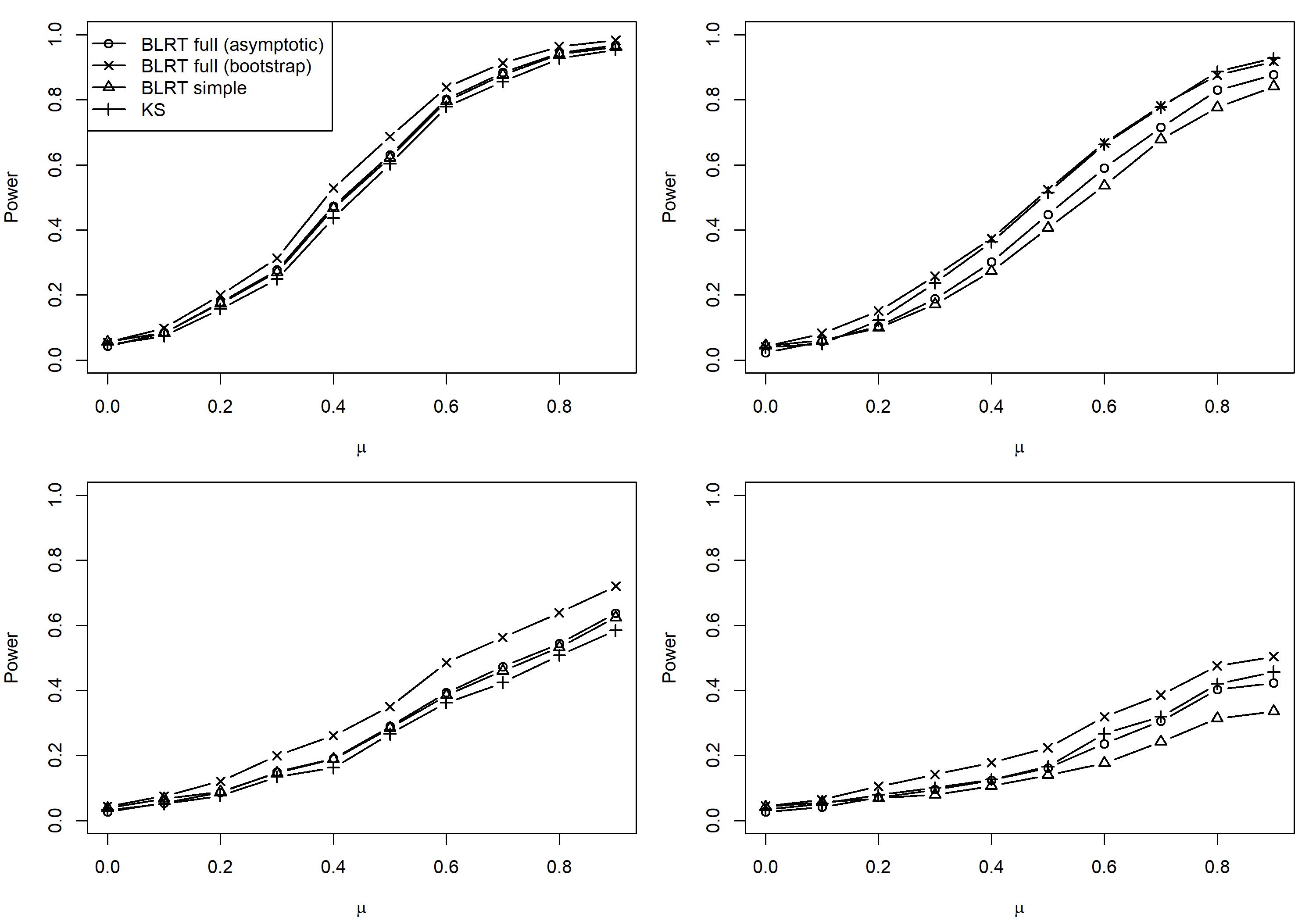
Table 1 shows estimated size and power of , , and from 1000 simulated datasets. This table reports the four simulation settings for and . Other values of are not reported in this table, but are plotted in Figure 1. More simulation results are reported in the Supplementary Materials (Section G). The first row of each simulation setting shows the simulated size. For power comparisons, one of the main findings is that the shape difference between and is important for the performances of the tests. When , and differ at tails, and and outperforms . However, when , and differ mostly at the middle, and outperforms the others. For another finding, when an IV is weak, meaning that is small, power is reduced, but at the same time, the shape difference between and is less centered since and dominate the shape. Therefore, as decreases, can capture the distributional difference more and produce better performance than . This can be found in Figure 1 by comparing the upper right plot and lower right plot; the asymptotic is less powerful than when an IV is strong, but they have the almost same power in the weak IV setting. In summary, when the difference of the distributions in two samples is not concentrated in the middle, and can be powerful.
As we pointed out in the previous section, the simulation results indicate that using the limiting distribution for is conservative. The simulated sizes do not reach the nominal level 0.05. We conducted additional simulations for various values when there is no effect at all. We conducted simulations for different sample sizes and the estimated sizes from 10,000 simulations for each are when . As we expected, the size approaches to the correct nominal level as increases. However, the convergence for is not satisfactory for a moderately large . This conservativeness essentially lowers the performance of in finite samples.
To boost the finite-sample performance, we can consider the bootstrapping method that simulates the true null distribution of under the null hypothesis for given . Bootstrapping can be done using the estimates and that are obtained under the null hypothesis. For the th procedure of bootstrapping, first fix and sample the compliance class membership using . Second, determine based on and ; for instance, if and , then . Third, take a sample based on and using the estimate . Finally, repeat the entire process for to obtain the bootstrapped samples . Table 1 reports simulated size and power based on bootstrapped samples for each simulated dataset. The column of (boot.) in Table 1 shows the estimated size and power from the bootstrap procedure. All the values are improved from the asymptotic-version values. The bootstrap-version can reduce the performance gap in cases where is superior, and in some cases, can overtake .
5.3 Simulation: Performance of the MBL Method
In this section, we evaluate the MBL estimates by comparing it with the plug-in estimates (3) and the estimates obtained from the rearrangement method proposed by Chernozhukov et al., (2010).
We consider the four situations in simulation studies. In the first three situations, all distributions are Gamma distributions: and . The compliance class proportions are (1) , (2) , (3) . In the fourth situation, all distributions are normal distributions: and with . The sample size is . To compute the average performance, we consider 1000 simulated datasets. For each dataset, we compute the distance between the estimated function and the true function , .
| Situation | Method | Bias | SE | 1000MSE |
|---|---|---|---|---|
| 1 | Plug-in | 0.0514 | 0.0923 | 11.16 |
| MBL | 0.0288 | 0.0330 | 1.92 | |
| Rearrangement | 0.0359 | 0.0740 | 6.76 | |
| 2 | Plug-in | 0.0098 | 0.0101 | 0.20 |
| MBL | 0.0088 | 0.0089 | 0.16 | |
| Rearrangement | 0.0087 | 0.0094 | 0.16 | |
| 3 | Plug-in | 0.0032 | 0.0032 | 0.02 |
| MBL | 0.0031 | 0.0031 | 0.02 | |
| Rearrangement | 0.0030 | 0.0031 | 0.02 | |
| 4 | Plug-in | 0.0612 | 0.1745 | 34.20 |
| MBL | 0.0276 | 0.0328 | 1.84 | |
| Rearrangement | 0.0255 | 0.0404 | 2.28 |
Table 2 shows the average performance of three considered estimation methods. Biases, standard errors and mean squared errors are reported. The MBL method has the least bias in situation 1, but the rearrangement method has the least bias in situations 2, 3 and 4. However, the MBL method has the least standard errors in every situation. Moreover, it has the best mean squared error in all the situations, although it has similar performance to the rearrangement method when an instrument is not weak.
6 Oregon Health Insurance Experiment: The Effect of Medicaid Coverage on Mental Health
We consider the 2008 Oregon health insurance experiment data that is publicly available from https://www.nber.org/oregon/1.home.html. To investigate the effect of Medicaid on health outcomes, Oregon opened a waiting list for a limited number of spots in its Medicaid program for low-income, uninsured, able-bodied adults between 19-64, which had previously been closed to new enrollment. From the waiting list, people selected by random lottery drawings, won the opportunity for themselves, and any household member, to apply for Oregon Health Program (OHP) Standard. However, not all persons selected by the lottery enrolled in Medicaid, either because they did not apply or because they were deemed ineligible. The lottery process and OHP standard are described in more detail in Finkelstein et al., (2012). This random assignment embedded in the lottery allows us to study the effect of Medicaid coverage in a random encouragement design. An indicator of winning a lottery is the instrumental variable. Also, enrollment to the Medicaid program is the non-randomized treatment variable. Approximately 2 years after the lottery, health outcomes are measured for persons who responded to the follow-up survey. In our example, we use a self-reported mental health outcome by using scores on the Medical Outcome Study 8-Item Short-Form Survey (SF-8). The scores range from 0 to 100, with higher scores indicating better self-reported health-related quality of life. The scale is normalized to yield a mean of 50 and a standard deviation of 10 in the general U.S. population. Details of other health outcomes and data collection have been provided in Baicker et al., (2013).
From the data, we consider a sample of 1,117 African Americans (single-person households) who signed themselves up for the lottery. Among them, 546 people (48.9%) were selected by the lottery drawings. The probability of Medicaid coverage is 0.511 in the lottery winning group and 0.226 in the other group. The plug-in estimates of the proportions for compliance classes are . Lottery selection increased the probability of Medicaid coverage by 28.5 points among the single-person African American households. The MBL estimates of the proportions are the same as the plug-in estimates up to three decimal places. The two-stage least squares (2SLS) estimate is 4.88 (95% CI, 0.01 to 9.75) with -value 0.050. The magnitude of improvement was approximately half of the standard deviation of the mental-component score. Furthermore, we can restrict our attention to a subsample of African Americans aged between 19-34 (). The 2SLS estimate is 9.92 (95% CI, 0.98 to 18.86) with -value 0.030. The estimated proportions of compliance classes are which are almost identical to the estimated proportions for the total African American population.

Figure 2 shows the estimated distribution functions of the potential outcomes of mental-component scores for compliers when enrolled in the Medicaid program and when not enrolled. The left plot shows the plug-in estimates described in Section 2.2 and the MBL estimates for African Americans aged between 19-64 (the full sample), and the right plot shows them for African Americans aged between 19-34. In both of the plots, we see that the estimated distribution function for complier without Medicaid coverage is almost always above the other. The gap between the two functions is wider at higher mental-component scores. Unlike the plug-in estimate, the MBL estimate satisfies the non-decreasing condition, and, as a result, there is a unique value of estimated scores corresponding to a specific quantile level. This feature can be useful for those who want to estimate the treatment effect at a certain quantile level using the estimated distribution functions. For example, the MBL method estimates that Medicaid coverage led to an increase of 8.70 points in the median score on the mental component for compliers. However, from the plug-in method, there are two values that correspond to the value 0.5 of the distribution for complier with Medicaid coverage, making it unclear how to compare the medians of the two distribution functions. For the young African American population (aged between 19-34), Medicaid coverage increased the median mental-component score by 14.68 points from 38.13 to 52.81.
Furthermore, the BLRT can be conducted for testing the null hypothesis . We apply both versions of the proposed binomial likelihood test, and , and compare them with . Using the asymptotic null distribution , the -values are computed as for . Moreover, the -value of can be computed by the bootstrap procedure with described in Section 5.2, and the -value is 0.021, which agrees with the asymptotic version of the -value. Similarly, for the young African American population, the estimated -values are for . For a smaller sample size, the proposed BLRT produced a smaller -value. For all considered tests, we reject the null hypothesis of equality of distributions at a significance level .
Finally, using the BLRT, we also test another hypothesis for testing treatment effect heterogeneity. All possible values of are examined for the African American population and the subpopulation of African Americans aged between 19-34. For the African American population, is not rejected for values between . Also, for African Americans aged between 19-34, is not rejected for values between . These results show that there is no evidence of treatment effect heterogeneity.
7 Discussion
We propose a non-parametric composite likelihood approach, referred to as the binomial likelihood (BL) method, for making causal inferences about the distributional treatment effect in a randomized experiment with an instrumental variable. The BL approach provides a non-parametric inferential tool similar to the classical parametric likelihood. The maximum binomial likelihood (MBL) method provides estimates of the outcome distributions, which are proper distribution functions and the binomial likelihood ratio test (BLRT) is a powerful technique to detect distributional changes when the outcome distributions are close to each other, especially when the IV is weak.
Several extensions and generalizations of the BL method are possible. For instance, while constructing the BL functions one requires specification of the knots as evaluating points. We recommended to use all the observed outcomes for the knots, but a different specification can be considered depending on the question of interest. For example, in the Oregon Health Insurance experiment, if one wants to examine whether there is any effect for people above mental score 40, then only outcomes above 40 can be chosen as knots. In such a setting, a rejection implies that there is evidence of distributional changes for this specific subpopulation.
The results in this paper show that the BL approach works well in randomized encouragement experiments where a compliance class is latent. A possible future direction could be to study the performance of the BL approach in general mixture models when there is a latent variable.
Acknowledgement
The authors thank Abhishek Chakrabortty and Shirshendu Ganguly for helpful discussions.
References
- Abadie, (2002) Abadie, A. (2002). Bootstrap tests for distributional treatment effects in instrumental variable models. Journal of the American Statistical Association, 97(457):284–292.
- Abadie, (2003) Abadie, A. (2003). Semiparametric instrumental variable estimation of treatment response models. Journal of Econometrics, 113(2):231–263.
- Angrist et al., (1996) Angrist, J. D., Imbens, G. W., and Rubin, D. B. (1996). Idenrification of causal effects using instrumental variables. Journal of the American Statistical Association, 91(434):444–455.
- Baicker et al., (2013) Baicker, K., Taubman, S. L., Allen, H. L., Bernstein, M., Gruber, J. H., Newhouse, J. P., Schneider, E. C., Wright, B. J., Zaslavsky, A. M., and Finkelstein, A. N. (2013). The Oregon experiment – effects of Medicaid on clinical outcomes. New England Journal of Medicine, 368(18):1713–1722.
- Baiocchi et al., (2014) Baiocchi, M., Cheng, J., and Small, D. S. (2014). Instrumental variable methods for causal inference. Statistics in Medicine, 33(13):2297–2340.
- Brookhart and Schneeweiss, (2007) Brookhart, M. A. and Schneeweiss, S. (2007). Preference-based instrumental variable methods for the estimation of treatment effects: assessing validity and interpreting results. The International Journal of Biostatistics, 3(1).
- (7) Cheng, J., Qin, J., and Zhang, B. (2009a). Semiparametric estimation and inference for distributional and general treatment effects. Journal of the Royal Statistical Society: Series B (Statistical Methodology), 71(4):881–904.
- (8) Cheng, J., Small, D. S., Tan, Z., and Ten Have, T. R. (2009b). Efficient nonparametric estimation of causal effects in randomized trials with noncompliance. Biometrika, 96(1):19–36.
- Chernozhukov et al., (2010) Chernozhukov, V., Fernandez-Val, I., and Galichon, A. (2010). Quantile and probability curves without crossing. Econometrica, 78(3):1093–1125.
- Finkelstein et al., (2012) Finkelstein, A., Taubman, S., Wright, B., Bernstein, M., Gruber, J., Newhouse, J. P., Allen, H., Baicker, K., and Oregon Health Study Group (2012). The Oregon health insurance experiment: evidence from the first year. The Quarterly journal of economics, 127(3):1057–1106.
- Geman and Hwang, (1982) Geman, S. and Hwang, C.-R. (1982). Nonparametric maximum likelihood estimation by the method of sieves. The Annals of Statistics, 10(2):401–414.
- Heagerty and Lele, (1998) Heagerty, P. J. and Lele, S. R. (1998). A composite likelihood approach to binary spatial data. Journal of the American Statistical Association, 93(443):1099–1111.
- Hernan and Robins, (2006) Hernan, M. A. and Robins, J. M. (2006). Instruments for causal inference: an epidemiologist’s dream? Epidemiology, 17(4):360–372.
- Holland, (1988) Holland, P. W. (1988). Causal inference, path analysis, and recursive structural equations models. Sociological Methodology, 18:449–484.
- Johnson et al., (2019) Johnson, M., Cao, J., and Kang, H. (2019). Detecting heterogeneous treatment effect with instrumental variables. arXiv preprint arXiv:1908.03652.
- Kang et al., (2018) Kang, H., Peck, L., and Keele, L. (2018). Inference for instrumental variables: a randomization inference approach. Journal of the Royal Statistical Society: Series A (Statistics in Society), 181(4):1231–1254.
- Larribe and Fearnhead, (2011) Larribe, F. and Fearnhead, P. (2011). On composite likelihoods in statistical genetics. Statistica Sinica, 21(1):43–69.
- Lindsay, (1988) Lindsay, B. G. (1988). Composite likelihood methods. Contemporary Mathematics, 80(1):221–39.
- Neyman, (1923) Neyman, J. (1923). On the application of probability theory to agricultural experiments. Roczniki Nauk Roiniczych, X:1–51. Reprinted in Statistical Science, 1990, 5, 463–485.
- Ogburn et al., (2015) Ogburn, E. L., Rotnitzky, A., and Robins, J. M. (2015). Doubly robust estimation of the local average treatment effect curve. Journal of the Royal Statistical Society: Series B (Statistical Methodology), 77(2):373–396.
- Owen, (2001) Owen, A. B. (2001). Empirical likelihood. Chapman & Hall/CRC Press.
- Pettitt, (1976) Pettitt, A. N. (1976). A two-sample Anderson-Darling rank statistic. Biometrika, 63(1):161–168.
- Rubin, (1974) Rubin, D. B. (1974). Estimating causal effects of treatments in randomized and nonrandomized studies. Journal of educational Psychology, 66(5):688–701.
- Rubin, (1986) Rubin, D. B. (1986). Statistics and causal inference: Comment: which ifs have causal answers. Journal of the American Statistical Association, 81(396):961–962.
- Rubin, (1998) Rubin, D. B. (1998). More powerful randomization-based p-values in double-blind trials with non-compliance. Statistics in Medicine, 17(3):371–385.
- Scholz and Stephens, (1987) Scholz, F. W. and Stephens, M. A. (1987). K-sample Anderson–Darling tests. Journal of the American Statistical Association, 82(399):918–924.
- Tan, (2006) Tan, Z. (2006). Regression and weighting methods for causal inference using instrumental variables. Journal of the American Statistical Association, 101(476):1607–1618.
- Varin et al., (2011) Varin, C., Reid, N., and Firth, D. (2011). An overview of composite likelihood methods. Statistica Sinica, 21(1):5–42.