Ab initio electronic structure of quasi two-dimensional materials: a “native” gaussian–plane wave approach

Following the successful isolation of single-layer graphene in 2004 Novoselov, the study of quasi two-dimensional materials – either single atomic layers or stacks of a few layers – has become one of the most important areas of research in materials science. It is expected that the unprecedented flexibility of these materials, which can be assembled in many different combinations, including insulating, metallic, and superconducting layers, will lead in time to major technological advances. Basic physics concepts such as massless Dirac Fermions and coupled valley-spin dynamics can also be studied in these systems. From the point of view of computational electronic structure theory the challenge is to reliably predict the properties of a quasi-2D structure with minimal input from experiment. Ideally we would like to be able to decide, based on computation, which structures are stable, which are metals and which are insulators, what their excitation spectra look like. Most of the methods that are presently in use in solid state physics to address these questions – Kohn-Sham density functional theory, GW approximations, Bethe-Salpeter (BS) equations, dynamical mean field theory – have been developed for 3D systems and are now being applied to quasi-2D systems (important exceptions are OctopusOctopus and GPAW gpaw, which allow the user to specify a reduced number of periodic directions).

However, the transition from 3D to quasi-2D is not free of pitfalls. Bulk 3D crystals exhibit periodicity in all three directions and are treated with the help of periodic boundary conditions. This means, in practice, that computational methods are implemented on a basis of wave functions that exhibit three-dimensional periodicity, such as plane waves Gonze20092582; QE-2009; gpaw; PhysRevB.54.11169, augmented plane waves (APW) Exciting!; elk-code; PhysRevB.81.125102, LMTO LMsuite or periodic sums of atomic orbitals Fhi-Aims; Siesta; gpaw; Octopus. Quasi 2D materials on the other hand, have crystalline periodicity in two dimensions only. In the third direction (which we will call the $z$-direction) the wave function is that of a polyatomic molecule, possibly a very large one, but in any case decaying exponentially at sufficiently large distance from the atomic layers. Therefore, strictly speaking, periodic boundary conditions cannot be used in the third direction. Another key difference is that, due to the quasi-two dimensional character of the electronic charge distribution, electric field fluctuations are not screened at sufficiently large distance in the plane of the layers PhysRevB.84.085406; PhysRevB.92.245123: therefore electron-electron interaction effects are much stronger than in conventional 3D materials.

It turns out that these difficulties are connected. In order to keep using 3D computer codes with periodic basis sets it is customary to resort to an artifice known as the “supercell method”, whereby the quasi-2D material is periodically repeated in the $z$ direction. The distance between the artificial replicas, $d$, is chosen to be large in the hope that interaction effects between the replicas can be ignored. If everything goes well, the results should become independent of $d$ in the limit $d\to\infty$. Unfortunately, because of the failure of screening, the Coulomb interaction between artificial replicas decreases very slowly with increasing $d$, and may cause spurious results. In addition the exchange-correlation potentials of density functional theory, when treated exactly, are known to be highly nonlocal functionals of the density, which decay very slowly, with the inverse of the distance from the plane of the material Lang_Kohn; vBarth; Silkin. The problem is particularly acute in the calculation of dynamical response properties, where the replicas create an artificial dynamical environment.

To counter these difficulties two main techniques have been developed so far. The first  Rozzi_cutoff; Castro_cutoff relies on truncating the Coulomb interaction beyond a certain cutoff distance in the $z$ direction. Thus one hopes eliminate the unphysical interaction between the replicas while preserving the long-range interaction within the physical layer, or set of layers. Another solution Nazarov_2d is to calculate the mean field created by the replicas and subtract it from the field that acts on the electrons in the physical layer: for the dynamical dielectric function and related properties this can be done in a relatively inexpensive way.

Ultimately, the best and most elegant solution would be to do the calculations with a code that recognizes at the outset the quasi-2D character of the system and takes advantage of its structure by using a basis set of wave functions that are periodic (plane-wave like) in the $(x,y)$ plane and atomic-like in the $z$-direction. We refer to such a code as a “native” quasi-2D code. A similar approach has been proposed, very recently, in Ref. [PhysRevB.92.115132], where the full-potential linearized augmented plane-wave method is modified to account for the exponential decay of the basis function in the $z$-direction.

In this paper we take a first step towards the construction of a native quasi-2D code by introducing a set of basis functions with the properties outlined above, and by showing how some of the basic tools of ab initio electronic structure theory – density functional theory, GW approximation and Bethe-Salpeter equation – are implemented in this basis. Our approach is inspired by the FHI-AIMS basis set, in which periodic functions in 3D are constructed from Bloch sums of numerically generated Natural Atom-centred Orbitals (NAO) - see Appendix C. We insert these orbitals into two-dimensional Bloch sums to arrive at the desired basis functions. While the FHI-AIMS code is already able to perform “native” Kohn-Sham DFT on a quasi-2D basis, our implementation of GW and BS equations on this basis set is new and will prove to be a powerful and versatile tool for the calculation of electronic properties of quasi-2D materials.

It might be objected that the use of NAO orbitals for the $z$-dependence of the wave function will become unpractical (i.e., require many terms for good convergence) when the wave function is very extended in that direction, as is the case for high-energy unoccupied states. This is partially true, but we counter that (i) these extended states would become anyway unreliable when treated in the conventional supercell method, due to spurious cross-talk between replicas, (ii) extended basis sets have recently been developed and optimized to treat the excited states in FHI-AIMSExtended_aims1; Extended_aims2, and (iii) a new technology exists, based on the Sternheimer equation PhysRevB.81.115105; PhysRevB.88.075117 to avoid the use of excited states in the implementation of the GW method. Finally, we expect that the two-dimensional implementation of these tasks will speed up the calculations and make them more reliable, once the required computer codes are fully developed.

This paper is organized as follows: in section II we introduce the quasi-2D basis functions and review their formal properties. In particular, because these functions are not mutually orthogonal, we find it convenient to introduce covariant and contravariant components of vectors in the Hilbert space – the two types of components being connected by a “metric tensor”, which is the matrix of the overlaps. In section III, the two space point functions are described in this new formalism. Therefore, we represent the Dyson equation for the GW self-energy (section IV), the polarization function (section V) and screened potential W (section VI) on the quasi-2D basis. Finally, in section VII, the BS equation for the two-particle propagator on the quasi-2D basis is made explicit and we introduce the effective two-band exciton equation (sub section VII.1). The last section VIII contains our summary and outlook for the development of the ideas presented in this paper. In appendix A a single pole approximation is revisited. In appendix B, the contour integration technique for the GWA is derived in our formalism. Finally, a brief overview of the FHI-AIMS NAO orbitals is provided in appendix C.

For a system that is periodic in the $(x,y)$ plane, but not in the $z$ direction – an array of molecules arranged in a 2D lattice – we introduce basis functions of the Bloch type, characterized by a Bloch wave vector ${\bf k}$ in the $(x,y)$ plane. The general form of these basis functions is PhysRevB.48.17791; PhysRevLett.75.3489; PhysRevB.62.4927

$$\chi_{\alpha{\bf k}}(\mbox{\boldmath$\xi$})\equiv\frac{1}{\sqrt{N}}\sum_{{\bf R}}e^{i{\bf k}\cdot{\bf R}}\phi_{nlm}(\mbox{\boldmath$\xi$}-{\bf R}-{\bf d}_{a})$$

(1)

where $\mbox{\boldmath$\xi$}=({\bf x},z)$ is a three dimensional position vector; ${\bf R}$ is a lattice vector in the $(x,y)$ plane, ${\bf d}_{a}$ is a three-dimensional vector specifying the position of the $a$-th atom in the two-dimensional unit cell labelled by ${\bf R}$, and $\phi_{nlm}(\mbox{\boldmath$\xi$}-{\bf R}-{\bf d}_{a})$ are orthonormal atomic orbitals labeled by atomic quantum numbers $(n,l,m)$ and centered at ${\bf R}+{\bf d}_{a}$. $N$ is the number of cells in the two-dimensional lattice, and $\alpha=n,l,m,a$ is a composite index including the atomic quantum numbers and the position of the atom in the unit cell. The form of the $\phi$ orbitals will be left unspecified for the time being: explicit numerical expressions that are used in the FHI-AIMS code will be discussed later (see Appendix B). Note that

$$\chi_{\alpha{\bf k}}(\mbox{\boldmath$\xi$}+{\bf R})=e^{i{\bf k}\cdot{\bf R}}\chi_{\alpha{\bf k}}(\mbox{\boldmath$\xi$})\,,$$

(2)

as required for a Bloch wave of wave vector ${\bf k}$.

The basis functions satisfy the “orthonormality” relation

$$\int d\mbox{\boldmath$\xi$}\chi^{*}_{\alpha{\bf k}}(\mbox{\boldmath$\xi$})\chi_{\beta{\bf p}}(\mbox{\boldmath$\xi$})\equiv S_{\alpha\beta}({\bf k})\delta_{{\bf k},{\bf p}}\,,$$

(3)

where $S_{\alpha\beta}({\bf k})=S^{*}_{\beta\alpha}({\bf k})$ is a hermitian matrix. In addition to the covariant basis functions of Eq. (1) it is convenient to introduce the contravariant basis set

$$\chi^{\alpha}_{{\bf k}}(\mbox{\boldmath$\xi$})\equiv\sum_{\beta}S^{\alpha\beta}({\bf k})\chi_{\beta{\bf k}}(\mbox{\boldmath$\xi$})$$

(4)

where $S^{\alpha\beta}({\bf k})\equiv[S^{-1}({\bf k})]_{\beta\alpha}$ is the transposed inverse of the “metric tensor” $S({\bf k})$. In Quantum Chemistry, $S^{\alpha\beta}$ is referred as overlap matrix. In terms of covariant and contravariant basis elements the “orthonormality” relations take the simpler form

$$\int d\mbox{\boldmath$\xi$}\chi^{\alpha*}_{{\bf k}}(\mbox{\boldmath$\xi$})\chi_{\beta{\bf p}}(\mbox{\boldmath$\xi$})=\delta_{\alpha\beta}({\bf k})\delta_{{\bf k},{\bf p}}\,.$$

(5)

We can also write the completeness relation in the form

$$\sum_{\alpha{\bf k}}\chi_{\alpha{\bf k}}(\mbox{\boldmath$\xi$})\chi^{\alpha*}_{{\bf k}}(\mbox{\boldmath$\xi$}^{\prime})=\delta(\mbox{\boldmath$\xi$}-\mbox{\boldmath$\xi$}^{\prime})\,,$$

(6)

where the sum over ${\bf k}$ runs over the vectors of the first Brillouin zone of the reciprocal 2D lattice. This is evident from the fact that for an arbitrary function $f(\bm{\xi})=\sum_{\beta{\bf p}}f^{\beta}_{{\bf p}}\chi_{\beta{\bf p}}(\bm{\xi})$ we have, by virtue of Eq. (5),

$$\int d\bm{\xi}^{\prime}\sum_{\alpha{\bf k}}\chi_{\alpha{\bf k}}(\mbox{\boldmath$\xi$})\chi^{\alpha*}_{{\bf k}}(\mbox{\boldmath$\xi$}^{\prime})f(\bm{\xi}^{\prime})=\sum_{\alpha{\bf k}}f^{\alpha}_{{\bf k}}\chi_{\alpha{\bf k}}(\bm{\xi})=f(\bm{\xi})\,.$$

(7)

A Bloch wave function $\psi_{{\bf k}}(\mbox{\boldmath$\xi$})$ in the Hilbert space can be expressed as a contravariant vector as follows:

$$\psi_{\bf k}(\mbox{\boldmath$\xi$})=\sum_{\alpha}\psi_{{\bf k}}^{\alpha}\chi_{\alpha{\bf k}}(\mbox{\boldmath$\xi$})\,,~~~{\rm where}~~~\psi_{{\bf k}}^{\alpha}=\int d\mbox{\boldmath$\xi$}\chi^{\alpha*}_{{\bf k}}(\mbox{\boldmath$\xi$})\psi_{{\bf k}}(\mbox{\boldmath$\xi$})\,.$$

(8)

The scalar product of two Bloch wave functions $\psi_{{\bf k}}(\mbox{\boldmath$\xi$})$ and $\varphi_{{\bf k}}(\mbox{\boldmath$\xi$})$ is then given by

$$(\psi_{{\bf k}},\varphi_{{\bf k}})=\int d\mbox{\boldmath$\xi$}\psi^{*}_{{\bf k}}(\mbox{\boldmath$\xi$})\varphi_{{\bf k}}(\mbox{\boldmath$\xi$})=\sum_{\alpha}\psi^{*}_{{\bf k}\alpha}\varphi_{{\bf k}}^{\alpha}=\sum_{\alpha}\psi^{*\alpha}_{{\bf k}}\varphi_{{\bf k}\alpha}\,.$$

(9)

Covariant and contravariant components of the same vector are connected by the metric tensor:

$$\psi_{{\bf k}\alpha}=\sum_{\beta}\psi_{{\bf k}}^{\beta}S_{\beta\alpha}({\bf k})\,.$$

(10)

In the following, the solutions of, say, the Kohn-Sham equations for a given layered structure will be represented as covariant or contravariant vectors in the hybrid atomic-plane wave basis.

We now consider the representation of a periodic two-point function $f(\mbox{\boldmath$\xi$},\mbox{\boldmath$\xi$}^{\prime})$, i.e., a function such that

$$f(\mbox{\boldmath$\xi$}+{\bf R},\mbox{\boldmath$\xi$}^{\prime}+{\bf R})=f(\mbox{\boldmath$\xi$},\mbox{\boldmath$\xi$}^{\prime})\,,$$

(11)

where ${\bf R}$ is a two-dimensional lattice vector. Making use of the completeness relation (6) we easily see that

$$f(\mbox{\boldmath$\xi$},\mbox{\boldmath$\xi$}^{\prime})=\sum_{\alpha\beta{\bf k}}\chi_{\alpha{\bf k}}(\mbox{\boldmath$\xi$})f^{\alpha\beta}({\bf k})\chi_{\beta{\bf k}}^{*}(\mbox{\boldmath$\xi$}^{\prime})\,,~~~~{\rm where}~~~f^{\alpha\beta}({\bf k})=\int d\mbox{\boldmath$\xi$}d\mbox{\boldmath$\xi$}^{\prime}\chi^{*\alpha}_{{\bf k}}(\mbox{\boldmath$\xi$})f(\mbox{\boldmath$\xi$},\mbox{\boldmath$\xi$}^{\prime})\chi^{\beta}_{{\bf k}}(\mbox{\boldmath$\xi$}^{\prime})$$

(12)

or, alternatively

$$f(\mbox{\boldmath$\xi$},\mbox{\boldmath$\xi$}^{\prime})=\sum_{\alpha\beta{\bf k}}\chi^{\alpha}_{{\bf k}}(\mbox{\boldmath$\xi$})f_{\alpha\beta}({\bf k})\chi^{*\beta}_{{\bf k}}(\mbox{\boldmath$\xi$}^{\prime})\,,~~~~{\rm where}~~~f_{\alpha\beta}({\bf k})=\int d\mbox{\boldmath$\xi$}d\mbox{\boldmath$\xi$}^{\prime}\chi^{*}_{\alpha{\bf k}}(\mbox{\boldmath$\xi$})f(\mbox{\boldmath$\xi$},\mbox{\boldmath$\xi$}^{\prime})\chi_{\beta{\bf k}}(\mbox{\boldmath$\xi$}^{\prime})$$

(13)

We notice in passing that the first of Eqs. (12) and the second of Eqs. (13) correspond, respectively, to Eqs. (6) and (7) of Ref. PhysRevB.48.17791, i.e., $f^{\alpha\beta}$ and $f_{\alpha\beta}$ correspond, respectively, to the “angular bracket” and “square bracket” matrix elements of Ref. PhysRevB.48.17791.

These representations apply, in particular to the Green’s function $G(\mbox{\boldmath$\xi$},\mbox{\boldmath$\xi$}^{\prime},\omega)$ and the screened electron-electron interaction $W(\mbox{\boldmath$\xi$},\mbox{\boldmath$\xi$}^{\prime},\omega)$. We now show how the two representations are combined in the GW approximation.

As an example, consider the noninteracting Green’s function (advanced and retarded Green’s function):

$$G_{0}(\mbox{\boldmath$\xi$},\mbox{\boldmath$\xi$}^{\prime},\omega)=\sum_{n{\bf k}}\frac{\psi_{n{\bf k}}(\mbox{\boldmath$\xi$})\psi_{n{\bf k}}^{*}(\mbox{\boldmath$\xi$}^{\prime})}{\omega-E_{n{\bf k}}\pm i0^{+}}\,.$$

(14)

Then, expanding in Bloch functions:

$$G_{0}^{\alpha\beta}({\bf k},\omega)=\sum_{n}\frac{\psi^{\alpha}_{n{{\bf k}}}\psi^{\beta*}_{n{\bf k}}}{\omega-E_{n{\bf k}}\pm i0^{+}}$$

(15)

where $\psi_{n{\bf k}}(\bm{\xi})\equiv\sum_{\alpha}\psi^{\alpha}_{n{{\bf k}}}\chi_{\alpha{\bf k}}(\mbox{\boldmath$\xi$})$ are non-interacting one- electron wave functions and $E_{n{\bf k}}$ the one-electron energies.

In the GW approximation the self-energy is a parallel convolution product of G and W, usually approximated by their lowest-order forms $G_{0}$ and $W_{0}$:

$$\Sigma(\mbox{\boldmath$\xi$},\mbox{\boldmath$\xi$}^{\prime},\omega)=\frac{i}{2\pi}G_{0}(\mbox{\boldmath$\xi$},\mbox{\boldmath$\xi$}^{\prime},\omega)*W_{0}(\mbox{\boldmath$\xi$},\mbox{\boldmath$\xi$}^{\prime},\omega)e^{-i\eta\omega}\,.$$

(16)

Here the $*$ represent the convolution product: $f(\omega)*g(\omega)\equiv\int d\omega^{\prime}f(\omega-\omega^{\prime})g(\omega^{\prime})$ and . The corresponding diagram is shown in Fig. (1).

We expand the product as

$$\Sigma(\mbox{\boldmath$\xi$},\mbox{\boldmath$\xi$}^{\prime},\omega)=\sum_{{\bf p}^{\prime}{\bf q}}G_{0}^{\alpha\beta}({\bf p}^{\prime},\omega)\chi_{\alpha{\bf p}^{\prime}}(\mbox{\boldmath$\xi$})\chi^{*}_{\beta{\bf p}^{\prime}}(\mbox{\boldmath$\xi$}^{\prime})*W_{0,\gamma\delta}({\bf q},\omega)\chi^{\gamma}_{{\bf q}}(\mbox{\boldmath$\xi$})\chi^{*\delta}_{{\bf q}}(\mbox{\boldmath$\xi$}^{\prime})$$

(17)

where the sum over repeated indices is understood. Then the matrix element of the self-energy is

$$\Sigma_{\mu\nu}({\bf p},\omega)=\frac{i}{2\pi}\sum_{{\bf p}^{\prime}{\bf q}}\left[\int d\mbox{\boldmath$\xi$}\chi^{*}_{\mu{\bf p}}(\mbox{\boldmath$\xi$})\chi_{\alpha{\bf p}^{\prime}}(\mbox{\boldmath$\xi$})\chi^{\gamma}_{{\bf q}}(\mbox{\boldmath$\xi$})\right]G_{0}^{\alpha\beta}({\bf p}^{\prime},\omega)\left[\int d\mbox{\boldmath$\xi$}^{\prime}\chi^{*}_{\beta{\bf p}^{\prime}}(\mbox{\boldmath$\xi$}^{\prime})\chi^{*\delta}_{{\bf q}}(\mbox{\boldmath$\xi$}^{\prime})\chi_{\nu{\bf p}}(\mbox{\boldmath$\xi$}^{\prime})\right]*W_{0,\gamma\delta}({\bf q},\omega)$$

(18)

The quantities in the square brackets vanish unless ${\bf p}^{\prime}={\bf p}-{\bf q}$. We define

$$\int d\mbox{\boldmath$\xi$}\chi^{*}_{\mu{\bf p}}(\mbox{\boldmath$\xi$})\chi_{\alpha{\bf p}^{\prime}}(\mbox{\boldmath$\xi$})\chi^{\gamma}_{{\bf q}}(\mbox{\boldmath$\xi$})\equiv\Gamma^{\gamma}_{\mu\alpha}({\bf p},{\bf p}-{\bf q})$$

(19)

and

$$\int d\mbox{\boldmath$\xi$}^{\prime}\chi^{*}_{\beta{\bf p}^{\prime}}(\mbox{\boldmath$\xi$}^{\prime})\chi^{*\delta}_{{\bf q}}(\mbox{\boldmath$\xi$}^{\prime})\chi_{\nu{\bf p}}(\mbox{\boldmath$\xi$}^{\prime})\equiv\Gamma^{\delta}_{\beta\nu}({\bf p}-{\bf q},{\bf p})\,.$$

(20)

These matrix elements are illustrated in Fig. (1 (b)). Note that $\Gamma^{\delta}_{\beta\nu}({\bf p}-{\bf q},{\bf p})=[\Gamma^{\delta}_{\nu\beta}({\bf p},{\bf p}-{\bf q})]^{*}$. Then complete result for the self-energy is

$$\Sigma_{\mu\nu}({\bf p},\omega)=\frac{i}{2\pi}\sum_{{\bf q}}\Gamma^{\gamma}_{\mu\alpha}({\bf p},{\bf p}-{\bf q})G_{0}^{\alpha\beta}({\bf p}-{\bf q},\omega)\Gamma^{\delta}_{\beta\nu}({\bf p}-{\bf q},{\bf p})*W_{0,\gamma\delta}({\bf q},\omega)$$

(21)

Another crucial two-point function is the polarization function. The noninteracting polarization function is an antiparallel convolution of two Green’s functions

$$P_{0}(\mbox{\boldmath$\xi$},\mbox{\boldmath$\xi$}^{\prime},\omega)=G_{0}(\mbox{\boldmath$\xi$},\mbox{\boldmath$\xi$}^{\prime},\omega)*G_{0}(\mbox{\boldmath$\xi$}^{\prime},\mbox{\boldmath$\xi$},-\omega)\,,$$

(22)

where $*$ represents the convolution product. A graphical representation of this formula is shown in Fig. 2.

We expand the product as

$$P_{0}(\mbox{\boldmath$\xi$},\mbox{\boldmath$\xi$}^{\prime},\omega)=\sum_{{\bf p}{\bf p}^{\prime}}G_{0}^{\alpha\beta}({\bf p},\omega)\chi_{\alpha{\bf p}}(\mbox{\boldmath$\xi$})\chi^{*}_{\beta{\bf p}}(\mbox{\boldmath$\xi$}^{\prime})*G_{0}^{\gamma\delta}({\bf p}^{\prime},-\omega)\chi_{\gamma{\bf p}^{\prime}}(\mbox{\boldmath$\xi$}^{\prime})\chi^{*}_{\delta{\bf p}^{\prime}}(\mbox{\boldmath$\xi$})$$

(23)

Then the matrix element of the polarization propagator is

$$P_{0}^{\mu\nu}({\bf q},\omega)=\sum_{{\bf p}{\bf p}^{\prime}}\left[\int d\mbox{\boldmath$\xi$}\chi^{*\mu}_{\bf q}(\mbox{\boldmath$\xi$})\chi_{\alpha{\bf p}}(\mbox{\boldmath$\xi$})\chi^{*}_{\delta{\bf p}^{\prime}}(\mbox{\boldmath$\xi$})\right]G_{0}^{\alpha\beta}({\bf p},\omega)\left[\int d\mbox{\boldmath$\xi$}^{\prime}\chi^{*}_{\beta{\bf p}}(\mbox{\boldmath$\xi$}^{\prime})\chi^{\nu}_{{\bf q}}(\mbox{\boldmath$\xi$}^{\prime})\chi_{\gamma{\bf p}^{\prime}}(\mbox{\boldmath$\xi$}^{\prime})\right]*G_{0}^{\gamma\delta}({\bf p}^{\prime},-\omega)$$

(24)

Again, the quantities in the square brackets vanish unless ${\bf p}^{\prime}={\bf p}-{\bf q}$. With the three-point vertices $\Gamma$ defined in Eqs. (19) and  (20) we easily get the following representation of the polarization propagator:

$$P_{0}^{\mu\nu}({\bf q},\omega)=\sum_{{\bf p}}\Gamma^{\mu}_{\delta\alpha}({\bf p}-{\bf q},{\bf p})G_{0}^{\alpha\beta}({\bf p},\omega)\Gamma^{\nu}_{\beta\gamma}({\bf p},{\bf p}-{\bf q})*G_{0}^{\gamma\delta}({\bf p}-{\bf q},-\omega)$$

(25)

The covariant components of the RPA screened interaction can be obtained from the formula

$$W_{0,\alpha\beta}({\bf q},\omega)=[v^{1/2}({\bf q})]_{\alpha\gamma}[\tilde{\epsilon}^{-1}({\bf q},\omega)]^{\gamma\delta}[v^{1/2}({\bf q})]_{\delta\beta}\,.$$

(26)

Here

$$[v^{1/2}({\bf q})]_{\alpha\gamma}=\int d\mbox{\boldmath$\xi$}d\mbox{\boldmath$\xi$}^{\prime}\chi^{*}_{\alpha{\bf q}}(\mbox{\boldmath$\xi$})v^{1/2}(\mbox{\boldmath$\xi$},\mbox{\boldmath$\xi$}^{\prime})\chi_{\gamma{\bf q}}(\mbox{\boldmath$\xi$}^{\prime})$$

(27)

where

$$v^{1/2}(\mbox{\boldmath$\xi$},\mbox{\boldmath$\xi$}^{\prime})=\frac{e}{\pi^{3/2}|\mbox{\boldmath$\xi$}-\mbox{\boldmath$\xi$}^{\prime}|^{2}}\,,$$

(28)

is the “‘square root” of the Coulomb interaction. Further we have

$$\tilde{\epsilon}_{\alpha\beta}({\bf q},\omega)=S_{\alpha\beta}({\bf q})-[v^{1/2}({\bf q})]_{\alpha\gamma}P_{0}^{\gamma\delta}({\bf q},\omega)[v^{1/2}({\bf q})]_{\delta\beta}$$

(29)

A simple single-pole approximation for $\tilde{\epsilon}({\bf q},\omega)$ is described in the Appendix.

Besides one-particle properties, which are usually described in terms of the Kohn-Sham wave functions and the self-energy, two-particle properties also play a prominent role in computational materials science. For example, the information about the optical spectrum and the refractive index of materials is contained in the macroscopic dielectric function $\epsilon_{M}(\omega)$, which, in ordinary three-dimensional periodic systems, is defined as the ratio between the macroscopic external electric field and the macroscopic total electric field, where “macroscopic” means averaged over a region much larger than the size of the unit cell. For 2D materials care must be exerted to construct the appropriate response function for the experimental situation under studyNazarov_2d. In the case of optical properties, the macroscopic dielectric function reduces to $1$ and we focus instead on the longitudinal in-plane polarizability per unit cell, which we define as

$$\chi_{P}(\omega)=\frac{1}{N_{c}}\lim_{{\bf q}\to 0}\frac{e^{2}}{q^{2}}\int d\bm{\xi}\int d\bm{\xi}^{\prime}e^{-i{\bf q}\cdot({\bf r}-{\bf r}^{\prime})}\bar{L}(\bm{\xi},\bm{\xi},\bm{\xi}^{\prime},\bm{\xi}^{\prime};\omega)\,,$$

(30)

where $\bar{L}(\bm{\xi}_{1},\bm{\xi}_{2},\bm{\xi}_{3},\bm{\xi}_{4};\omega)$ is the proper four-point electron-hole propagator, integrated over the frequencies of the external legs and $N_{c}$ is the number of unit cells. We remind the reader that the most general form of the electron-hole propagator is $\bar{L}_{full}(\bm{\xi}_{1},\bm{\xi}_{2},\bm{\xi}_{3},\bm{\xi}_{4};\epsilon_{1},\epsilon_{2},\epsilon_{3},\epsilon_{4})$, where $\epsilon_{2}=\epsilon_{1}-\omega$ and $\epsilon_{4}=\epsilon_{3}-\omega$ are the frequencies of the external legs. The simpler propagator $L$ (still referred to as electron-hole propagator for brevity) is obtained from $L_{full}$ by integrating over $\epsilon_{1}$ and $\epsilon_{3}$ at fixed $\omega$. The bar over $L$ is a reminder that we are calculating $L$ with exclusion of the long-range Coulomb interaction rmp_onida in the so-called exchange electron-hole channel. To explain this point more clearly we recall that the interacting electron-hole propagator is given by the solution of the Bethe-Salpeter Equation (BSE) (Fig. 3 (a))

$$\begin{split}L(\mbox{\boldmath$\xi$}_{1},\mbox{\boldmath$\xi$}_{2},\mbox{\boldmath$\xi$}_{3},\mbox{\boldmath$\xi$}_{4};\omega)&=L_{0}(\mbox{\boldmath$\xi$}_{1},\mbox{\boldmath$\xi$}_{2},\mbox{\boldmath$\xi$}_{3},\mbox{\boldmath$\xi$}_{4};\omega)\\ &+\int d\mbox{\boldmath$\xi$}^{\prime}_{1}d\mbox{\boldmath$\xi$}^{\prime}_{2}d\mbox{\boldmath$\xi$}^{\prime}_{3}d\mbox{\boldmath$\xi$}^{\prime}_{4}L_{0}(\mbox{\boldmath$\xi$}_{1},\mbox{\boldmath$\xi$}_{2},\mbox{\boldmath$\xi$}_{1}^{\prime},\mbox{\boldmath$\xi$}_{2}^{\prime};\omega)I(\mbox{\boldmath$\xi$}^{\prime}_{1},\mbox{\boldmath$\xi$}_{2}^{\prime},\mbox{\boldmath$\xi$}_{3}^{\prime},\mbox{\boldmath$\xi$}_{4}^{\prime})L(\mbox{\boldmath$\xi$}_{3}^{\prime},\mbox{\boldmath$\xi$}_{4}^{\prime},\mbox{\boldmath$\xi$}_{3},\mbox{\boldmath$\xi$}_{4};\omega)\end{split}$$

(31)

where $L_{0}$ is the non interacting electron-hole propagator (also integrated over the frequencies of the external legs) and $I$ is the irreducible 4-point interaction function, which includes only diagrams that cannot be separated into two parts by cutting a single noninteracting electron-hole propagator $L_{0}$ (see Fig. 3 (b)). Notice that in writing the above equation we have assumed that the irreducible 4-point interaction is instantaneous in time, i.e., it does not depend on the frequencies of the external legs. This is, of course, an uncontrolled approximation, and we know that it misses some important physicsRomaniello; Strinati – yet it is this assumption that enables us to write a closed equation for the frequency-integrated electron-hole propagators.

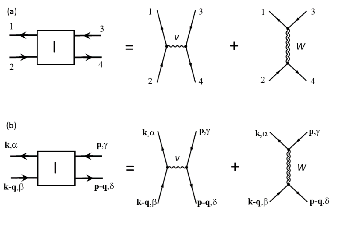
The instantaneous irreducible interaction $I$ contains, among many terms, an exchange-type electron-hole interaction of the form

$$I^{x}(\mbox{\boldmath$\xi$}_{1},\mbox{\boldmath$\xi$}_{2},\mbox{\boldmath$\xi$}_{3},\mbox{\boldmath$\xi$}_{4})=-i\delta(\mbox{\boldmath$\xi$}_{1}-\mbox{\boldmath$\xi$}_{2})\delta(\mbox{\boldmath$\xi$}_{3}-\mbox{\boldmath$\xi$}_{4})v(\mbox{\boldmath$\xi$}_{1}-\mbox{\boldmath$\xi$}_{3})\,$$

(32)

(see Fig. (4(a))). The Coulomb interaction can be separated into a long-range part

$$v_{lr}(\bm{\xi}-\bm{\xi}^{\prime})=\int_{BZ2}\frac{d^{2}{\bf q}}{(2\pi)^{2}}\frac{2\pi e^{2}}{q}e^{-q|z-z^{\prime}|}e^{i{\bf q}\cdot({\bf r}-{\bf r}^{\prime})}$$

(33)

where the integral runs over all values of $q_{z}$ and over ${\bf q}$ in the first Brillouin zone of the two-dimensional periodic lattice (BZ2), and a short-range part

$$\bar{v}(\bm{\xi}-\bm{\xi}^{\prime})=\sum_{{\bf G}\neq 0}\int_{BZ2}\frac{d^{2}{\bf q}}{(2\pi)^{2}}\frac{2\pi e^{2}}{|{\bf q}+{\bf G}|}e^{-|{\bf q}+{\bf G}||z-z^{\prime}|}e^{i({\bf q}+{\bf G})\cdot({\bf r}-{\bf r}^{\prime})}\,.$$

(34)

where the sum runs over all the two-dimensional reciprocal lattice vectors different from 0. The electron hole propagator $\bar{L}$, which enters Eq. (30), satisfies the same equation as $L$ (Eq. (31)), the only difference being that the long-range part of the interaction is excluded: only the short-range part, $\bar{v}$, is retained in $I^{x}$.

The BSE for $\bar{L}$ has the form

$$\begin{split}L(\mbox{\boldmath$\xi$}_{1},\mbox{\boldmath$\xi$}_{2},\mbox{\boldmath$\xi$}_{3},\mbox{\boldmath$\xi$}_{4};\omega)&=L_{0}(\mbox{\boldmath$\xi$}_{1},\mbox{\boldmath$\xi$}_{2},\mbox{\boldmath$\xi$}_{3},\mbox{\boldmath$\xi$}_{4};\omega)\\ &+\int d\mbox{\boldmath$\xi$}^{\prime}_{1}d\mbox{\boldmath$\xi$}^{\prime}_{2}d\mbox{\boldmath$\xi$}^{\prime}_{3}d\mbox{\boldmath$\xi$}^{\prime}_{4}L_{0}(\mbox{\boldmath$\xi$}_{1},\mbox{\boldmath$\xi$}_{2},\mbox{\boldmath$\xi$}_{1}^{\prime},\mbox{\boldmath$\xi$}_{2}^{\prime};\omega)\bar{I}(\mbox{\boldmath$\xi$}^{\prime}_{1},\mbox{\boldmath$\xi$}_{2}^{\prime},\mbox{\boldmath$\xi$}_{3}^{\prime},\mbox{\boldmath$\xi$}_{4}^{\prime})\bar{L}(\mbox{\boldmath$\xi$}_{3}^{\prime},\mbox{\boldmath$\xi$}_{4}^{\prime},\mbox{\boldmath$\xi$}_{3},\mbox{\boldmath$\xi$}_{4};\omega)\end{split}$$

(35)

where $\bar{I}$ is $I$ minus the long-range interaction term $I^{x}_{lr}(\mbox{\boldmath$\xi$}_{1},\mbox{\boldmath$\xi$}_{2},\mbox{\boldmath$\xi$}_{3},\mbox{\boldmath$\xi$}_{4})=-i\delta(\mbox{\boldmath$\xi$}_{1}-\mbox{\boldmath$\xi$}_{2})\delta(\mbox{\boldmath$\xi$}_{3}-\mbox{\boldmath$\xi$}_{4})v_{lr}(\mbox{\boldmath$\xi$}_{1}-\mbox{\boldmath$\xi$}_{3})$.

A further approximation that is commonly made at this point is to approximate the irreducible interaction as the sum of short-range exchange and direct terms (Fig. 4(a)):

$$\bar{I}(\mbox{\boldmath$\xi$}_{1},\mbox{\boldmath$\xi$}_{2},\mbox{\boldmath$\xi$}_{3},\mbox{\boldmath$\xi$}_{4})=\bar{I}^{x}(\mbox{\boldmath$\xi$}_{1},\mbox{\boldmath$\xi$}_{2},\mbox{\boldmath$\xi$}_{3},\mbox{\boldmath$\xi$}_{4})+\bar{I}^{d}(\mbox{\boldmath$\xi$}_{1},\mbox{\boldmath$\xi$}_{2},\mbox{\boldmath$\xi$}_{3},\mbox{\boldmath$\xi$}_{4})\,,$$

(36)

where

$$\bar{I}^{x}(\mbox{\boldmath$\xi$}_{1},\mbox{\boldmath$\xi$}_{2},\mbox{\boldmath$\xi$}_{3},\mbox{\boldmath$\xi$}_{4})=-i\delta(\mbox{\boldmath$\xi$}_{1}-\mbox{\boldmath$\xi$}_{2})\delta(\mbox{\boldmath$\xi$}_{3}-\mbox{\boldmath$\xi$}_{4})\bar{v}(\mbox{\boldmath$\xi$}_{1}-\mbox{\boldmath$\xi$}_{3})$$

(37)

and

$$\bar{I}^{d}(\mbox{\boldmath$\xi$}_{1},\mbox{\boldmath$\xi$}_{2},\mbox{\boldmath$\xi$}_{3},\mbox{\boldmath$\xi$}_{4})=\delta(\mbox{\boldmath$\xi$}_{1}-\mbox{\boldmath$\xi$}_{3})\delta(\mbox{\boldmath$\xi$}_{2}-\mbox{\boldmath$\xi$}_{4})W_{0}(\mbox{\boldmath$\xi$}_{1}-\mbox{\boldmath$\xi$}_{2},\omega=0)$$

(38)

where $W_{0}(\mbox{\boldmath$\xi$}_{1}-\mbox{\boldmath$\xi$}_{2},\omega=0)$ represents the statically screened Coulomb interaction.

The four-point functions are straightforwardly represented in our basis set. Taking as a prototype $L(\bm{\xi}_{1},\bm{\xi}_{2},\bm{\xi}_{3},\bm{\xi}_{4};\omega)$ we see that this is replaced by the matrix $L_{\alpha\beta,\gamma\delta}({\bf k},{\bf k}^{\prime},{\bf q};\omega)$ according to the scheme illustrated in the figure and analytically described by the equation

$$L(\bm{\xi}_{1},\bm{\xi}_{2},\bm{\xi}_{3},\bm{\xi}_{4};\omega)=\sum_{{\bf k},{\bf p},{\bf q}}\sum_{\alpha\beta\gamma\delta}\chi^{\alpha}_{{\bf k}}(\bm{\xi}_{1})[\chi^{\beta}_{{\bf k}-{\bf q}}(\bm{\xi}_{2})]^{*}L_{\alpha\beta,\gamma\delta}({\bf k},{\bf p},{\bf q};\omega)[\chi^{\gamma}_{{\bf p}}(\bm{\xi}_{3})]^{*}\chi^{\delta}_{{\bf p}-{\bf q}}(\bm{\xi}_{4})$$

(39)

where

$$L_{\alpha\beta,\gamma\delta}({\bf k},{\bf p},{\bf q};\omega)=\int d\bm{\xi}_{1}\bm{\xi}_{2}\bm{\xi}_{3}\bm{\xi}_{4}[\chi_{\alpha,{\bf k}}(\bm{\xi}_{1})]^{*}\chi_{\beta,{\bf k}-{\bf q}}(\bm{\xi}_{2})L(\bm{\xi}_{1},\bm{\xi}_{2},\bm{\xi}_{3},\bm{\xi}_{4};\omega)\chi_{\gamma,{\bf p}}(\bm{\xi}_{3})[\chi_{\delta,{\bf p}-{\bf q}}(\bm{\xi}_{4})]^{*}$$

(40)

In this basis, the BSE takes the form

	$\displaystyle L_{\alpha\beta,\gamma\delta}({\bf k},{\bf p},{\bf q};\omega)$	$\displaystyle=$	$\displaystyle L_{0(\alpha\beta,\gamma\delta)}({\bf k},{\bf p},{\bf q};\omega)$
		$\displaystyle+$	$\displaystyle\sum_{{\bf k}^{\prime}{\bf p}^{\prime}}\sum_{\alpha^{\prime}\beta^{\prime}\gamma^{\prime}\delta^{\prime}}L_{0,(\alpha\beta,\alpha^{\prime}\beta^{\prime})}({\bf k},{\bf k}^{\prime},{\bf q};\omega)I_{\alpha^{\prime}\beta^{\prime},\gamma^{\prime}\delta^{\prime}}({\bf k}^{\prime},{\bf p}^{\prime},{\bf q})L_{\gamma^{\prime}\delta^{\prime},\gamma\delta}({\bf p}^{\prime},{\bf p},{\bf q};\omega)\,.$

The noninteracting electron-hole propagator is given by

$$L_{0(\alpha\beta,\gamma\delta)}({\bf k},{\bf p},{\bf q};\omega)=~G_{0,\alpha\gamma}({\bf k},\omega)*G_{0,\delta\beta}({\bf k}-{\bf q},-\omega)\delta_{{\bf k},{\bf p}}\,.\$$

(42)

The frequency integral implied by the convolution product in this equation can be done analytically, with the help of the Kohn-Sham Green’s functions given in Eq. (15), the result being

$$L_{0(\alpha\beta,\gamma\delta)}({\bf k},{\bf p},{\bf q};\omega)=-i\delta_{{\bf k},{\bf p}}\sum_{n,m}\psi_{\alpha,n{\bf k}}\psi^{*}_{\gamma,n{\bf k}}\frac{f(E_{n{\bf k}})-f(E_{m{\bf k}-{\bf q}})}{\omega-E_{n{\bf k}}+E_{m{\bf k}-{\bf q}}\pm i0^{+}}\psi_{\beta,m{\bf k}}\psi^{*}_{\delta,m{\bf k}}\,,$$

(43)

where $E_{n{\bf k}}$ and $\psi^{\alpha}_{n{\bf k}}$ are, respectively, the Kohn-Sham energy and the Kohn-Sham wave function of the Bloch state $n{\bf k}$ in our representation, and $f(E_{n{\bf k}})$ is the Fermi-Dirac occupation factor of the same state. The two components of the irreducible four-point interaction function are (Fig. 4(b))

$$I^{x}_{\alpha\beta\gamma\delta}({\bf k},{\bf p},{\bf q})=-i\sum_{\mu\nu}\Gamma^{\mu}_{\alpha\beta}({\bf k},{\bf k}-{\bf q})v_{\mu\nu}({\bf q})\Gamma^{\nu}_{\delta\gamma}({\bf p}-{\bf q},{\bf p})$$

(44)

and

$$I^{d}_{\alpha\beta\gamma\delta}({\bf k},{\bf p},{\bf q})=\sum_{\mu\nu}\Gamma^{\mu}_{\alpha\gamma}({\bf k},{\bf p})w_{\mu\nu}({\bf k}-{\bf p})\Gamma^{\nu}_{\delta\beta}({\bf k}-{\bf q},{\bf p}-{\bf q})\,,$$

(45)

where the three-point vertices are defined by Eqs. (19) and  (20). Here $v_{\mu\nu}({\bf q})$ denotes the matrix elements of the Coulomb interaction in our basis set, i.e.,

$$v_{\mu\nu}({\bf q})=\int d\bm{\xi}\int d\bm{\xi}^{\prime}\chi^{*}_{\mu{\bf q}}(\bm{\xi})v(\bm{\xi}-\bm{\xi}^{\prime})\chi_{\nu{\bf q}}(\bm{\xi}^{\prime})$$

(46)

and similarly for $w_{\mu\nu}({\bf q})$, where $w\equiv W_{0}(\omega=0)$ is the statically screened interaction in the same basis. A similar expression holds for the regularized 4-point interaction $\bar{I}$ in terms of the regularized interaction $\bar{v}$, as previously discussed.

In this paper we have proposed that calculations of the electronic structure of quasi-two dimensional materials be performed on a native two-dimensional basis, consisting of two-dimensional Bloch sums of numerically generated atomic orbitals, such as the ones used in the AIMS-FHI approach. This approach removes the unphysical assumption of periodicity in the third dimension, which may be a cause of spurious results. The formal structure that we have developed in this paper lays the foundation for a direct two-dimensional numerical implementation of Kohn-Sham, GW, and Bethe-Salpeter equations in quasi 2D systems. We expect that the two-dimensional implementation of these tasks will speed up the calculations and make them more reliable, once the required computer codes are fully developed. While it may take a considerable initial effort to write the computer codes that will accomplish these tasks, we are confident that the payoff will be very high in the long run, resulting in a powerful computational tool occupying an intermediate position between those of molecular quantum chemistry and those of conventional solid state physics.

The authors thank A. H. Castro-Neto for his suggestions and support. PET gratefully acknowledges support from NRF under Grant No. R-723-000-001-281. GV gratefully acknowledges the hospitality of the Center for Advanced 2D Materials at NUS and support from DOE Grant No. DE-FG02-05ER46203.

References

- (1) K. S. Novoselov, A. K. Geim, S. V. Morozov, D. Jiang, Y. Zhang, S. V. Dubonos, I. V. Grigorieva, and A. A. Firsov. Electric Field Effect in Atomically Thin Carbon Films. Science, 306(5696):666–669, 2004.
- (2) A. Castro, H. Appel, M. Oliveira, C. A. Rozzi, X. Andrade, F. Lorenzen, M. A. L. Marques, E. K. U. Gross, and A. Rubio. Octopus: a tool for the application of time-dependent density functional theory. physica status solidi (b), 243(11):2465–2488, 2006.
- (3) J. Enkovaara, C. Rostgaard, J. J. Mortensen, J. Chen, M. Dułak, L. Ferrighi, J. Gavnholt, C. Glinsvad, V. Haikola, H. A. Hansen, H. H. Kristoffersen, M. Kuisma, A. H. Larsen, L. Lehtovaara, M. Ljungberg, O. Lopez-Acevedo, P. G. Moses, J. Ojanen, T. Olsen, V. Petzold, N. A. Romero, J. Stausholm-Møller, M. Strange, G. A. Tritsaris, M. Vanin, M. Walter, B. Hammer, H. Häkkinen, G. K. H. Madsen, R. M. Nieminen, J. K. Nørskov, M. Puska, T. T. Rantala, J. Schiøtz, and K. W. Jacobsen K. S. Thygesen and. Electronic structure calculations with GPAW: a real-space implementation of the projector augmented-wave method. Journal of Physics: Condensed Matter, 22(25):253202, 2010.
- (4) X. Gonze, B. Amadon, P.-M. Anglade, J.-M. Beuken, F. Bottin, P. Boulanger, F. Bruneval, D. Caliste, R. Caracas, M. Côté, T. Deutsch, L. Genovese, Ph. Ghosez, M. Giantomassi, S. Goedecker, D.R. Hamann, P. Hermet, F. Jollet, G. Jomard, S. Leroux, M. Mancini, S. Mazevet, M.J.T. Oliveira, G. Onida, Y. Pouillon, T. Rangel, G.-M. Rignanese, D. Sangalli, R. Shaltaf, M. Torrent, M.J. Verstraete, G. Zerah, and J.W. Zwanziger. Abinit: First-principles approach to material and nanosystem properties. Computer Physics Communications, 180(12):2582 – 2615, 2009.
- (5) P. Giannozzi, S. Baroni, N. Bonini, M. Calandra, R. Car, C. Cavazzoni, D. Ceresoli, G. L. Chiarotti, M. Cococcioni, I. Dabo, A. Dal Corso, S. de Gironcoli, S. Fabris, G. Fratesi, R. Gebauer, U. Gerstmann, C. Gougoussis, A. Kokalj, M. Lazzeri, L. Martin-Samos, N. Marzari, F. Mauri, R. Mazzarello, S. Paolini, A. Pasquarello, L. Paulatto, C. Sbraccia, S. Scandolo, G. Sclauzero, A. P. Seitsonen, A. Smogunov, P. Umari, and R. M. Wentzcovitch. QUANTUM ESPRESSO: a modular and open-source software project for quantum simulations of materials. Journal of Physics: Condensed Matter, 21(39):395502 (19pp), 2009.
- (6) G. Kresse and J. Furthmüller. Efficient iterative schemes for ab initio total-energy calculations using a plane-wave basis set. Phys. Rev. B, 54:11169–11186, 1996.
- (7) A. Gulans, S. Kontur, C. Meisenbichler, D. Nabok, P. Pavone, S. Rigamonti, S. Sagmeister, U. Werner, and C. Draxl. Exciting: a full-potential all-electron package implementing density-functional theory and many-body perturbation theory. Journal of Physics: Condensed Matter, 26(36):363202, 2014.
- (8) http://elk.sourceforge.net/.
- (9) C. Friedrich, S. Blügel, and A. Schindlmayr. Efficient implementation of the approximation within the all-electron FLAPW method. Phys. Rev. B, 81:125102, 2010.
- (10) M. Methfessel, M. van Schilfgaarde, and R. A. Casali. ”A full-potential LMTO method based on smooth Hankel functions”, Electronic Structure and Physical Properties of Solids: The Uses of the LMTO Method, Lecture Notes in Physics, volume 535. Springer-Verlag, Berlin, 2000.
- (11) V. Blum, R. Gehrke, F. Hanke, P. Havu, V. Havu, X. Ren, K. Reuter, and M. Scheffler. Ab initio molecular simulations with numeric atom-centered orbitals. Computer Physics Communications, 180(11):2175–2196, 2009.
- (12) J. M. Soler, E. Artacho, J. D. Gale, A. García, J. Junquera, P. Ordejón, and D. Sánchez-Portal. The SIESTA method for ab initio order- N materials simulation. Journal of Physics: Condensed Matter, 14(11):2745, 2002.
- (13) P. Cudazzo, I. V. Tokatly, and A. Rubio. Dielectric screening in two-dimensional insulators: Implications for excitonic and impurity states in graphane. Phys. Rev. B, 84:085406, 2011.
- (14) S. Latini, T. Olsen, and K. S. Thygesen. Excitons in van der Waals heterostructures: The important role of dielectric screening. Phys. Rev. B, 92:245123, Dec 2015.
- (15) N. D. Lang and W. Kohn. Theory of metal surfaces: Charge density and surface energy. Phys. Rev. B, 1:4555–4568, Jun 1970.
- (16) C.-O. Almbladh and U. von Barth. Exact results for the charge and spin densities, exchange-correlation potentials, and density-functional eigenvalues. Phys. Rev. B, 31:3231–3244, Mar 1985.
- (17) V. M. Silkin, J. Zhao, F. Guinea, E. V. Chulkov, P. M. Echenique, and H. Petek. Image potential states in graphene. Phys. Rev. B, 80:121408, Sep 2009.
- (18) C. A. Rozzi, D. Varsano, A. Marini, E. K. U. Gross, and A. Rubio. Exact Coulomb cutoff technique for supercell calculations. Physical Review B, 73(20):205119, 2006.
- (19) A. Castro, E. Räsänen, and C. A. Rozzi. Exact Coulomb cutoff technique for supercell calculations in two dimensions. Physical Review B, 80(3):033102, 2009.
- (20) V. U. Nazarov. Electronic excitations in quasi-2D crystals: what theoretical quantities are relevant to experiment? New Journal of Physics, 17(7):073018, 2015.
- (21) Lin-Hui Ye. Surface calculations with asymptotically long-ranged potentials in the full-potential linearized augmented plane-wave method. Phys. Rev. B, 92:115132, 2015.
- (22) Zhang I. Y., Ren X., Rinke P., Blum V., and Scheffler M. Numeric atom-centered-orbital basis sets with valence-correlation consistency from H to Ar. New Journal of Physics, 15(12):123033, 2013.
- (23) X. Ren, P. Rinke, V. Blum, J. Wieferink, A. Tkatchenko, A. Sanfilippo, K. Reuter, and M. Scheffler. Resolution-of-identity approach to Hartree–Fock, hybrid density functionals, RPA, MP2 and GW with numeric atom-centered orbital basis functions. New Journal of Physics, 14(5):053020, 2012.
- (24) F. Giustino, M. L. Cohen, and S. G. Louie. GW method with the self-consistent Sternheimer equation. Phys. Rev. B, 81:115105, 2010.
- (25) H. Lambert and F. Giustino. Ab initio Sternheimer-GW method for quasiparticle calculations using plane waves. Phys. Rev. B, 88:075117, 2013.
- (26) M. Rohlfing, P. Krüger, and J. Pollmann. Quasiparticle band-structure calculations for C, Si, Ge, GaAs, and SiC using Gaussian-orbital basis sets. Phys. Rev. B, 48:17791–17805, 1993.
- (27) M. Rohlfing, P. Krüger, and J. Pollmann. Quasiparticle Band Structure of CdS. Phys. Rev. Lett., 75:3489–3492, 1995.
- (28) M. Rohlfing and S. G. Louie. Electron-hole excitations and optical spectra from first principles. Phys. Rev. B, 62:4927–4944, 2000.
- (29) G. Onida, L. Reining, and A. Rubio. Electronic excitations: density-functional versus many-body Green’s-function approaches. Reviews of Modern Physics, 74(2):601–659, 2002.
- (30) P. Romaniello, D. Sangalli, J. A. Berger, F. Sottile, L. G. Molinari, L. Reining, and G. Onida. Double excitations in finite systems. The Journal of Chemical Physics, 130(4), 2009.
- (31) G. Strinati. Effects of dynamical screening on resonances at inner-shell thresholds in semiconductors. Phys. Rev. B, 29:5718–5726, 1984.
- (32) M. E. Casida. Recent Advances in Density functional Methods, volume 1, chapter Time Dependent functional response theory for molecules. World scientific, Singapore, 1995.
- (33) M. S. Hybertsen and S. G. Louie. First-Principles Theory of Quasiparticles: Calculation of Band Gaps in Semiconductors and Insulators. Phys. Rev. Lett., 55:1418–1421, 1985.
- (34) E. L. Shirley and R. M. Martin. GW quasiparticle calculations in atoms. Phys. Rev. B, 47:15404–15412, 1993.
- (35) D. L. Johnson. Local field effects and the dielectric response matrix of insulators: A model. Phys. Rev. B, 9:4475–4484, 1974.
- (36) S. Lebègue, B. Arnaud, M. Alouani, and P. E. Bloechl. Implementation of an all-electron GW approximation based on the projector augmented wave method without plasmon pole approximation: Application to Si, SiC, AlAs, InAs, NaH, and KH. Phys. Rev. B, 67:155208, 2003.