Mean-Field-Type Games in Engineering

Boualem Djehiche Alain Tcheukam Hamidou Tembine ^†^†thanks: B. Djehiche is with Department of Mathematics, KTH Royal Institute of Technology, Stockholm, Sweden ^†^†thanks: A. Tcheukam and H. Tembine are with Learning and Game Theory Lab, New York University Abu Dhabi. Email: tembine@nyu.edu

Abstract

A mean-field-type game is a game in which the instantaneous payoffs and/or the state dynamics functions involve not only the state and the action profile but also the joint distributions of state-action pairs.This article presents engineering applications of mean-field-type games.

Keywords: mean-field-type game, electrical, computer, mechanical, civil, general engineering

1 Introduction

With the ever increasing amounts of data becoming available, strategic data analysis and decision-making will become more pervasive as a necessary ingredient for societal infrastructures. In many network engineering games, the performance metrics depend on some few aggregates of the parameters/choices. A typical example is the congestion field in traffic engineering where classical cars and smart autonomous driverless cars create traffic congestion levels on the roads. The congestion field can be learned, for example by means of crowdsensing, and can be used for efficient and accurate prediction of the end-to-end delays of commuters. Another example is the interference field where it is the aggregate-received signal of the other users that matters rather than their individual input signal. In such games, in order for a transmitter-receiver pair to determine his best-replies, it is unnecessary that the pair is informed about the other users’ strategies. If a user is informed about the aggregative terms given her own strategy, she will be able to efficiently exploit such information to perform better. In these situations the outcome is influenced not only by the state-action profile but also by the distribution of it. The interaction can be captured by a game with distribution-dependent payoffs called mean-field-type games (MFTG). An MFTG is basically a game in which the instantaneous payoffs and/or the state dynamics functions involve not only the state and the action profile of the agents but also the joint distributions of state-action pairs.

The main contributions of this article can be summarized as follows. The first contribution of this article is the review of some relevant engineering applications of MFTG. Considering Liouville type systems with drift, diffusion and jumps, that are dependent on time-delays, state mean-field and action mean-field terms. Proposition 7 establishes an equilibrium equation for non-convex action spaces. Proposition 9 provides a stochastic maximum principle that covers decentralized information and partial observation systems which are crucial in engineering systems. Various engineering applications in discrete or continuous variables (state, action or time) are provided. Explicit solutions are provided in propositions 6 and 8 which are mean-field type game problems with non-quadratic costs.

The article is structured as follows. The next section overviews earlier works on static mean-field games, followed by discrete time mean-field games with measure-dependent transition kernels. Then, a basic MFTG with finite number of agents is presented. After that, the discussion is divided into two illustrations in each of the following areas of engineering (Figure 1) : Civil Engineering (CE), Electrical Engineering (EE), Computer Engineering (CompE), Mechanical Engineering (ME), General Engineering (GE).

•

CE: road traffic networks with random incident states and multi-level building evacuation
•

EE: Millimeter wave wireless communications and distributed power networks
•

CompE: Virus spread over networks and virtual machine resource management in cloud networks
•

ME: Synchronization of oscillators, consensus, alignment and energy-efficient buildings
•

GE: Online meeting: strategic arrivals and starting time and mobile crowdsensing as a public good.

The article proceeds by presenting the effect of time delays of coupled mean-field dynamical systems and decentralized information structure. Then, a discussion on the drawbacks, limitations, and challenges of MFTGs is highlighted. Lastly, a summary of the article and concluding remarks are presented.

Refer to caption — Figure 1: MFTG with engineering applications covered in this work.

1.1 Mean-Field Games: Static Setup

A static mean-field game is one in which all users make choices (or select a strategy) simultaneously, without knowledge of the strategies that are being chosen by other users and the game is played once. Any mean-field game with sequential moves is a dynamic mean-field game. In this work, games which are played more than once will be considered as dynamic game. This subsection overviews static mean-field games and games in which the underlying processes are in stationary regime (time-independent). Mean-field games have been around for quite some time in one form or another, especially in transportation networks and in competitive economy. In the context of competitive market with large number of agents, a 1936 article [1] captures the assumption made in mean-field games with large number of agents, in which the author states:

“each of the participants has the opinion that its own actions do not influence the prevailing price”.

Another comment on the impact on the population mean-field term was given in [2] page 13:

“ When the number of participants becomes large, some hope emerges that of the influence of every particular participant will become negligible …”

The population interaction involves many agents for each type or class and location, a common approach is to replace the individual agents’ variables and to use continuous variables to represent the aggregate average of type-location-actions. In the large population regime, the mean field limit is then modeled by state-action and location-dependent time process (see Figure 2). This type of aggregate models are also known as non-atomic or population games. It is closely related to the mass-action interpretation in [3], Equation (4) in page 287.

In the context of transportation networks, the mean-field game framework, underlying the key foundation, goes back to the pioneering works of [4] in the 1950s. Therein, the basic idea is to describe and understand interacting traffic flows among a large population of agents moving from multiple sources to destinations, and interacting with each other. The congestion created on the road and at the intersection are subject to capacity and flow constraints. This corresponds to a constrained mean-field game problem as noted in [5]. A common behavioral assumption in the study of transportation and communication networks is that travelers or packets, respectively, choose routes that they perceive as being the shortest under the prevailing traffic conditions. As noted in [6], collection of individual decisions may result to a situation which drivers cannot reduce their journey times by unilaterally choosing another route. The work in [6] such a resulting traffic pattern as an equilibrium. Nowadays, it is indeed known as the Wardrop equilibrium [4, 7], and it is thought of as a steady state obtained after a transient phase in which travelers successively adjust their route choices until a situation with stable route travel costs and route flows has been reached [8, 9]. In the seminal contribution [4], page 345 the author stated two principles that formalize this notion of equilibrium and the alternative postulates of the minimization of the total travel costs. His first principle reads:

“The journey times on all the routes actually used are equal, and less than those which would be experienced by a single vehicle on any unused route.”

Wardrop’s first principle of route choice, which is identical to the notion postulated in [10, 6], became widely used as a sound and simple behavioral principle to describe the spreading of trips over alternate routes due to congested conditions. Since its introduction in the context of transportation networks in 1952 and its mathematical formalization by [5, 11] transportation planners have been using Wardrop equilibrium models to predict commuters decisions in real-life networks.

The key congestion factor is the flow or the fraction of travelers per edge on the roads (see Application 1). The above Wardrop problem is indeed a mean-field on a discrete space. The exact mean-field term here corresponds to a mean-field of actions (a choice of a route). Putting this in the context of infinite number of commuters results to end-to-end travel times that are function of own choice of a route and the mean-field distribution of travelers across the graph (network).

In a population context, the equilibrium concept of [4] corresponds to a Nash equilibrium of the mean-field game with infinite number of agents. The works [7, 12] provide a variational formulation of the (static) mean-field equilibrium.

The game theoretic models such as evolutionary games [13, 14, 15], global games [16, 17], anonymous games, aggregative games [18], population games [19, 20, 21], and large games, share several common features. Static mean-field games with large number of agents were widely investigated (see [22, 23, 24, 25, 26, 27] and the references therein).

1.2 Mean-Field Games: Dynamic Setup

This section overviews mean-field games which are dynamic (time-varying and played more than once) and their applications in engineering.

Definition 1 (Mean-Field Game: Infinite Regime).

A (homogeneous population) mean-field game (MFG) is a game in which the instantaneous payoff of a generic agent (say 1) and/or the state dynamics coefficient functions involve an individual state-action pair $x_{1t},u_{1t}$ and the distribution of state-action pairs of the other decision-makers, $m_{t}$ at time $t.$ The individual state and action spaces are identical across the homogeneous population denoted by $\mathcal{X}_{i}=\mathcal{X}_{1},U_{j}=U_{1}$ for all $i.$ The state transition to the next state follows $\mathbb{P}(.|x_{1t},u_{1t},m_{t}).$ Thus, the instant payoff function of a generic agent (say $j$ ) has the following structure:

r_{i}=r_{1}=r:\ \mathcal{X}_{1}\times U_{1}\times\mathbb{P}(\mathcal{X}_{1}\times U_{1})\rightarrow\mathbb{R},

with $r(x_{1t},u_{1t},m_{t}).$

The mean-field game model has been extended to include several other features such as incomplete information, common noise, heterogeneous population, finite population or a mixture between finite number of clusters and infinite population regimes.

The key ingredients of dynamic mean-field games appeared in [28, 29] in the early 1980s. The work in [28] proposes a game-theoretic model that explains why smaller firms grow faster and are more likely to fail than larger firms in large economies. The game is played over a discrete time space. Therein, the mean-field is the aggregate demand/supply which generates a price dynamics. The price moves forwardly, and the agents react to the price and generate a demand and the firm produces a supply with associated cost, which regenerates the next price and so on. The author introduced a backward-forward system to find equilibria (see for example Section 4, equations D.1 and D.2 in [28]). The backward equation is obtained as an optimality to the individual response, i.e., the value function associated with the best response to price, and the forward equation for the evolution of price. Therein, the consistency check is about the mean-field of equilibrium actions (population or mass of actions), that is, the equilibrium price solves a fixed-point system: the price regenerated after the reaction of the agents through their individual best-responses should be consistent with the price they responded to.

Following that analogy, a more general framework was developed in [29], where the mean-field equilibrium is introduced in the context of dynamic games with large number of decision-makers. A mean-field equilibrium is defined in [29], page 80 by two conditions: (1) each generic agent’s action is best-response to the mean-field, and (2) the mean-field is consistent and is exactly reproduced from the reactions of the agents. This matching argument was widely used in the literature as it can be interpreted as a generic agent reacting to an evolving mean-field object and at the same time the mean-field is formed from the contributions of all the agents. The authors of [30] show how common noise can be introduced into the mean-field game model (the mean-field distribution evolves stochastically) and extend the Jovanovic-Rosenthal existence theorem [29].

Continuous time version of the works [28, 29] can be found in [31, 32, 33, 34]. The reader is referred to [36, 37, 38, 42, 39, 40, 41] for recent development of mean-field game theory. The authors [43, 44, 33, 45, 46, 47] have developed a powerful tool for modelling strategic behavior of large population of agents, each of them having a negligible impact on the population mean-field term. Weak solutions of mean-field games are analyzed in [48], Markov jumps processes [49, 50], and leader-followers models in [51]. Finite state mean-field game models were analyzed in [52, 53, 54, 55, 56, 57, 58, 59]. Team and social optimum solutions can be found in [60, 61, 62, 51, 63]. The work in [64, 65, 66] provide mean-field convergence of a class of McKean-Vlasov dynamics. Numerical methods for mean-field games can be found in [67, 68, 69, 70].

Table 1 summarizes some engineering applications of mean-field-type game models.

Table 1: Some applications of MFTGs in Engineering. HVAC stands for (heating, ventilation and air conditioning) systems. D2D stands for Device-to-Device (D2D)

Area	Works
planning	[72]
state estimation and filtering	[73, 74]
synchronization	[75, 76, 77, 78]
opinion formation	[79]
network security	[80, 81, 82, 83, 84]
power control	[85, 86, 87]
medium access control	[88, 89]
cognitive radio networks	[90, 91]
electrical vehicles	[92, 93]
scheduling	[94]
cloud networks	[95, 96, 97]
wireless networks	[98]
auction	[99, 100]
cyber-physical systems	[101, 102]
airline networks	[103]
sensor networks	[104]
traffic networks	[105, 106, 107, 108]
big data	[109]
D2D networks	[110, 111, 112]
multilevel building evacuation	[140, 141, 142, 143]
power networks	[113, 114, 115, 116, 117, 174, 179]
	[118, 119, 120, 93, 121]
	[122, 123, 124]
HVAC	[125, 126, 127, 128, 129, 130]

1.2.1 Limitations of the existing mean-field game models

Most of the existing mean-field game models share the following assumptions:

Big size: A typical assumption is to consider an infinite number decision-makers, sometimes, a continuum of decision-makers. The idea of a continuum of decision-makers may seem outlandish to the reader. Actually, it is no stranger than a continuum of particles used in fluid mechanics, in water distribution, or in petroleum engineering. In terms of practice and experiment however, decision-making problems with continuum of decision-makers is rarely observed in engineering. There is a huge difference between a fluid with a continuum of particles and a decision-making problem with a continuum of agents. Agents may physically occupy a space (think of agents inside a building or a stadium) or a resource, and the size or number of agents that most of engineering systems can handle can be relatively large or growing but remain currently finite [71]. It is in part due to the limited resource per shot or limited number of servers at a time. In all the examples and applications provided below, we still have a finite number of interacting agents. Thus, this assumption appears to be very restrictive in terms of engineering applications.

Anonymity: The index of the decision-maker does not affect the utility. The agents are assumed to be indistinguishable within the same class or type. The drawback of this assumption is that most individual decision-makers in engineering are in fact not necessarily anonymous (think of Google, Microsoft, Twitter, Facebook, Tesla), the classical mean-field game model is inappropriate, and does not apply to such situations. In mean-field games with several types (or multi-population mean-field games), it is still assumed that there is large number of agents per type/class/population, which is not realistic in most of the engineering applications considered in this work.

NonAtomicity: A single decision-maker has a negligible effect on the mean-field-term and on the global utility. One typical example where this assumption is not satisfied is a situation of targeting a room comfort temperature, in which the air conditioning controller adjusts the heating/cooling depending on the temperature in the room, the temperatures of the other connecting zones and the ambient temperature. It is clear that the decision of the controller to heat or to cool affect the variance of the temperature inside the room. Thus, the effect of the individual action of that controller on the temperature distribution (mean-field) inside the room cannot be neglected.

To summarize, the above conditions appear to be very restrictive in terms of engineering applications, and to overcome this issue a more flexible MFTG framework has been proposed.

1.2.2 What MFTGs can bring to the existing decision-making models?

MFTGs not only relax of the above assumptions but also incorporate the behavior of the agents as well as their effects in the mean-field terms and in the outcomes (see Table 2).

(1)

In MFTGs, the number of users can be finite or infinite.
(2)

The indistinguishability property (invariance in law by permutation of index of the users) is not assumed in MFTGs.
(3)

A single user may have a non-negligible impact of the mean-field terms, specially in the distribution of own-states and own mixed strategies.

These properties (1)-(3) make strong differences between mean-field games and MFTGs (see [132] and the references therein).

Table 2: Key limitations and differences between the game models

Area	Anonymity	Infinity	Atom
population games [4, 5]	yes	yes	no
evolutionary games [131]	yes	yes	no
non-atomic games [29]	yes	yes	no
aggregative games [18]		relaxed
global games [16, 17]	yes	yes	no
large games [22]	yes	yes	no
anonymous games [29]	yes	yes	no
mean-field games	yes	yes	no
nonasymptotic mean-field games	nearly	no	yes
MFTG	relaxed	relaxed	relaxed

MFTG seems to be more appropriate in such engineering situations because it does not assume indistinguishability, it captures the effect of each agent in the distribution and the number of agents is arbitrary as we will see below. Table 3 summarizes the notations used in the manuscript.

Table 3: Table of Notations

$\mathcal{I}$	$\triangleq$	set of decision-makers
$T$	$\triangleq$	Length of the horizon
$[0,T]$	$\triangleq$	horizon of the mean-field-type game
$t$	$\triangleq$	time index
$\mathcal{X}$	$\triangleq$	state space
$W$	$\triangleq$	Brownian motion
$\sigma$	$\triangleq$	Diffusion coefiicient
$N$	$\triangleq$	Poisson jump process
$\gamma$	$\triangleq$	Jump rate coefiicient
${U}_{i}$	$\triangleq$	control action space of agent $i\in\mathcal{I}$
$\mathcal{U}_{i}$	$\triangleq$	admissible strategy space
$u_{i}$	$\triangleq$	state space
$r_{i}$	$\triangleq$	instantaneous payoff
$D_{(x,u)}$	$\triangleq$	distribution of state-action
$R_{i}$	$\triangleq$	Long-term payoff functional

1.3 Background on MFTGs

This section presents a background on MFTGs.

Definition 2 (Mean-Field-Type Game).

A mean-field-type game (MFTG) is a game in which the instantaneous payoffs and/or the state dynamics coefficient functions involve not only the state and the action profile but also the joint distributions of state-action pairs (or its marginal distributions, i.e., the distributions of states or the distribution of actions). Let $\mathcal{I}$ be the set of agents, $\mathcal{X}_{i}$ the state space of agent $i$ and $\mathcal{X}:=\prod_{i\in\mathcal{I}}\mathcal{X}_{i}=\mathcal{X}_{1}\times\mathcal{X}_{2}\times\ldots$ the state profiles space of all agents. $U_{i}$ is the action space of agent $i$ and $U=\prod_{j}U_{j}$ is the action profile space of all agents. A typical example of payoff function of agent $j$ has the following structure:

r_{i}:\ \mathcal{X}\times U\times\mathbb{P}(\mathcal{X}\times U)\rightarrow\mathbb{R},

with $r_{i}(x,u,D_{(x,u)})$ where $(x,u)$ is the state-action profile of the agents and $D_{(x,u)}$ is the distribution of the state-action pair $(x,u).$ $\mathcal{X}$ is the state space, $U$ is the action profile space of all agents and $\mathbb{P}(\mathcal{X}\times U)$ is the set of probability measures over $\mathcal{X}\times U.$

From Definition 2, a mean-field-type game can be static or dynamic in time. One may think that MFTG is a small and particular class of games. However, this class includes the classical games in strategic form because any payoff function $r_{i}(x,u)$ can be written as $r_{i}(x,u,D).$

When randomized/mixed strategies are used in the von Neumann-type payoff, the resulting payoff can be written as $E[r_{i}(x,u)]=\int r_{i}(x,u)D_{(x,u)}(dx,du)=\hat{r}_{i}(D).$ Thus, the form $r_{i}(x,u,D)$ is more general and includes non-von Neumann payoff functions.

Example 1 (Mean-variance payoff).

The payoff function of agent $i$ is $E[r_{i}(x,u)]-\lambda\sqrt{var[r_{i}(x,u)]},\lambda\in\mathbb{R}$ which can be written as a function of $r_{i}(x,u,D_{(x,u)}).$ For any number of interacting agents, the term $D_{(x_{i},u_{i})}$ plays a non-negligible role in the standard deviation $\sqrt{var[r_{i}(x,u)]}.$ Therefore, the impact of agent $i$ in the individual mean-field term $D_{(x_{i},u_{i})}$ cannot be neglected.

Example 2 (Aggregative games).

The payoff function of each agent depends on its own action and an aggregative term of the other actions. Example of payoff functions include $r_{i}(u_{i},\sum_{j\neq i}u^{\alpha}_{j}),\ \alpha>0$ and $r_{i}(x_{i}u_{i},\sum_{j\neq i}x_{j}u_{j}).$

In the non-atomic setting, the influence of an individual state $x_{i}$ and individual action $u_{i}$ of any agent $i$ will have a negligible impact on mean-field term $\hat{D}_{(x,u)}=\lim_{n\rightarrow+\infty}\ \frac{1}{n-1}\sum_{j\neq i}\delta_{\{x_{j},u_{j}\}}.$ In that case, one gets to the so-called mean-field game.

Example 3 (Population games).

Consider a large population of agents. Each agent has a certain state/type $x\in\mathcal{X}$ and can choose a control action $u\in\mathcal{U}(x).$ Let the proportion of type-action of the population as $m.$ The payoff of the agent with type/state $x,$ control action $u$ when the population profile $m$ is $r(x,u,m).$ Global games with continuum of agents were studied in [16] based on the Bayesian games of [17], which uses the proportion of actions.

In the case where both non-atomic and atomic terms are involved in the payoff, one can write the payoff as $r_{i}(x,u,D,\hat{D})$ where $\hat{D}$ is the population state-action measure. Agent $i$ may influence $D_{i}$ (distribution of its own state-action pairs) but its influence on $\hat{D}$ may be limited.

The main goals of static mean-field-type games are: (1) identify solution concepts [35] such as Nash equilibrium, Bayesian equilibrium, correlated equilibrium, Stackelberg solution etc. (2) Computation of solution concepts. (3) Development of algorithms and learning procedures to reach and select efficient equilibria, (4) Mechanism design for incentivizing agents. The next section presents a class of dynamic MFTGs which are played over several stages.

2 A Basic Dynamic MFTG: Finite Regime

Consider a basic MFTG with $n\geq 2$ agents interacting over horizon $[0,T],\ \ T>0.$ The individual state dynamics of agent $i$ is given by

\begin{array}[]{ll}dx_{i}=b_{i}\left(x_{i},u_{i},D_{(x_{i},u_{i})},\frac{\sum_{k\neq i}\delta_{(x_{k},u_{k})}}{n-1}\right)dt+\sigma_{i}\left(x_{i},u_{i},D_{(x_{i},u_{i})},\frac{\sum_{k\neq i}\delta_{(x_{k},u_{k})}}{n-1}\right)dW_{i},\\ x_{i}(0)\sim D_{i,0}\end{array}

(1)

and the payoff functional of agent $i$ is

\displaystyle R_{i}(u)=g_{i}\left(x_{i}(T),D_{x_{i}(T)},\frac{\sum_{k\neq i}\delta_{x_{k}(T)}}{n-1}\right)+\int_{0}^{T}r_{i}\left(x_{i},u_{i},D_{(x_{i},u_{i})},\frac{\sum_{k\neq i}\delta_{(x_{k},u_{k})}}{n-1}\right)dt,

(2)

where the strategy profile is $u=(u_{1},\ldots,u_{n}),$ which also denoted as $(u_{i},u_{-i}).$ The functions $b_{i},\sigma_{i},g_{i},r_{i}$ are measurable functions. $x_{i}(t):=x_{i}(t)[u]$ is the state of agents $i$ under of the strategy profile $u,$ $D_{x_{i}(t)}=\mathcal{L}(x_{i}(t))$ is the probability distribution (law) of $x_{i}(t).$ $D_{(x_{i}(t),u_{i}(t))}=\mathcal{L}(x_{i}(t),u_{i}(t))$ is the probability distribution of the state-control action pair $(x_{i}(t),u_{i}(t))$ of agent $i$ at time $t.$ $\delta_{y}$ is the $\delta-$ Dirac measure concentrated at $y,$ and $W_{i}$ is a standard Brownian motion defined over the filtration $(\Omega,\mathbb{P},(\mathcal{F}_{t})_{t\leq T}).$

The novelty in the modelling of (1)-(2) is that each individual agent $i$ influences its own mean-field terms $D_{x_{i}(t)},$ and $D_{(x_{i}(t),u_{i}(t))}$ independently on the total number of interacting agents. In particular, the influence of agent $i$ on those mean-field terms remain non-negligible even when there is a continuum of agents. The distributions $D_{x_{i}}$ and $D_{(x_{i},u_{i})}$ represent two important terms in the modeling of MFTGs. These terms are referred to as individual mean-field terms. In the finite regime, the other agents are captured by the empirical measures $\frac{\sum_{k\neq i}\delta_{x_{k}}}{n-1}$ and $\frac{\sum_{k\neq i}\delta_{(x_{k},u_{k})}}{n-1}.$ We refer these terms to as population mean-field terms.

Similarly, a basic discrete time (discrete or continuous state) MFTG is given by

\begin{array}[]{ll}x_{i,t+1}\sim q_{i}\left(.|x_{i,t},u_{i,t},D_{(x_{i,t},u_{i,t})},\frac{\sum_{k\neq i}\delta_{(x_{k,t},u_{k,t})}}{n-1}\right),\\ x_{i0}\sim D_{i,0}\\ R_{i}(u)=g_{i}\left(x_{i,T},D_{x_{i,T}},\frac{\sum_{k\neq i}\delta_{x_{k,T}}}{n-1}\right)+\sum_{t=0}^{T-1}r_{i}\left(x_{i,t},u_{i,t},D_{(x_{i,t},u_{i,t})},\frac{\sum_{k\neq i}\delta_{(x_{k,t},u_{k,t})}}{n-1}\right),\end{array}

(3)

where $q_{i}(.|.)$ is the transition kernel of agent $i$ to next states.

Mean-field-type control and global optimization can be found in [134, 36, 133, 172, 173, 175]. The models (1) and (3) are easily adapted to bargaining solution, cooperative and coalitional MFTGs and can be found in [135, 176, 177]. Psychological MFTG was recently introduced in [111, 178] where spitefulness, altruism, selfishness, reciprocity of the agents are examined by means empathy, other-regarding behavior and psychological factors.

Definition 3.

An admissible control strategy of agent $i$ is an $\mathcal{F}_{i}-$ adapted and square integrable process with values in a non-empty subset ${U}_{i}.$ Denote by $\mathcal{U}_{i}=L^{2}_{\mathcal{F}_{i}}([0,T],\ U_{i})$ the class of admissible control strategies of agent $i$ .

Definition 4 (Best response).

Given a strategy profile of the other agents $(u_{1},\ldots,u_{i-1},u_{i+1},\ldots,u_{n}),$ with $u_{j},\ j\neq i$ that are admissible and the mean-field terms $D$ , the best response problem of agent $i$ is:

\displaystyle\left\{\begin{array}[]{l}\displaystyle{\sup_{u_{i}\in\mathcal{U}_{i}}\mathbb{E}\left[R_{i}(u)\right]},\\ \mbox{subject to}\ (\ref{eq:state})\end{array}\right.

The first goal is to find and characterize the best response strategies of each user. For user $i$ it consists to solve problem (4). In problem (4), the information structure that is available to user plays in important role. We will distinguish three type of strategies: (1) open-loop strategies that are only measurable function of $t,$ (2) state-feedback strategies that are measurable functions of state and time, (3) state-and-mean-field feedback strategies that measurable functions of state, mean-field and time. To solve problem (4), four different methods have been developed:

•

Direct approach which consists to write the payoff functional in a form such that the optimal value and optimizers are trivially obtained, and a verification and validation procedure follows.
•

A stochastic maximum principle (Pontryagin’s approach) which provides necessary conditions for optimality.
•

A dynamic programming principle (Bellman’s approach) which consists to write the value of the problem (per agent) in (backward) recursion form, or as solution to a dynamical system.
•

Uncertainty quantification approach by means of Wiener chaos expansion of all the stochastic terms and the use of Kosambi-Karhunen-Loeve expansion which is a representation of a stochastic process as an infinite linear combination of orthogonal functions, analogous to a Fourier series representation of a function over a bounded domain.

If every user solves its best-response problem, the resulting system will be a Nash equilibrium system defined below.

Definition 5.

A (Nash) equilibrium of the game is a strategy profile $(u^{*}_{1},\ldots,u^{*}_{n})$ such that for every agent $i$ ,

\mathbb{E}[R_{i}(u^{*})]\geq\mathbb{E}[R_{i}(u^{*}_{1},\ldots,u_{i-1}^{*},u_{i},u_{i+1}^{*},\ldots,u^{*}_{n})],

for all $u_{i}\in\mathcal{U}_{i}.$

The second goal is to find and characterize Nash equilibria of the mean-field-type game. We provide below a basic example in which the Nash equilibrium problem can be solved semi-explicitly using Riccati system.

Example 4 (Network Security Investment [80] ).

A graph is connected if there is a path that joins any point to any other point in the graph. Consider $n\geq 2$ decision-makers over a connected graph. Thus, the security of a node is influenced by the others through possibly multiple hops. The effort of user $i$ in security investment is $u_{i}.$ The associated cost may include money (e.g., for purchasing antivirus software), time and energy (e.g., for system scanning, patching). Let $x(t)$ be the security level of the network at time $t$ and

\begin{array}[]{lll}R_{i}(u)=\ \ -\frac{1}{2}[x(T)-Ex(T)]^{2}+\int_{0}^{T}q_{i}(t)x(t)(1-\epsilon_{i}(t)x(t))-\rho_{i}(t)u_{i}(t)-\frac{r_{i}(t)}{2}u^{2}_{i}(t)dt.\end{array}

(7)

The best-response of user $i$ to $(u_{-i},E[x]):=(u_{1},\ldots,u_{i-1},u_{i+1},\ldots,u_{n},E[x]),$ solves the following linear-quadratic mean-field-type control problem

\displaystyle\left\{\begin{array}[]{lll}\sup_{u_{i}\in\mathcal{U}_{i}}E\left[R_{i}(u_{1},\ldots,u_{n})\right],\ \displaystyle{\mbox{ subject to }\ }\\ dx=\left\{-ax-\bar{a}E[x]+\sum_{i=1}^{n}b_{i}u_{i}\right\}dt+cxdW,\\ x(0)\in\mathbb{R},\end{array}\right.

where, $q_{i}(t)\geq 0,\epsilon_{i}(t)\geq 0,\rho_{i}(t)\geq 0,\ r_{i}(t)>0$ and $a,\bar{a},b_{i},c$ are real numbers and where $E[x(t)]$ is the expected value of network security level created by all users under the control action profile $(u_{1},\ldots,u_{n}).$ Note that the expected value of the terminal term in $R_{i}$ can be seen as a weighted variance of the state [130] since $E[(x(t)-E[x(t)])^{2}]=var(x(t)).$ The optimal control action is in state-and-mean-field feedback form:

\begin{array}[]{ll}u^{*}_{i}(t)=-\frac{b_{i}}{r_{i}(t)}\left[\beta_{i}(t)x(t)+\eta_{1i}(t)E[x(t)]+\eta_{2i}(t)\right]-\frac{\rho_{i}(t)}{r_{i}(t)},\\ 0=\dot{\beta}_{i}+(-2a+c^{2})\beta_{i}-\beta_{i}\sum_{j=1}^{n}\frac{b^{2}_{j}}{r_{j}}\beta_{j}+2q_{i}\epsilon_{i},\\ \beta_{i}(T)=1,\\ \dot{\eta}_{1i}-2(a+\bar{a})\eta_{1i}-2\bar{a}\beta_{i}-\beta_{i}\sum_{j=1}^{n}\frac{b^{2}_{j}}{r_{j}}\eta_{1j}-\eta_{1i}\sum_{j=1}^{n}\frac{b^{2}_{j}}{r_{j}}(\beta_{j}+\eta_{1j})=0,\\ {\eta}_{1i}(T)=-1,\\ \dot{\eta}_{2i}-(a+\bar{a})\eta_{2i}-\beta_{i}\sum_{j=1}^{n}\frac{b_{j}}{r_{j}}(b_{j}\eta_{2j}+\rho_{j})-\eta_{1i}\sum_{j=1}^{n}\frac{b_{j}}{r_{j}}(b_{j}\eta_{2j}+\rho_{j})-q_{i}=0,\\ {\eta}_{2i}(T)=0.\end{array}

Figure 3 plots the optimal cost trajectory with the step size $2^{-8},$ the horizon is $[0,1],$ the other parameters are $b=5,r=1,q=1,\rho=0.0001,\epsilon=0.1.$ Figure 4 plots the optimal state vs the equilibrium state. As noted in [136], the security state is higher when there is a cooperation between the users and when the coalition formation cost is small enough. The inefficiency of Nash equilibria behavior is widely known in game theory in which the Nash equilibrium can be inefficient compared to the global optimum of the system. The relative payoff difference between the worse Nash equilibrium payoff and global optimum payoff have been proposed in the literature [180, 183] as measure of inefficiency. Another measure of inefficiency is the Price of anarchy, which has been proposed in [181, 182]. It measures the ratio between the worse Nash equilibrium payoff and global optimum payoff. Note however that, one needs to be careful by taking a ratio here, because the denominator may vanish in our context. Note that restricting the analysis to the set of symmetric strategies may lead to performance degradation [173] as symmetric Nash equilibria may not be performant even in symmetric games. Thus, looking at $\epsilon-$ Nash equilibria via mean-field limiting behavior does not help in improving the efficiency of Nash equilibria.

Example 4 can be used in the discrete-time mean-field-type game problem (4) associated with (3). It corresponds to a variance reduction problem which is widely used in risk quantification. The following example solves a distributed variance reduction problem in discrete time using MFTG.

Example 5 (Distributed Mean-Variance Paradigm, [137]).

The best response problem of agent $i$ is

\displaystyle\left\{\begin{array}[]{lll}\\ \inf_{u_{i}\in\mathcal{U}_{i}}\left\{q_{iT}var(x_{T})+(q_{iT}+\bar{q}_{iT})(E[x_{T}])^{2}\right.\\ \left.+\sum_{t=0}^{T-1}q_{it}var(x_{t})+({q}_{it}+\bar{q}_{it})(E[x_{t}])^{2}+\sum_{t=0}^{T-1}r_{it}var(u_{it})+r_{it}(Eu_{it})^{2}\right\}\\ \displaystyle{\mbox{ subject to }\ }\\ x_{t+1}=\left\{ax_{t}+\bar{a}Ex_{t}+\sum_{i=1}^{n}b_{i}u_{it}\right\}+\sigma W({t}),\\ x_{0}\sim\mathcal{L}(X_{0}),\ \ E[X_{0}]=m_{0},\\ \end{array}\right.

given the strategies $(u_{j})_{j\neq i}$ of the other agents than $i$ .

Under the assumption that for $t\in\{0,\ldots,T-1\},$ and $q_{jt}\geq 0,\ (q_{jt}+\bar{q}_{jt})\geq 0,\ r_{jt}>0,$ there exists a unique best-response of agent $i$ and it is given by

\left\{\begin{array}[]{lll}{u}_{i,t}=\eta_{it}(x_{t}-Ex_{t})+\bar{\eta}_{it}Ex_{t},\\ \eta_{it}=-\frac{[ab_{i}{\beta}_{i,t+1}+b_{i}{\beta}_{i,t+1}\sum_{j\neq i}b_{j}\eta_{jt}]}{{r}_{it}+b_{i}^{2}{\beta}_{i,t+1}},\\ \bar{\eta}_{it}=-\frac{b_{i}{\gamma}_{i,t+1}(a+\bar{a}+\sum_{j\neq i}b_{j}\bar{\eta}_{j,t})}{r_{it}+b_{i}^{2}{\gamma}_{i,t+1}},\\ {\beta}_{it}=q_{it}+{\beta}_{i,t+1}\{a^{2}+2a\sum_{j\neq i}b_{j}\eta_{jt}+[\sum_{j\neq i}b_{j}\eta_{jt}]^{2}\}-\frac{[ab_{i}{\beta}_{i,t+1}+b_{i}{\beta}_{i,t+1}\sum_{j\neq i}b_{j}\eta_{jt}]^{2}}{{r}_{it}+b_{i}^{2}{\beta}_{i,t+1}},\\ {\beta}_{iT}=q_{iT}\geq 0\\ {\gamma}_{it}=({q}_{it}+\bar{q}_{it})+{\gamma}_{i,t+1}(a+\bar{a}+\sum_{j\neq i}b_{j}\bar{\eta}_{j,t})^{2}-\frac{(b_{i}{\gamma}_{i,t+1}(a+\bar{a}+\sum_{j\neq i}b_{j}\bar{\eta}_{j,t}))^{2}}{r_{it}+b_{i}^{2}{\gamma}_{i,t+1}},\\ {\gamma}_{iT}=q_{iT}+\bar{q}_{iT}\geq 0\\ \end{array}\right.

(19)

and the best response cost of agent $i$ is

E[L_{i}({u})]=E{\beta}_{i0}(x_{0}-Ex_{0})^{2}+{\gamma}_{i0}(Ex_{0})^{2}+\sum_{t=0}^{T-1}{\beta}_{i,t+1}\sigma^{2}.

In both examples 4 and 5 the optimal strategy of agent $i$ is a feedback function of the state and the expected value of the state. This structure is different than the one obtained in classical stochastic optimal control which are mean-field-free. The methodology used in standard stochastic game problems do not apply directly to the mean-field-type game problems. These techniques need to be extended. This leads new optimality systems [36, 179].

3 Engineering Applications

3.1 Civil Engineering

This subsection discusses two applications of MFTG in civil engineering.

Application 1 (Road Traffic over Networks ).

The example below concerns transportation networks under dynamic flow and possible stochastic incidents on the lanes. Consider a network ${\cal(V,L)}$ , where $\cal{V}$ is a finite set of nodes and ${\cal L\subseteq V\times V}$ is a set of directed links. $n$ users share the network $\cal(V,L)$ . Let ${\cal R}$ be the set of possible routes in the network. A user with a given source-destination pair arrives in the system at source node $s$ and leaves it at the destination node $d$ after visiting a series of nodes and links, which we refer to as a route or path. Denote by $c^{w}_{i}(x_{t},u_{it},m_{t})$ the average $w-$ weighted cost for the path $u_{it}$ when $m_{t}$ fraction of users choose that path at time $t$ and $x_{t}$ is the incident state on the route. The weight $w$ simply depicts that the effective cost is the weighted sum of several costs depending on certain objectives. These metrics could be the delayed costs, queueing times, memory costs, etc and can be weighted by $w$ in the multi-objective case. We define two regimes for the traffic game: a finite regime game with $n$ drivers denoted by $\mathcal{G}_{n}$ and an infinite regime game denoted by $\mathcal{G}_{\infty}.$ The basic components of these games are $(\mathcal{N},\mathcal{X},\mathcal{R},I=\{x\},c_{i}(x,.)).$ A pure strategy of driver $i$ is a mapping from the information set $I$ to a choice of a route that belongs to $\mathcal{R}.$ The set of pure strategies of a user is $\mathcal{R}^{\mathcal{X}}.$

An action profile (route selection) $(u_{1},\ldots,u_{n})\in\mathcal{R}^{n}$ is an equilibrium of the finite mean-field-type game if for every user $i$ the following holds:

c_{i}(x,u_{i},m(x,u_{i}))\leq c_{i}(x,u^{\prime}_{i},m(x,u^{\prime}_{i})+\frac{1}{n}),\forall u^{\prime}_{i}\in\mathcal{R},

for the realized state $x.$

The term $+\frac{1}{n}$ is the contribution of the deviating user to the new route. When $n$ is sufficiently large the state-dependent equilibrium notion becomes a population profile $m(x)=(m(x,u))_{u\in\mathcal{R}}$ such that for every user $i$

m(x,u)>0\Longrightarrow c_{i}(x,u,m(x,{u}))\leq c_{i}(x,u^{\prime},m(x,u^{\prime})),

for the realized state $x$ and for all $u^{\prime}\in\mathcal{R}.$ We refer to the equilibrium defined above as $0-$ Nash equilibrium. Note that the equilibrium profile depends on the realized state $x$ .

We now discuss the existence conditions.

The equilibrium conditions can be rewritten in the form of variational inequalities: for each state $x,$ $(*)\ \sum_{u\in\mathcal{R}}[m(x,u)-y(x,u)]c(x,u,m(x,u))\leq 0,\$ for all $y.$ Hence, the existence of an equilibrium is reduced to the existence of a solution to the variational inequality (*). By the standard fixed-point arguments, we know from [138] that for each single state, such a population game has an equilibrium if the cost functions are continuous in the second variable $m$ . Moreover, the equilibrium is unique under strict monotonicity conditions of the cost function $c_{i}(x,u,.).$ Note that uniqueness in $m$ does not mean uniqueness of the action profile $u$ since one can permute some of the commuters. We use imitative learning in an information-theoretic view point. We introduce the cost of learning from strategy $m_{i,t-1}$ to $m_{i,t}$ as the relative entropy $d_{KL}(m_{i,t-1},m_{i,t}).$

Then, each user reacts by taking a myopic conjecture given by

\min_{m_{i,t}}\ \langle\hat{c}_{i,t},m_{i,t}\rangle+\frac{1}{\beta_{i,t}}d_{KL}(m_{i,t-1},m_{i,t})

where $\hat{c}_{i,t}$ is the estimated cost vector, $\beta_{i,t}$ is a positive parameter, $d_{KL}$ is the relative entropy from $m_{i,t-1}$ to $m_{i,t}.$

$d_{KL}$ is not a distance (because it is not symmetric) but it is positive and can be seen as a cost to move from $m_{i,t-1}$ to $m_{i,t}.$ We use the convexity property of the relative entropy to compute the strategy that minimizes the perturbed expected cost.

Proposition 1.

Let $\beta_{i,t}=\log(1+\nu_{i,t})$ for $\nu_{i,t}>0.$ Then, the imitative Boltzmann-Gibbs strategy is the minimizer of the above problem which becomes a multiplicative weighted imitative strategy:

m_{i,t}(u):=\frac{m_{i,t-1}(u)(1+\nu_{i,t})^{-\hat{c}_{i,t-1}(u)}}{\sum_{u^{\prime}\in\mathcal{R}}m_{i,t-1}(u^{\prime})(1+\nu_{i,t})^{-\hat{c}_{i,t-1}(u^{\prime})}}.

The advantage of the imitative strategy is that it makes sense not only in small learning rate but also in high learning rate. When the learning rate is large, the trajectory gets closer to the best reply dynamics and for small learning it leads to the replicator dynamics [139]. One useful interpretation of the imitative strategy is the following: Consider a bounded rationality setup where the parameter $\nu_{i,t}$ is the rationality level of user $i.$ Then, a large value of $\nu_{i,t}$ means a very high rationality level for user $i,$ hence user $i$ will use an almost “best reply” strategy. Small value of $\nu_{i,t}$ means that user $i$ is of a low rationality level and is described by the replicator equation. It is interesting to see that both behaviors can be captured by the same imitative mean-field learning. Note that the logit (or Boltzmann-Gibbs) learning does not cover the low rationality level case.

Proposition 2.

As $\nu_{i,t}$ goes to zero, the trajectory of the multiplicative weighted imitative strategy is approximated by the replicator equation of the estimated delays

\dot{m}_{i,t}(u)=m_{i,t}(u)\left[-\hat{c}_{i,t}(u)+\sum_{u^{\prime}}m_{i,t}(u^{\prime})\hat{c}_{i,t}(u^{\prime})\right].

For one commuter case, the solution of the replicator equation yields

m_{i,t}(u)=\frac{m_{i,0}(u)e^{-t.\frac{1}{t}\int_{0}^{t}\hat{c}_{i,t^{\prime}}(u)\ dt^{\prime}}}{\sum_{u^{\prime}}m_{i,0}(u^{\prime})e^{-t.\frac{1}{t}\int_{0}^{t}\hat{c}_{i,t^{\prime}}(u^{\prime})\ dt^{\prime}}}

The solution is

m_{i,t}(u)=\frac{m_{i,0}(u)e^{-t\bar{c}_{i}(u)}}{\sum_{u^{\prime}}m_{i,0}(u^{\prime})e^{-t\bar{c}_{i}(u^{\prime})}}.

Clearly the time-average trajectory based on average payoff and smooth best reply dynamics are closely related with parameter $\beta_{i,t}=t.$ Each driver knows the current state and employs the learning pattern. Each driver tries to exploit the information on the current state and build a strategy based on the observation of the vector of realized delays over all the routes at the previous steps. Then the Folk theorem for evolutionary game dynamics states:

•

When starting from an interior mixed strategy, the replicator equation converges to one of the equilibria.
•

All the faces of the multi-simplex are forward invariant. In particular, the pure strategies are steady states of the imitative dynamics.
•

The set of global optima belongs to the set of steady states of the imitative dynamics.

The strategy-learning of user $i$ is given by

\mathcal{L}_{i}^{1}(x_{t}):\ \ \ m_{i,t}(x_{t},u):=\frac{m_{i,t-1}(x_{t},u)(1+\nu_{i,t})^{-c_{i,t-1}(x_{t},u)}}{\sum_{u^{\prime}\in\mathcal{R}}m_{i,t-1}(x_{t},u^{\prime})(1+\nu_{i,t})^{-c_{i,t-1}(x_{t},u^{\prime})}}

(20)

\mathcal{L}_{i}^{2}(x_{t}):\ \ \ m_{i,t}(x_{t},u):=\frac{m_{i,t-1}(x_{t},u)(1+\nu_{i,t})^{-\bar{c}_{i,t-1}(x_{t},u)}}{\sum_{u^{\prime}}m_{i,t-1}(x_{t},u^{\prime})(1+\nu_{i,t})^{-\bar{c}_{i,t-1}(x_{t},u^{\prime})}},

(21)

where $\bar{c}_{i,t}(x,u)$ is the time-average delay (up to $t$ ) in route $u$ and state $x.$

The imitative mean-field learning above can be used to solve a long-term mean-field game problem. We observe in Figures 5- 6 that the imitative learning converges to one of the global optima. However, the exploration space grows in complexity. We explain how to overcome to this issue using mean-field learning based on particle swarm optimization (PSO). In it each user has a population of particles (multi-swarm). The particles within the same population (coalition) may pool their effort to learn faster and exploit better the available information.

The next example concerns multi-level building evacuation [140, 141, 142, 143] using constrained mean-field games.

Application 2 (Multi-level building evacuation).

A typical mean-field game model assumes that agents have unconstrained state dynamics. This has been, for example, the case with most of the existing mean-field models developed in the last three decades. Such models may not however be useful in practice, for example in a context of building evacuation. Evacuation strategies and values are designed using constrained mean-field-type game theory.

Particle-based pedestrian models have been studied in [144, 145]. Continuum approximation of theoretical models have been proposed in [146, 144, 147, 145, 148, 149]. Recent mean-field studies on crowd and pedestrian flows include [150, 151, 152, 153, 154]. Below a mean-field game for multi-level building evacuation is presented. Consider a building with multiple floors and resolutions represented by a compact domain $D$ in the $m-$ dimensional Euclidean space $\mathbb{R}^{m}.$ The number of floors is $K.$ The domain at floor $k$ is denoted as $D_{k}.$ For $1<k<K,$ the floor $k$ is connected to the higher floor $k+1$ using the intermediary domain $I^{+}_{k}$ but also the lower floor $k-1$ using $I^{-}_{k}.$ The sets $I_{k}$ can be elevator zones or stairs. $n\geq 2$ agents are distributed in a multi-level multi-resolution building with stairs, exit doors, sky-bridges. Each agent knows her current location in the building. The state/location $x_{i}$ of an agent $i$ changes depending on her control action $u_{i}$ . The agent is interested in a safe evacuation from the building. This means that she is interested in the minimal exit time that avoid huge crowd around her. The problem of the agent $i$ is equivalent to

\left\{\begin{array}[]{ll}&\inf_{u_{i}}\ c_{3}(x_{i}(T),G_{n}(x_{i}(T)))+\int_{0}^{T}c_{1}(G_{n}(x_{i}(t)))\|u_{i}(t)\|^{2}+c_{2}(G_{n}(x_{i}(t)))\ dt,\\ &\dot{x}_{i}=u_{i}\in\mathbb{R}^{3},\ 0<t<T\\ &x_{i}(t)\in D\subset\mathbb{R}^{3},\\ &\mbox{Boundary constraints:}\\ &u_{i|\ \partial D}=0,\ u_{i|\ \mathrm{ExitDoor}}=k\neq 0\in\mathbb{R}^{3}\end{array}\right.

where $c_{i}$ is a positive increasing function, with $c_{2}(0)=0.$ $T>0$ is the exit time at one of the exits. The final exit cost is represented by $c_{3}$ which can be written as $\tilde{c}_{3}+\tilde{h}(x)$ where $\tilde{c}_{3}>0$ captures the initial response time of an agent (without congestion around),

G_{n}(x_{i}(t))=\frac{1}{vol(B(x_{i}(t),\epsilon))}\ \frac{\sum_{j\neq i}{\mathchoice{\rm 1\mskip-4.0mul}{\rm 1\mskip-4.0mul}{\rm 1\mskip-4.5mul}{\rm 1\mskip-5.0mul}}_{\{d(x_{j}(t),x_{i}(t))\leq\epsilon\}}}{n-1},

represents the number of the agents around the position $x_{i}$ except $i$ within a distance less than $\epsilon>0,$ $vol(B)$ is the $m$ -dimensional volume of the ball $B(x_{i}(t),\epsilon)$ which does not depend on $x_{i}(t),$ due to translation invariance of the volume measure. When the number of agents grows, one obtains a mean-field game with several interacting agents. The state dynamics must satisfy the constraint $x_{i}(t)\in D$ at any time $t$ before the exit. The non-optimized Hamiltonian in macroscopic setting as

H^{0}(x,u,G,p)=-c_{1}(G(x))\|u\|^{2}-c_{2}(G(x))+p.u,

where $p$ is the adjoint variable. The Pontryagin maximum principle yields

\begin{array}[]{c}\dot{p}=-H_{x}^{0},\\ p(T)=-g_{x}(x(T)),\\ \dot{x}=\frac{p}{2c_{1}(G(x))},\ 0<t\leq T\\ x(0)\in D.\end{array}

The Hamiltonian $H^{0}(.,.,G,p(t))$ is concave in $(x,u)$ for almost everywhere (a.e.) $t\in[0,T].$ Then, for convex function $c_{3},$ $u^{*}$ is an optimal response if $H^{0}(x^{*}(t),u^{*},G^{*},p^{*}(t))=\max_{u}H^{0}(x^{*}(t),u,G^{*},p^{*}(t)).$ The (optimized) Hamiltonian as

H(x,p,G)=\sup_{u}\{-c_{1}(G(x))\|u\|^{2}-c_{2}(G(x))+pu\}.

The Hamiltonian can be computed as $H(x,p,G)=\frac{\|p\|^{2}}{4c_{1}(G(x))}-c_{2}(G(x)),$ and the optimal strategy is in (own)state-and-mean-field feedback form: $u^{*}=\frac{p}{2c_{1}(G(x))}=H_{p}(x,p,G(x)),$ to be projected to the tangent space. The dynamic programming principle leads to the following optimality system:

\left\{\begin{array}[]{c}v_{t}+H(x,v_{x},G(x))=0,\ \mbox{ on}\ (0,T)\times{D}\\ v(T,x)=-g(x),\mbox{ on}\ D\\ \rho_{t}+div_{x}(\rho H_{p})=0,\ \ \rho_{0}(.)\mbox{ on}\ D\subset\mathbb{R}^{3}\\ u=0,\ \ y=0\mbox{ on}\ \partial D\\ u=k,\ \mbox{ at}\ \mbox{exits}\end{array}\right.

The development of numerical result, simulation and a validation framework can be found in [140, 141, 142, 143]. Figures 7 and 8 show the application to a two floors building where 500 agents are spatially distributed.

Next, two applications of MFTGs in electrical engineering are presented.

3.2 Electrical Engineering

Application 3 (Millimeter Wave Wireless Communication).

Millimeter wave (mmWave) frequencies, roughly between 30 and 300 GHz, offer a new frontier for wireless networks. The vast available bandwidths in these frequencies combined with large numbers of spatial degrees of freedom offer the potential for orders of magnitude increases in capacity relative to current networks and have thus attracted considerable attention for next generation 5G communication systems. However, sharing of the spectrum and the available infrastructure will be essential for fully achieving the potential of these bands. Unfortunately, rapidly changing network dynamics make it difficult to optimize resource sharing mechanisms for mmWave networks. MIMO mmWave wireless networks will rely extensively on highly directional transmissions, where both users, relays and base stations transmit in narrow, high-gain beams through electronically steerable antennas. While directional transmissions can improve signal range and provide greater degrees of freedom through spatial multiplexing, they also significantly complicate spectrum sharing. Nodes that share the spectrum must not only detect one another, but also search over a potentially large angular space to properly steer the beams and reduce interference. Power allocation, angle optimization and channel selection algorithms should consider the possible interference field and reduce it by adjusting the angles. This can facilitate rapid directional discovery in a dynamic and mobile environment as in Figure 9. Sometimes jammers and malicious are involved in the interactions. Beams adjustment and Interference coordination are central problem for users within the same network, or between users in different networks sharing the same spectrum. When multiple operators own separate core network and radio access network (RAN) nodes such as base stations and relays, but only loosely coordinate via wireless signaling, it is essential to use incentive mechanisms for better coordination to exploit the available resources. Cost sharing and pricing mechanisms capture some of the fundamental properties that arise when sharing resources among multiple operators. It can also be used in the uplink case, where users can select their preferred services and network provides and have to find tradeoffs between quality-of-experience (QoE) and cost (price).

As an illustrative example, a particle swarm learning mechanism, which is mean-field dynamics, in which the particles adapt the parameters such as angle and power is used to improve users’ quality-of-experience. Here the key mean-field terms are the distributions of remaining energy, distribution of transmitter-receiver pairs and the sectorized interference field (per angle). Since users are carrying smartphones with limited power consumption, it is crucial to examine the remaining energy level. As in [91] the energy dynamic can be written as

de=-udt+vdt+\sigma dW,

subject to $e(t)\geq 0,$ $e(0)=e_{0},$ and $u(.)\geq 0$ is the transmission power and $v(.)$ is the energy harvesting rate (for example, with distributed renewable energy sources).

Proposition 3.

The marginal distribution $m^{e}(t,e)$ of remaining energy solves the Fokker-Planck-Kolmogorov equation:

\partial_{t}m^{e}+\partial_{e}[(-u+v)m^{e}]-\frac{\sigma^{2}}{2}\partial_{ee}m^{e}=0,

in a distribution sense. The first moment dynamics yields $\frac{d}{dt}\bar{e}=-\bar{u}+\bar{v},$ where $\bar{e}(t)=\mathbb{E}[e(t)],\bar{u}(t)=\mathbb{E}[u(t)],\bar{v}(t)=\mathbb{E}[v(t)]$ denotes the expected value of $e(t)$ , $u(t),v(t)$ respectively.

Users move according to a mobility dynamics (which may not be stationary). The channel state can be modeled, for example using a matrix valued Ornstein-Uhlenbeck process $dH_{j}=\Gamma_{j}[\hat{H}_{j}-H_{j}]dt+dW_{j}$ where $\Gamma_{j},\hat{H}_{j}$ are matrices with compatible dimensions of antennas at source and destination.

Proposition 4.

The marginal distribution $m^{H_{j}}(t,H_{j})$ of channel state of user $j$ solves the Fokker-Planck-Kolmogorov equation:

\partial_{t}m^{H_{j}}+\mbox{div}_{H_{j}}[(\Gamma_{j}(\hat{H}_{j}-H_{j}))m^{H_{j}}]-\frac{1}{2}trace[\partial_{H_{j}H_{j}}m^{H_{j}}]=0,

in a weak sense. The first moment dynamics of user $j$ yields

\frac{d}{dt}\bar{H}_{j}=\Gamma_{j}(\hat{H}_{j}-\bar{H}_{j}),

which decays exponentially to $\hat{H}_{j}$ as $t$ increases.

The (unnormalized) distribution of the triplet (position, energy, channel) of the population at time (or period) $t$ is $\nu(t,e,x,H)=\sum_{j=1}^{n}\delta_{\{e_{j}(t),x_{j}(t),H_{j}(t)\}},$ and the one within a beam $A(s,d)$ with direction $s-d$ is

\tilde{\nu}(t,e,x,H,s,d)=\sum_{j=1}^{n}\delta_{\{e_{j}(t),x_{j}(t),H_{j}(t)\}}{\mathchoice{\rm 1\mskip-4.0mul}{\rm 1\mskip-4.0mul}{\rm 1\mskip-4.5mul}{\rm 1\mskip-5.0mul}}_{x_{j}(t)\in A(s,d)}.

The sectorized interference field is $I(t,x(t),d)=\int_{(\bar{x},\bar{H},\bar{u})}\phi(\bar{x}-x(t),\bar{H},\bar{u}))\tilde{\nu}(t,E,\bar{x},\bar{H},x(t),d).$ Compared to other wireless technologies, mmWave may generate less interference because of reduced and optimized angles. However, interference may still occur when several users and blocking objects fall within the same angle as depicted in Figure 9. The success probability $\mathbb{P}(\mbox{SINR}_{i}\geq\beta_{i})$ from position $x_{i}(t)$ to destination $d_{i}$ for both LoS and non-LoS can then be derived. The quality-of-experience of users can be termed as function of the sectorized interference field, satisfaction level and user-centric subjective measures such as MOS (mean opinion score) values.

Application 4 (Distributed Power Networks (DIPONET)).

Distributed power is a power generated at or near the point of use. This includes technologies that supply both electric power and mechanical power. The rise of distributed power is also being driven by the ability of distributed power systems to overcome the energy need constraints, and transmission and distribution lines. Mean-field game theoretic applications to power grid can be found in [113, 114, 115, 116, 117, 118, 119, 120, 93, 121, 122, 123, 124]. A prosumer (producer-consumer) is a user that not only consumes electricity, but can also produce and store electricity. Based on forecasted demand, each operator determines its production quantity, its mismatch cost, and engages an auction mechanism to the prosumer market. The performance index is $L_{j}(s_{j},e_{j})=l_{jT}(e(T))+\int_{0}^{T}l_{j}(D_{j}(t)-S_{j}(t))+\frac{\rho}{2}\sum_{k}s^{2}_{jk}(t)\ dt.$ Each producer aims to find the optimal production strategies:

\left\{\begin{array}[]{l}\ \inf_{s_{j},e_{j}}L_{j}(s_{j},e_{j},T)\\ \frac{d}{dt}e_{jk}(t)=c_{jk}(t)-s_{jk}(t)\\ c_{jk}(t)\geq 0,\ s_{jk}(t)\in[0,\bar{s}_{jk}],\ \forall j,k,t\\ s_{jk}(w)=0\ \mbox{if \ w is a starting time of a maintenance period. }\\ e_{j,k}(0)\ \mbox{given}.\end{array}\right.

where $D_{j}(t)$ is a demand at time $t$ , $l_{j}(D_{j}(t)-S(t))$ denotes the instant loss where $S(t)=S_{producer}(t)+S_{prosumer}(t),$ $S_{producer}(t)=\sum_{j=1}^{n}s_{j}(t)=\sum_{j=1}^{n}\sum_{k=1}^{K_{j}}s_{j,k}(t)\ ,$ where $s_{j,k}(t)$ is the production rate of plant/generator $k$ of $j$ at time $t.$ $K_{j}$ total number of power plants of $j.$ The loss $l_{j}$ is assumed to be strictly convex. The stock of energy at time $t$ is given by the classical motion $\frac{d}{dt}e_{jk}$ where $c_{jk}(t)$ is the maintenance cost of plant/generator $k$ of $j$ when it is in the maintenance phase. The optimality equation of the problem is given by Hamilton-Jacobi-Bellman:

\begin{cases}\partial_{t}v_{j}(t,e_{j})+H_{j}(D_{j}(t),\partial_{e_{j}}v_{j}(t,e_{j}))=0,\,\,t<T\\ v_{j}(T,e_{j})=l_{jT}(e_{j}),\,\,\end{cases}

(22)

where $H_{j}$ is the Hamiltonian function is

\displaystyle H_{j}(D_{j},y_{j})=\inf_{s_{j}}[l_{j}(D_{j}-S_{j})+\frac{\rho}{2}\sum_{k}s^{2}_{jk}+\sum_{k}(c_{jk}-s_{jk})y_{jk}]\

(23)

The first order interior optimality condition yields $-l^{\prime}_{j}(D_{j}-S_{j})-y_{jk}+\rho s_{jk}=0.$ By summing over $k$ one gets an equation for the total production quantity $S_{j}^{*}$ solves $-K_{j}l^{\prime}_{j}(D_{j}-S_{j})-\sum_{k=1}^{K_{j}}y_{jk}+\rho S_{j}=0.$ The optimal supply of power plant $k$ is $s_{jk}^{*}=\min(\bar{s}_{jk},\frac{l^{\prime}_{j}(D_{j}-S^{*}_{j})+y_{jk}}{\rho}).$ The solution of partial differential equation (22) can be explicitly obtained and it is given by the Hopf-Lax formula:

v_{j}(t,e_{j})=\inf_{y\in\mathbb{R}^{K_{j}}}\big\{l_{jT}(y)+(T-t)H^{*}_{j}\big(D_{j},\frac{e_{j}-y}{T-t}\big)\big\},

(24)

where $H^{*}_{j}$ is the Legendre transformation of $H_{j},$ and is given by

H^{*}_{j}(D_{j},a)=l_{j}\left(D_{j}-\frac{1}{\rho}\sum_{k}a_{jk}-\frac{l^{\prime}_{j}(D_{j}-S^{*}_{j})}{\rho}\right)

+\frac{\rho}{2}\sum_{k}a^{2}_{jk}+\sum_{k}c_{jk}a_{jk}.

Note that (24) provides an explicit solution to the Demand-Supply matching problem between power plants of prosumer $j$ and this holds for arbitrary number of prosumers and power stations.

The mean-field equilibrium is obtained as fixed-point equation involving $S^{*}$ and $D^{*}.$ When $l^{\prime}_{j}$ is continuous and preserves the production domain $[0,\bar{s}]$ one can guarantee the existence of such a solution by using Brouwer fixed-point theorem. One can use higher order fast mean-field learning to learn and compute of such a mean-field equilibrium. Figure 10 illustrates the optimal supply based on an estimated demand curve. Figure 11 represents an allocation of the producer with two power stations.

3.3 Computer Engineering

This section provides applications of MFTG in computer engineering. It starts with an application of MFTG with number finite state-actions and then focuses on continuous state-action spaces.

Application 5 (Virus Spread over Networks).

We study a malware propagation over computer networks where the nodes interact through network-based opportunistic meetings (see Figure 12 and Table 4). The security level of network is measured as a function of some key control parameters: acceptance/rejection of a meeting, opening/not opening a suspicious e-mail, file or packet. We model the propagation of the virus in network as a sort of epidemic process on a random graph of opportunistic connections [155]. A computer/node can randomly get online an infected or non infected data from other computers.

An infected computer can be in two states: dormant or fully infected. The non-infected computers are susceptible to be approached by virus coming from infected ones. The possible states are therefore denoted as Dormant (D), Infected/Corrupt(C) and Susceptible/Honest (H). The set of types is 1 or 2, also denoted generically as $\theta,\theta^{\prime}.$ For each type the state may be different except for honest state where it is considered as honest in both regimes of the network. The network size is $n\geq 1.$ The repartition of the nodes at time step $t$ is denoted as $n=D_{\theta}(t)+D_{\theta^{\prime}}(t)+C_{\theta}(t)+C_{\theta^{\prime}}(t)+H(t).$

The frequency of the states $\theta$ is called occupancy measure of the population and is denoted as $M^{n}(t)=(D_{\theta}(t)/n,D_{\theta^{\prime}}(t)/n,C_{\theta}(t)/n,C_{\theta^{\prime}}(t)/n,H(t)/n)=:(D^{n}_{\theta}(t),D^{n}_{\theta^{\prime}}(t),C^{n}_{\theta}(t),C^{n}_{\theta^{\prime}}(t),H^{n}(t)).$ $M^{n}(.)$ is a random process and its limit measure corresponds to the mean field term. The goal is understand the impact of the control action on combatting virus spread, which is the minimization of proportion $O^{n}(t):=1-H^{n}(t))$ . The interaction is simulated using the following rules:

Changes from Dormant states: A node in dormant state (transient) with type $\theta$ may become honest with probability $\delta_{D}\in(0,1).$ A dormant with type $\theta$ may opportunistically meet another dormant of type $\theta^{\prime}$ , and both become active. This occurs with probability proportional to the frequency of other dormant agent at time $t$ . For type $\theta,$ the probability is $\lambda(D^{n}_{\theta^{\prime}}(t)-\frac{1}{n}{\mathchoice{\rm 1\mskip-4.0mul}{\rm 1\mskip-4.0mul}{\rm 1\mskip-4.5mul}{\rm 1\mskip-5.0mul}}_{\{\theta=\theta^{\prime}\}})$ . Note that the dormant can decide to contact the other dormant or not, so there are two possible actions: $\{m,\bar{m}\}$ (to meet or not to meet). Those events will be modeled with a Bernoulli random variable with success (meeting) probability $\delta_{m}$ , which represents $u(m|D,{\theta}).$

Changes from Corrupt States: A corrupt node may become honest with probability $\delta_{C}$ . A corrupt node of type $\theta$ may become dormant with probability $\beta\frac{D^{n}_{\theta}(t)}{q_{\theta}+D^{n}_{\theta}(t)}$ at time $t$ . Here is assumed that, at high concentrations of dormants, each corrupt node infects at most a certain maximum number of dormant nodes per time step. This reflects the fact a corrupt has a limitation in terms its power, domination and capabilities. The parameter $0\leq\beta\leq 1$ can be interpreted as a maximum contamination rate. The parameter $0\leq q_{\theta}\leq 1$ is the dormant node density at which the infection spread proceeds.

Changes from Susceptible/Honest states: An honest node may become infected with probability $\delta_{H}+(1-\delta_{H})C^{n}(t).$ An honest node may become dormant via two ways. First, $\delta_{Sm}$ is the probability of getting corrupt by the network representative node. In this case, the honest node can decide share or not, so there are two possible actions: $\{o,\bar{o}\}$ . This case will be modeled using a coin toss with probability $\delta_{e}\in(0,1).$ Second, $\eta(D^{n}_{\theta}(t)+D^{n}_{\theta^{\prime}}(t))$ models the probability of meeting a dormant node. Here $\eta\in(0,1).$ In this case, the dormant node can decide to contact the honest node or not, and it is modeled analogously to the other two cases.

The payoff function is the opposite of the infection level. Each transition described above has a certain contribution to be infection level of the society, which could be 0 if no corrupt or dormant node become honest, $-1/n$ if there is a node which become honest and $+1/n$ if one node is corrupt (D or C). In Table 4 are the transition probabilities, the contribution to $M^{n}(t+1)-M^{n}(t)$ , the set of actions, and the contribution to information spread in the network.

Table 4: Probabilities, effects

(D,C,H)

, actions and loss function.

Case	Transition proba. $(\theta,\theta^{\prime}\in\{1,2\})$ .	$M^{n}_{\theta}(t+1)-M^{n}_{\theta}(t)$	Actions	Propagation
${D}\xrightarrow{\delta_{D}}{H}$	$D^{n}_{\theta}(t)\delta_{D}$	$(-1,0,1)/n$	singleton set	$-1/n$
$2D\xrightarrow{\lambda}2C$	$D^{n}_{\theta}(t)\delta_{m}^{2}\lambda(D^{n}_{\theta}(t)-\frac{1}{n})$	$(-2,2,0)/n$	$\{m,\bar{m}\}$	$0$
${C}\xrightarrow{\delta_{C}}{H}$	$C^{n}_{\theta}(t)\delta_{C}$	$(0,-1,1)/n$	singleton set	$-1/n$
${C}\xrightarrow{\frac{\beta}{q_{\theta}+D^{n}_{\theta}(t)}}D$	$C^{n}_{\theta}(t)\beta\frac{D^{n}_{\theta}(t)}{q_{\theta}+D^{n}_{\theta}(t)}$	$(-1,1,0)/n$	singleton set	$0$
${H}\xrightarrow{\delta_{H}+(1-\delta_{H})C^{n}}C$	$H^{n}(t)[\delta_{H}+(1-\delta_{H})C^{n}(t)]$	$(0,1,-1)/n$	singleton set	$1/n$
${H}\xrightarrow{\eta}D$	$H^{n}(t)(\delta_{e}\delta_{Sm}+\delta_{m}\eta D^{n}(t))$	$(1,0,-1)/n$	$\{o,\bar{o},m,\bar{m}\}$	$1/n$

The drift, that is, the expected change of $M^{n}$ in one time step, given the current state of the system is $f^{n}(m)=n\mathbb{E}(M^{n}(t+1)-M^{n}(t)|M^{n}(t)=m)$ which can be expressed as:

f^{n}(m)=\left(\begin{array}[]{c}-d_{\theta}\delta_{D}-\!2d_{\theta}\delta_{m}^{2}\lambda\frac{nd_{\theta}-1}{n}-\!c_{\theta}\beta\frac{d_{\theta}}{q_{\theta}+d_{\theta}}+\!h(\delta_{e}\delta_{Sm}{+}\delta_{m}\eta d)\\ -d_{\theta^{\prime}}\delta_{D}-\!2d_{\theta^{\prime}}\delta_{m}^{2}\lambda\frac{nd_{\theta^{\prime}}-1}{n}-\!c_{\theta^{\prime}}\beta\frac{d_{\theta^{\prime}}}{q_{\theta^{\prime}}+d_{\theta^{\prime}}}+\!h(\delta_{e}\delta_{Sm}{+}\delta_{m}\eta d)\\ 2d_{\theta}\delta_{m}^{2}\lambda\frac{nd_{\theta}-1}{n}-c_{\theta}\delta_{C}+c_{\theta}\beta\frac{d_{\theta}}{q_{\theta}+d_{\theta}}+h(\delta_{H}+(1-\delta_{H})c)\\ 2d_{\theta^{\prime}}\delta_{m}^{2}\lambda\frac{nd_{\theta^{\prime}}-1}{n}-c_{\theta^{\prime}}\delta_{C}+c_{\theta^{\prime}}\beta\frac{d_{\theta^{\prime}}}{q_{\theta^{\prime}}+d_{\theta^{\prime}}}+h(\delta_{H}+(1-\delta_{H})c)\\ d\delta_{D}{+}c\delta_{C}{-}2h(\delta_{H}+(1-\delta_{H})c){-}2h(\delta_{e}\delta_{Sm}{+}\delta_{m}\eta d)\end{array}\right)

where $m=(d_{\theta},d_{\theta^{\prime}},c_{\theta},c_{\theta^{\prime}},h)\,$ , $d=d_{\theta}{+}d_{\theta^{\prime}}$ and $c=c_{\theta}{+}c_{\theta^{\prime}}$ . Then the limit of $f^{n}(m)$ is

f(m)={\left(\!\!\!\begin{array}[]{c}-d_{\theta}\delta_{D}-\!2\lambda d_{\theta}^{2}\delta_{m}^{2}-\!c_{\theta}\beta\frac{d_{\theta}}{q_{\theta}+d_{\theta}}+\!h(\delta_{e}\delta_{Sm}{+}\delta_{m}\eta d)\\ -d_{\theta^{\prime}}\delta_{D}-\!2\lambda d_{\theta^{\prime}}^{2}\delta_{m}^{2}-\!c_{\theta^{\prime}}\beta\frac{d_{\theta^{\prime}}}{q_{\theta^{\prime}}+d_{\theta^{\prime}}}+\!h(\delta_{e}\delta_{Sm}{+}\delta_{m}\eta d)\\ 2\lambda d_{\theta}^{2}\delta_{m}^{2}-c_{\theta}\delta_{C}+c_{\theta}\beta\frac{d_{\theta}}{q_{\theta}+d_{\theta}}+h(\delta_{H}+(1-\delta_{H})c)\\ 2\lambda d_{\theta^{\prime}}^{2}\delta_{m}^{2}-c_{\theta^{\prime}}\delta_{C}+c_{\theta^{\prime}}\beta\frac{d_{\theta^{\prime}}}{q_{\theta^{\prime}}+d_{\theta^{\prime}}}+h(\delta_{H}+(1-\delta_{H})c)\\ d\delta_{D}{+}c\delta_{C}{-}2h(\delta_{H}+(1-\delta_{H})c){-}2h(\delta_{e}\delta_{Sm}{+}\delta_{m}\eta d)\end{array}\!\!\!\right)}

Notice that the sum of the all the components of $f(m)$ is zero. Furthermore, if one of the components $m_{j}$ of $m=(d_{\theta},d_{\theta^{\prime}},c_{\theta},c_{\theta^{\prime}},h)$ is zero then the corresponding drift function $f_{j}(m)\geq 0.$ As a consequence, in the absence of birth and death process, the $4-$ dimensional simplex is forward invariant, meaning that if initially $m(0)$ is in the simplex, then for any time greater than $0$ the trajectory of $m(t)$ stays in the simplex domain.

3.3.1 Centralized control design

We minimize the proportion of node with states $C$ or $D$ by means of controlling $u(.|),$ i.e., by adjusting $(\delta_{m},\delta_{e})\in[0,1]^{2}.$ Since $o(t)=c_{1}+c_{2}+d_{1}+d_{2}=1-h(t),$ minimizing $o(t)$ is equivalent to maximize the proportion of susceptible node in the population. Therefore the optimization problem becomes

\left\{\begin{array}[]{ll}\sup_{\ \delta_{e},\delta_{m}}&h(T)+\int_{0}^{T}h(t)\ dt\\ &\dot{m}=f(m),\ m(0)=m_{0}\\ &\mbox{where},\ m=(c_{1},c_{2},d_{1},d_{2},h).\end{array}\right.

$\hat{H}=h+f_{1}p_{1}+f_{2}p_{2}+f_{3}p_{3}+f_{4}p_{4}+f_{5}p_{5}.$ This is a twice continuously differentiable function in $m,$ and $\partial_{m_{j}}\hat{H}=\sum_{i=1}^{5}[\partial_{m_{j}}f_{i}]p_{i}$ for $j\leq 4.$ The optimum control strategies at time $t$ are the ones that maximize $\hat{H}.$

\left\{\begin{array}[]{l}\arg\max_{\ \delta_{e},\delta_{m}}\hat{H}\\ \dot{m}=f(m),\ m(0)=m_{0}\\ \dot{p}_{j}=-\sum_{i=1}^{5}[\partial_{m_{j}}f_{i}]p_{i},\ j\leq 4,\ t<T\\ \dot{p}_{5}=-1-\sum_{i=1}^{5}[\partial_{h}f_{i}]p_{i},\ t<T\\ p(T)=[0,0,0,0,1].\end{array}\right.

3.3.2 Combatting Virus Propagation by Means of Individual Action

Let $S(t)$ be the random variable describing the individual state at time $t$ of a generic individual and assume that a generic individual is in a state $s$ at time $t.$ Then $S(t+\frac{1}{n})$ is independent of previous values $(S(t^{\prime}):t^{\prime}\leq t)$ and as $n$ goes to infinity for all state $s^{\prime}.$ The reward of a generic individual payoff is defined as follows: $p_{\theta}(s,u,m)=0$ if the individual state $s$ is different than $H,$ and equals $1$ if the state $s=H.$ By doing so, each individual tries to adjust its own trajectory. People in honest state will accept less meeting and will set their meeting rate $\delta_{m}$ to be minimal, and the other individual with state different than $H$ will try to enter to $H$ as soon as possible. As in a classical communicating Markov chain, this is the entry time to state $H.$

Figure 13 reports the result of the simulation with the following 3 starting points: $(d,c)=(0.2,0.6)$ , $(d,c)=(1/3,1/3)$ and $(d,c)=(0.2,0).$ In the three cases, the system converges to the same steady state which is around $(d,c)=(0.38,0.6).$ Figure 14 plots the reward (honest people) as a function of time for two different control parameters $\delta_{m}=0.9$ and $\delta_{m}=0.1.$ We observe that the reward is greater for $\delta_{m}=0.1$ than the one for $\delta_{m}=0.9.$

3.3.3 Network effect

The primary advantage of network models is their ability to capture complex individual-level structure in a simple framework. To specify all the connections within a network, we can form a matrix from all the interaction strengths which we expect to be sparse with the majority of values being zero. Usually, for simplicity, two individuals (or populations) are either assumed to be connected with a fixed interaction strength or unconnected. In such cases, the network of contacts is specified by a graph matrix $G$ , where $G_{ij}$ is 1 if individuals $i$ and $j$ are connected, or 0 otherwise. A connection could be a relationship between the two nodes. It may be represent an internet, social network or physical connection. They may not be close in terms of location. The status of an node will be influenced by the status of its connection following the rules specified above. The resulting graph-based mean-field dynamics is illustrated in Figure 15.

Application 6 (Cloud Networks).

Resource sharing solutions are very important for data centers as it is required and implemented at different layers of cloud networks [95, 96, 97]. The resource sharing problem can be formulated as a strategic decision-making problem. Lot of resources may be wasted if the cloud user consider an economic renting. Therefore a careful system design is required when a several clients interact. Price design can significantly improve the resource usage efficiency of large cloud networks. We denote such a game by $\mathcal{G}_{n},$ where $n$ is the number of clients. The action space of every user is $\mathcal{U}=\mathbb{R}_{+}$ which is a convex set, i.e., each user $i$ chooses an action $u_{i}$ that belongs to the set $\mathcal{U}.$ An action may represent a certain demand. All the actions together determine an outcome. Let $p_{n}$ be the unit price of cloud resource usage by the clients. Then, the payoff of user $j$ is given by

\displaystyle r_{i}(x,u_{1},\ldots,u_{n})=c_{n}(x)\frac{h(u_{i})}{\sum_{j=1}^{n}h(u_{j})}-p_{n}(x)u_{i},

(25)

if $\sum_{j=1}^{n}h(u_{j})>0$ and zero otherwise. The structure of the payoff function $r_{i}(x,u_{1},\ldots,u_{n})$ for user $i$ shows that it is a percentage of allocated capacity minus the cost for using that capacity. Here, $c_{n}(x)$ represents the value of the available resources, $h$ is a positive and nondecreasing function with $h(0)=0.$ We fix the function $h$ to be $x^{\alpha}$ where $\alpha>0$ denotes a certain return index. $x$ is the state of cloud networks which is a random variable on the availability of the servers. The cloud game $\mathcal{G}_{n}$ is given by the collection $(\mathcal{X},\mathcal{N},\mathcal{U},(r_{i})_{i\in\mathcal{I}})$ where $\mathcal{I}=\{1,\ldots,n\},\ n\geq 2,$ is the number of potential users. The next Proposition provides closed-form expression of the Nash equilibrium of the one-shot game $\mathcal{G}_{n}$ for a fixed state $x$ such that $c_{n}(x)>0,p_{n}(x)>0,$ and for some range of parameter $\alpha.$ It also provides the optimal price $p_{n}^{*}$ such that no resource is wasted in equilibrium.

Proposition 5.

By direct computation, the following results:

(1)

The resource sharing game $\mathcal{G}_{n}$ is a symmetric game. All the clients have symmetric strategies in equilibrium whenever it exists.

(2)

For $0\leq\alpha\leq 1,$ and $x\in\mathcal{X},$ the payoff $r_{i}$ is concave (outside the origin) with respect to own-action $u_{i}.$ The best response $BR_{i}(u_{-i})$ is strictly positive and is given by the root of

z^{(\alpha-1)/2}(\frac{\alpha c_{n}(x)}{np_{n}(x)}G)^{1/2}-\frac{z^{\alpha}}{n}-G=0,\ \ G\triangleq\frac{1}{n}\sum_{j\neq i}u_{j}^{\alpha}

where $z\triangleq u_{i}$ and there is a unique equilibrium (hence a symmetric one) given by $\left(z^{\alpha-1}\frac{\alpha c_{n}(x)}{np_{n}(x)}\frac{n-1}{n}z^{\alpha}\right)^{\frac{1}{2}}-\frac{z^{\alpha}}{n}-\frac{n-1}{n}z^{\alpha}=0,$ i.e.,

u_{NE}^{*}(x)=\alpha\frac{(n-1)c_{n}(x)}{n^{2}p_{n}(x)}.

It follows that the total demand $na_{NE}^{*}(x)$ at equilibrium is less than $\frac{c_{n}(x)}{p_{n}(x)}$ which means that some resources are wasted.

The equilibrium payoff is ${r}_{i}(x,a_{NE}^{*})=u_{i}p_{n}(x)\left[\frac{G+\frac{u^{\alpha}_{i}}{n}}{\alpha G}-1\right]$ which is positive for $\alpha\leq 1.$

(3)

For $\alpha>1,$ the activity (participation) of user $i$ depends mainly of the aggregate of the others. $u_{i}^{*}>0$ only if $G\leq G_{*}$ and the number of active clients should be less than $\frac{\alpha}{\alpha-1}.$ If $n>\frac{\alpha}{\alpha-1}$ then $BR_{i}=0.$
(4)

With a participation constraint, the payoff at equilibrium (whenever it exists) is at least $0.$
(5)

By choosing the price $p_{n}^{*}=\alpha\frac{(n-1)}{n}<\alpha$ one gets that the total demand at equilibrium is exactly the available capacity of the cloud. Thus, pricing design can improve resource sharing efficiency in the cloud. Interestingly, as $n$ grows, the optimal pricing converges to $\alpha.$

We say that the cloud renting game is efficient if no resource is wasted, i.e., the equilibrium demand is exactly $c_{n}(x).$ Hence, the efficiency ratio is $\frac{na^{*}_{NE}}{c_{n}(x)}.$ As we can see from (ii) of Proposition 5, the efficiency ratio goes to $1$ by setting the price to $p_{n}^{*}.$ This type of efficiency loss is due to selfishness and have been widely used in the literature of mechanism design and auction theory. Note that the equilibrium demand increases with $\alpha$ , decreases with the charged price and increases with the capacity per user. The equilibrium payoff is positive and if $\alpha\leq 1$ each user will participate in an equilibrium. In the Nash equilibrium the optimal pricing $p_{n}^{*}$ depends on the number of active clients in the cloud and value of $\alpha.$ When the active number of clients varies (for example, due to new entry or exit in the cloud), a new price needs to be setup which is not convenient.

3.4 Mechanical Engineering

Application 7 (Synchronization and Consensus).

Consider a coupled oscillator dynamics with a control parameter per agent.

d\theta_{i}=[\omega_{i}+\sum_{j=1}^{n}K_{ij}(\theta)\sin(\theta_{j}-\theta_{i})+u_{i}]dt+\sigma dW_{i}(t),

where $\theta_{i}$ is the phase of oscillator $i$ , $\omega_{i}$ is the natural frequency of oscillator $i$ , $n$ is the total number of oscillators in the system and $K$ is a coupling interaction term. The objective here is to explore phase transition and self organization in large population dynamic systems. We explore the mean-field regime of the dynamical mean-field systems and explain how consensus and collective motion emerge from local interactions. These dynamics have interesting applications in multi-robot coordination. Figure 16 presents a Kuramoto-based synchronization scheme [156]. The uncontrolled Kuramoto model can lead to multiple clusters of alignment. Using mean-field control law, one can drive the trajectories (phases) towards a consensus as illustrated in Figure 17 which represents the behaviors for $u_{i}=-\omega_{i}+\eta_{i}\sin\left(\frac{1}{n}\sum_{j=1}^{n}\theta_{j}-\theta_{i}\right).$ This type of behavior is useful in mobile robot rendezvous problems in which each agent needs to move towards a common point (where the rendezvous will take place).

We now provide another relevant application of the Kuramoto model in convoy protection scenario with mobile car-like robots. The goal of the robots is to keep protecting the convoy by occupying the space as the convoy moves. The mean-field-type control helps to balance between energy, placement error and risk. The authors in [157] have shown that the Kuramoto model modified with phase shift of $\frac{\pi}{2}$ radians can be used in convoy protection scenario given in Figure 18. In this scenario, we want the agents to follow the movement of the convoy while spreading out along a circular perimeter. The mean-field-type control law allow the agents to be positioned equally on a circle and self-organizing the distribution pattern once new agents are added into the network for protecting the convoy and occupying the space. Note that re-configuration of the multi-robot team will be done in a distributed way over the circle with center $c$ and with radius $r.$ The protecting convoy is a rear-wheel drive, front-wheel steerable car-like mobile robot. The car-like robot to be controlled is given in Figure 19. The kinematic parameters of the mobile robot $i$ are given by $(p_{i}(t),v_{i}(t),\theta_{i}(t),\beta_{i}(t),l_{i})$ representing the cartesian coordinate (position) $p_{i}(t)=(x_{i,1}(t),x_{i,2}(t))$ of robot $i$ located at the mid-point of the rear-wheel axle, $v_{i}(t)$ is the translational driving speed, $\theta_{i}(t)$ is the orientation, $\beta_{i}(t)$ the steering angle of the front wheels and $l_{i}$ the distance between front and rear wheel axle. The goal is to control the robot to a desired orbit while spreading out. One can control the velocity $v_{i}$ through acceleration and the steering angle $\beta_{i}.$ The evolution of center point $c$ and the radius $r$ are given by the drift function $b_{c}(t),b_{r}(t).$ The connectivity in the circular graph for agent $i$ is limited to two other agents : $i-1$ and $i+1$ modulo $n.$ Each agent $i$ is influenced only by its neighboring agents. The instantaneous cost is

L_{i}(t)=\epsilon_{1}[\cos(\theta_{i+1}-\theta_{i})+\cos(\theta_{i}-\theta_{i-1})]+\epsilon_{2}(\theta_{i}-\frac{\pi}{2}-\mbox{tan}^{-1}(\frac{x_{i,1}-c_{1}}{x_{i,2}-c_{2}})).

The first term in bracket says that agent $i$ should spread out from $i-1,i+1.$ The second in the bracket represents the orientation synchronization. The terminal cost is of mean-field type and is given by

L_{i}(T)=\epsilon_{3}\frac{|v_{i}|^{2}}{d(x_{i},c)^{r}}+\epsilon_{4}|d(x_{i},c)-r|^{2}+\epsilon_{5}var(v_{i}),

representing a balance between the kinetic energy spent, the error adjustment for being on the new circle and the variance respectively.

The finite horizon cost functional of agent $i$ is $J_{i}(u,\beta)=L_{i}(T)+\int_{0}^{T}L_{i}(t)dt.$ Let $\mathcal{C}(c(0),r(0))$ be the circle with center $c(0)$ and radius $r(0).$ The best-response problem of agent $i$ is

\left\{\begin{array}[]{c}\sup_{u_{i},\beta_{i}}\ -\mathbb{E}J_{i}(u,\beta)\\ \dot{x}_{i,1}=v_{i}\cos\theta_{i},\\ \dot{x}_{i,2}=v_{i}\sin\theta_{i},\\ d{\theta}_{i}=v_{i}\frac{tan\beta_{i}}{l_{i}}dt+\sigma\frac{tan\beta_{i}}{l_{i}}dW_{i}(t),\\ v_{i}=d(x_{i},c)^{r}[\omega_{i}+\sum_{j=1}^{n}K_{ij}(\theta)\cos(\theta_{j}-\theta_{i})+u_{i}]\\ x_{i}(0)\in\mathcal{C}(c(0),r(0))\subset\mathbb{R}^{2}\end{array}\right.

This is a mean-field-type optimization and the optimality system is easily derived from the stochastic maximum principle.

Application 8 (Energy-Efficient Buildings).

Nowadays a large amount of the electricity consumed in buildings is wasted. A major reason for this wastage is inefficiencies in the building technologies, particularly in operating the HVAC (heating, ventilation and air conditioning) systems. These inefficiencies are in turn caused by the manner in which HVAC systems are currently operated. The temperature in each zone is controlled by a local controller, without regards to the effect that other zones may have on it or the effect it may have on others. Substantial improvement may be possible if inter-zone interactions are taken into account in designing control laws for individual zones [125, 126, 127, 128, 129]. The room/zone temperature evolution is a controlled stochastic process

dT_{i}=[\epsilon_{1}(T_{ext}-T_{i})+\sum_{j\in N_{i}}\epsilon_{2ij}(T_{j}-T_{i})+\epsilon_{3}u_{i}(T_{ref}-T_{i})]dt+\sigma dW_{i},

where $\epsilon_{1},\epsilon_{2ij},\epsilon_{3}$ are positive real numbers. The control action $u_{i}$ in room $i$ depends on the price of electricity $p(demand,supply,location)$ . The cost for driving to the comfort temperature zone (see Figure 20) is $(T_{i}-T_{i,comfort})^{2}+{var(T_{i}-T_{i,comfort})}.$ The payoff of consumer is a sort of tradeoff between comfort temperature and electricity cost $u_{i}p.$ The instantaneous total cost of consumer $i$ is

L_{i}(t)=\underbrace{u_{i}p(.)}_{\text{energy price}}+\overbrace{(T_{i}-T_{i,comfort})^{2}}^{\text{deviation to the comfort zone}}+\underbrace{var(T_{i}-T_{i,comfort})}_{\text{risk}}.

Within the time horizon $[0,\tau],\ \tau>0,$ consumer $i$ minimizes in $u_{i}:$

var(T_{i}(\tau)-T_{i,comfort})+\mathbb{E}\int_{0}^{\tau}L_{i}(t)dt.

However, the electricity price $p(.)$ depends on the demand $D=\int_{I}consumption(i)m_{1}(t,di)$ and supply $S=\int_{J}supply(j)m_{2}(t,dj).$ $m_{1}(t,.)$ is the population mean-field of consumers, i.e., the consumer distribution at time $t.$ Note that $m_{1}$ is an unnormalized measure. $m_{2}$ is the distribution of suppliers. The building is served by a producer whose remaining energy dynamics is

de_{jk}(t)=[c_{jk}(t){\mathchoice{\rm 1\mskip-4.0mul}{\rm 1\mskip-4.0mul}{\rm 1\mskip-4.5mul}{\rm 1\mskip-5.0mul}}_{\{k\in A^{c}_{j}(t)\}}-s_{jk}(t)]dt+\sigma dW_{jk},

The instant payoff of the producer $j$ is its revenue minus the cost. The cost is decomposed as the cost due to mismatch between supply and demand and the production cost. The payoff is

r_{j}=\underbrace{q_{j}p(D,S)}_{\text{revenue}}-\overbrace{var(D_{j}-S_{j})}^{\text{mismatch cost}}-\underbrace{c(q_{j})}_{\text{production cost}}.

Producer $j$ solves $\max_{q_{j}}\mathbb{E}\int_{0}^{\tau}r_{j}dt$ subject to the production constraint above. Explicit solutions to both problem can be obtained using the framework developed in [132, 134].

3.5 General Engineering

Application 9 ( Online Meeting).

Group meeting online, even over video, is much different than sitting in a boardroom communicating face-to-face with someone. But they something in common: deciding to join Early or on Time the group meeting. In the context of online video group meeting, since the communication is over video, the opportunity for miscommunication is much higher, and thus, one should pay close attention to how the group meeting is conducted. Each group member aims to heighten the quality of her online meetings by acting professionally and by signing early or on time: Nothing throws off a meeting worse than scheduling woes. This is in particular widely observed for online group meetings.

Scheduling and synchronization is probably the hardest job in these meetings. The help scheduling groups from different sites can login to the meeting space at their convenience makes it easier to get meetings started on time. However, it does not mean that the meeting will start exactly at scheduled time. The group members can decide to be at convenient place early and prepare for the meeting to start, giving you time to settle down and get acquainted with the interface. We examine how agents decide when to join the group meeting in a basic setup. We consider several industry and academia aiming to collaborate on a research development. The companies are located at different sites. Each company from each site has appointed work package leader. In order to improve savings from long business trips, hotels/ accommodation and to reduce jet-lags effect the companies decided to organize an online meeting. After coordinating all the members availability, date and time is found and the meeting is initially scheduled to start at time $\bar{t}.$ Each member has the starting time in his schedule and calendar remainders but in practice, the online meeting only begin when a certain number $\bar{n}$ of representative group leaders and group members will connect online and will be seated in these respective rooms. Thus, the effective starting time $T$ of the online meeting is unknown and people organize their behavior as a function of $(\bar{t},\bar{n},T).$

Each group member can move from her office to the meeting room (see Figure 21). The dynamics of agent $i$ is simply given by $\dot{x}_{i}=u_{i},$ where $x_{i}(0)\in D.$ Let $n(t)$ be the number of people arrived (and seated) in the room before $t.$ If the criterion is met (by all groups) before the initially scheduled time $\bar{t}$ of the meeting, this latter starts exactly at $\bar{t}$ . If on the other hand the criterion is met at a later time, $T$ is determined by the self-consistency relation: $T=\inf\{t\ |\ \ t\geq\bar{t},\ n(t)\geq\bar{n}\}.$ The instantaneous cost function is $h(G_{n}(x_{i}))\|u_{i}\|^{2}$ and the terminal cost is $c(t_{h})=c_{1}[t_{h}-\bar{t}]_{+}+c_{2}[t_{h}-T]_{+}+c_{3}[T-{t}_{h}]_{+}$ where $c_{i}$ are non-negative real numbers, and $t_{h}=\inf\{t,\ |\ x_{i}(t)\in MeetingRoom\}.$ Let $J(u)=c(t_{h})+\int_{0}^{t_{h}}h(G_{n}(x_{i}))\|u_{i}\|^{2}\ dt$ where $h(G_{n}(x_{i}))\|u_{i}\|^{2}$ quantifies a congestion-dependent kinetic energy spent to reach the meeting room of her group. $[T-{t}_{h}]_{+}$ quantifies the useless waiting time, $[t_{h}-T]_{+}$ quantifies of the time for missing of beginning of the online meeting, $[t_{h}-\bar{t}]_{+}$ quantifies the sensitivity to her reputation of being late at the meeting. Given the strategies $(u_{1},\ldots,u_{i-1},u_{i+1},\ldots,u_{n}),$ of the other agents, the best response problem of $i$ is:

\left\{\begin{array}[]{c}\sup_{u_{i}}\ -J(u)\\ \dot{x}_{i}=u_{i},\ x_{i}(0)\in D\subset\mathbb{R}^{2}\\ u_{i}=0\ \mbox{over}\ \partial D\subset\mathbb{R}^{2},\ u_{i}=k\ \mbox{at}\ \mathrm{Exits}\subset\mathbb{R}^{2}\end{array}\right.

Even if $h(.)$ is constant, the agents interact because of a common term: the starting time of the online meeting $T,$ and $n(T)\geq\bar{n}.$ For this reason, the choice of the other agents matters. The best response of agent $i$ solves the Pontryagin maximum principle

\begin{array}[]{c}\dot{p}_{i}=0,\ t<t_{ih}\\ \dot{x}_{i}=u_{i}^{*}=\frac{p_{i}}{2},\\ x_{i}(0)\in Building\subset\mathbb{R}^{3}.\end{array}

Hence, ${x}_{i}(t)=x_{i}(0)+t\frac{p_{i}(t_{h})}{2}$ will at arrive at position $x_{room},$ at time $t_{h}=2\frac{x_{room}-x_{i}(0)}{p_{i}(t_{h})}$ Thus, the optimal payoff of agent $i$ starting from $x$ at time $0$ is $-c(t_{h})-\int_{0}^{t_{h}}\frac{\|p(t_{h})\|^{2}}{4}dt=-c(t_{h})-t_{h}\frac{\|p(t_{h})\|^{2}}{4}.$ The optimal payoff of agent $i$ starting from $x$ at time $t$ is $-c(t_{h})-(t_{h}-t)\frac{\|p(t_{h})\|^{2}}{4}$ which is maximized for $-c^{\prime}(t_{h})+\frac{\|p(t_{h})\|^{2}}{4}=0,$ i.e., $\|p(t_{h})\|^{2}=4c^{\prime}(t_{h})$ hence $\|p(t_{h})\|=2\sqrt{c^{\prime}(t_{h})}=\|v_{x}(t_{h},x(t_{h}))\|.$ Knowing that the following two functions: $\tilde{v}_{1}(x)=\langle x,p^{*}\rangle,$ with $\|p^{*}\|_{*}=1,$ and $\tilde{v}_{2}(x)=c_{2}\pm\|x-y\|,$ with $x\neq y,$ solves the Eikonal equation, $\|\tilde{v}_{x}\|=1,$ one deduces an explicit solution of the Bellman equation: $v_{t}-\frac{\|v_{x}\|^{2}}{2}=0,\ \ v(t_{h},x)=-c(t_{h}).$

Proposition 6.

The tradeoff value to the meeting room starting from point $x$ at time $t$ is ${v}(t,x)=-2\sqrt{c^{\prime}(t_{h})}d(x(t),x_{room})-2(t_{h}-t)c^{\prime}(t_{h})-c(t_{h}).$

The next application uses MFTG theoretic modelling for smart cities.

Application 10 (Mobile CrowdSensing).

The origins of crowdsourcing goes back at least to the nineteenth century and before [164, 165]. Joseph Henry, the Smithsonian’s first secretary, used the new networked technology of his day, the telegraph, to crowdsource weather reports from across the country, creating the first national weather map of the U.S. in 1856. Henry’s successor, Spencer Baird, recruited citizen scientists to collect and ship natural history specimens to Washington, D.C. by the other revolutionary new technology of the day - the railroad - thus forming the bulk of the Institution’s early scientific collections.

Today’s mobile devices and vehicles not only serve as the key computing and communication device of choice, but it also comes with a rich set of embedded sensors, such as an accelerometer, digital compass, gyroscope, GPS, ambient light, dual microphone, proximity sensor, dual camera and many others. Collectively, these sensors are enabling new applications across a wide variety of domains, creating huge data and give rise to a new area of research called mobile crowdsensing or mobile crowdsourcing [164, 165, 166]. Crowd sensing pertains to the monitoring of large-scale phenomena that cannot be easily measured by a single individual. For example, intelligent transportation systems may require traffic congestion monitoring and air pollution level monitoring. These phenomena can be measured accurately only when many individuals provide speed and air quality information from their daily commutes, which are then aggregated spatio-temporally to determine congestion and pollution levels in smart cities. Such a collected data from the crowd can be seen (up to a certain level) as a knowledge, which in turn, can be seen as a public good [167].

A great opportunity exists to fuse information from populations of privately-held sensors to create useful sensing applications will be public good. On the other hand, it is important to model, design, analyze and understand the behavior of the users and their concerns such as privacy issues and resource considerations limit access to such data streams. Two MFTGs where each user decides its level of participation to the crowdsensing: (i) public good, (ii) information sharing, are presented below.

The smartphones are battery-operated mobile devices and sensors suffer from a limited battery lifetime. Hence, there is a need for solutions that will limit the energy consumptions of such mobile Internet-connected objects. Such an involvement is translated into a energy consumption cost.

All the data collected from these devices combine both voluntary participator sensing and opportunistic sensing from operators. The data is received by a network of cloud servers. For security and privacy concerns, several information are filtered, anonymized, aggregated and distributions (or mean-field) are computed. The model is a public good game with an extra reward for contributors. When decision-makers are optimizing their payoffs, a dilemma arises because individual and social benefits may not coincide. Since nobody can be excluded from the use of a public good, a user may not have an incentive to contribute to the public good. One way of solving the dilemma is to change the game by adding a second stage in which reward (fair) can be given to the contributors (non-free-riders).

The strategic form game with incomplete information denoted by $G_{0},$ is described as follows: A stochastic state of the environment is represented by $x.$ There are $n_{0}$ potential participant to the mobile crowdsensing. The number $n_{0}$ is arbitrary, and represent the number of users of the game $G_{0}.$ As we will see, the important number is not $n_{0}$ but the number of active users (the ones with non-zero effort), who are contributing to the crowdsensing.

Each mobile user $i$ equipped with sensing capabilities, can decide to invest a certain level of involvement and effort $u_{i}\geq 0.$ The action space of user $i$ is $\mathcal{U}_{i}=\mathbb{R}_{+}.$ As we will see the degree of participation will be limited so that the action space can be included into a compact interval. The payoff of user $i$ is additive and has three components: a public good component $\bar{G}_{i}(m-\bar{R}(x)),$ a resource sharing component $\bar{R}(x)\frac{h_{i}(u_{i})}{\sum_{j=1}^{n_{0}}h_{j}(u_{j})}$ and a cost component $p(x,u_{i}).$ Putting together, the function payoff is

r_{0i}(x,u)=[\bar{G}_{i}(m-\bar{R}(x))-p(x,u_{i})]{\mathchoice{\rm 1\mskip-4.0mul}{\rm 1\mskip-4.0mul}{\rm 1\mskip-4.5mul}{\rm 1\mskip-5.0mul}}_{m\geq\bar{R}(x)}+\bar{R}(x)\frac{h_{i}(u_{i})}{\sum_{j=1}^{n_{0}}h_{j}(u_{j})}{\mathchoice{\rm 1\mskip-4.0mul}{\rm 1\mskip-4.0mul}{\rm 1\mskip-4.5mul}{\rm 1\mskip-5.0mul}}_{\sum_{j=1}^{n_{0}}h_{j}(u_{j})\neq 0}.

where $m=\sum_{j=1}^{n_{0}}u_{j}$ is the total contribution of all the users, where ${\mathchoice{\rm 1\mskip-4.0mul}{\rm 1\mskip-4.0mul}{\rm 1\mskip-4.5mul}{\rm 1\mskip-5.0mul}}_{B}(x)$ is the indicator function which is equal to $1$ if $x$ belongs to the set $B$ and $0$ otherwise. This creates a discontinuous payoff function. The function $\bar{G}_{i}$ is a smooth and nondecreasing, $R(x)$ is a random non-negative number driven by $x.$ The discontinuity of the payoffs due the two branches $\{u:\ m\geq\bar{R}(x)\}$ and $\{u:\ m<\bar{R}(x)\}$ can be handled easily by eliminating the fact that the actions in $\{u:\ m\leq\bar{R}(x)\}$ cannot be equilibrium candidates.

Using standard concavity assumption with the respect to own-effort, one can guarantee that the game has an equilibrium in pure strategies. We analyze the equilibrium for $\bar{G}_{i}(z)=a_{i}z^{\alpha},h_{i}(z)==z$ where $a_{i}\geq 0,$ and $\alpha\in(0,1].$ For any reward

\bar{R}(x)\geq\frac{4m^{*}\sigma}{(1-\sigma)^{2}},\ \sigma=\frac{\bar{G}^{\prime}_{i}(m)-1}{\bar{G}^{\prime}_{j}(m)-1}>0

where $m^{*}\in\arg\max[\bar{G}(m)-m],$ there exists a design parameter $(a_{i})_{i}$ such that the ”new” lottery based scheme provides the global optimum level of contribution in the public good. We collect mobile crowdsensing users to form a network in which secondary users who willing to share their throughput for the benefit of the society or their friends and friends’ of friends. This can be seen as a virtual Multiple-Inputs-Multiple-Outputs (MIMO) system with several cells, multiple users per cell, multiple antennas at the transmitters, multiple antennas at the receivers. The virtual MIMO system is a sharing network represented by a graph $(V,E),$ where $V$ is the set of users representing the vertices of the social graph and $E$ is the set of edges. To an active connection $(i,j)\in E$ is associated a certain value $\epsilon_{ij}\geq 0.$ The term $\epsilon_{ij}$ is strictly positive if $j$ belongs to the altruistic outgoing network of $i$ and $i$ is concerned about the throughput of user $j.$ The first-order outgoing neighborhood of $i$ (excluding $i$ ) is $\mathcal{N}_{i,-}.$ Similarly, if $i$ is receiving a certain portion from $j$ then $i\in\mathcal{N}_{j,-}$ and $\epsilon_{ji}>0.$ In the virtual MIMO system, each user $i$ gets a potential initial throughput $Thp_{i,t}$ during the slot/frame $t$ and can decide to share/rent some portion of it to its altruism subnetwork members in $\mathcal{N}_{i,-}$ . User $i$ makes a sharing decision vector $u_{i,t}=(u_{ij,t})_{j\in\mathcal{N}_{i}},$ where $u_{ij,t}\geq 0.$ The ex-post throughput is therefore

Thp_{i,t+}=Thp_{i,t}+\sum_{j\ |\ i\in\mathcal{N}_{j,-}}u_{ji,t}-\sum_{j\in\mathcal{N}_{i,-}}u_{ij,t}.

Denote $\{j\ |\ i\in\mathcal{N}_{j,-}\}=:\mathcal{N}_{i,+}.$ Then,

\displaystyle Thp_{i,t+}=Thp_{i,t}+\sum_{j\in\mathcal{N}_{i,+}}u_{ji,t}-\sum_{j\in\mathcal{N}_{i,-}}u_{ij,t}.

(26)

Since we are dealing with sharing decisions, the mathematical expressions are not necessarily needed if the output can be observed or measured. Given a measured throughput, A user can decide to share or not based its own needs/demands. The term $\sum_{j\in\mathcal{N}_{i,+}}u_{ji,t}$ represents the total extra throughput coming to user $i$ from the other users in $N_{i,+}$ (excluding $i$ ). The term $\sum_{j\in\mathcal{N}_{i,-}}u_{ij,t}$ represents the total outgoing throughput from user $i$ to the other users in $N_{i,-}$ (excluding $i$ ). In other word, user $i$ has shared $\sum_{j\in\mathcal{N}_{i,-}}u_{ij,t}$ to the others. If $j\notin\mathcal{N}_{i,-}$ then $u_{ij,t}=0$ and for all $i,$ $u_{ii,t}=0.$ The balance equation is

	$\displaystyle\sum_{i}Thp_{i,t+}$	$\displaystyle=$	$\displaystyle\sum_{i}Thp_{i,t}+\sum_{i,j}u_{ji,t}-\sum_{i,j}u_{ij,t}$		(27)
		$\displaystyle=$	$\displaystyle\sum_{i}Thp_{i,t},$		(27)

i.e., the system total throughput ex-post sharing is equal to the system total throughput ex-ante sharing. This means that the virtual MIMO throughput is redistributed and sharing among the users through individual sharing decisions $s.$ Some users may care about the others because he may be in their situation in other slot/day. For these (altruistic) users, the preferences are better captured by an altruism term in the payoff. We model it through a simple and parameterized altruism payoff.

The payoff function of $i$ at time $t$ is represented by

\displaystyle{r}_{1i}(x,u_{i,t},u_{-i,t})=\hat{r}_{i}(Thp_{i,t+})+\sum_{j\in\mathcal{N}_{i}}\epsilon_{ij}\hat{r}_{j}(Thp_{j,t+}).

(28)

Here, $\epsilon_{ij}\geq 0$ and represents a certain weight on how much $i$ is helping $j.$ The matrix $(\epsilon_{ij})$ plays an important role in the sharing game under consideration since it determines the social network and the altruistic relationship between the users over the network. The throughput $Thp$ depends implicitly the random variable $x.$ The static simultaneous act one-shot game problem over the network $(V,E)$ is given by the collection $G_{1,\epsilon}=(V,(\mathbb{R}_{+}^{n_{1}-1},{r}_{1i})_{i}).$ The vector $u_{i}$ is in $\mathbb{R}_{+}^{n_{1}},$ but the i-th component is $u_{ii}=0.$ Therefore the choice vector reduces to be in $\mathbb{R}_{+}^{n_{1}-1}.$ and is denoted by $(u_{i,1},\ldots,u_{i,i-1},0,u_{i,i+1},\ldots,u_{i,n_{1}})\ .$ An equilibrium of $G_{1,\epsilon}$ in state $w$ is a matrix $s\in\mathbb{R}_{+}^{n_{1}^{2}}$ such that

u_{i}\in\mathbb{R}_{+}^{n_{1}},\ u_{ii}=0,\

\displaystyle{r}_{1i}(x,u_{i},u_{-i})=\max_{u^{\prime}_{i}}{r}_{1i}(x,u^{\prime}_{i},u_{-i}).

(29)

We analyze the equilibria of $G_{1,\epsilon}.$ Note that in practice the shared throughput cannot be arbitrary; it has to be feasible.

The set of actions can be restricted to

\mathcal{U}_{i}=\left\{u_{i}\ |\ u_{ii}=0,\ u_{ij}\geq 0,\ \sum_{j}u_{ij}\leq C\right\},

where $u_{i}=(u_{i,1},\ldots,u_{i,i-1},0,u_{i,i+1},\ldots,u_{i,n}),$ and $C>0$ is large enough. For example, $C$ can be taken as the maximum system throughput $\sum_{j}Thp_{j,0}.$ This way, the set of sharing actions $\mathcal{U}_{i}$ of user $i$ is non-empty, convex and compact. Assuming that the functions $\hat{r}_{i}$ are strictly concave, non-decreasing and continuous, one obtains that the game $G_{1,\epsilon}$ has at least one equilibrium (in pure strategies).

As highlighted above, the set of actions can be made convex and compact. Since $\hat{r}_{i}$ are continuous and strictly convex, it turns out that, each payoff function ${r}_{i}$ is jointly continuous and is concave in the individual variable $u_{i}$ (which is a vector) when fixing the other variables. We can apply the well-known fixed-point results which give the existence of constrained Nash equilibria. As we know that $G_{1,\epsilon}$ has at least one equilibrium, the next step is to characterize them.

If the matrix $u$ is an equilibrium of $G_{1,\epsilon}$ then the following implications hold:

\displaystyle u_{ij}>0\implies\hat{r}^{\prime}_{i}(Thp_{i,0+})=\epsilon_{ij}\hat{r}^{\prime}_{j}(Thp_{j,0+}).

(30)

The equilibria may not be unique depending on the network topology. This is easily proved and it is due to the fact that one may have multiple ways to redistribute depending on the network structure and several redistributions can lead to the same sum $Thp_{i,0}+\sum_{j}u_{ji}-\sum_{j}u_{ij}.$ Even if the game has a set of equilibria, the equilibrium throughput and the equilibrium payoff turn out to be uniquely determined. The set of equilibria has a special structure as it is non-empty, convex and compact. The ex-post equilibrium throughput increases with the ex-ante throughput and stochastically dominates the initial distribution of throughput of the entire network. For $\hat{r}_{i}=-\frac{1}{\theta}e^{-\theta Thp_{i}},\ \theta>0$ let $\epsilon_{ij}=\epsilon$ where $\epsilon>0.$ Then, the fairness is improved in the network as $\epsilon$ increases. The topology of the network matters. The difference between the highest throughput and the lowest throughput in the network is given by the geodesic distance (strength) of the multi-hop connection.

4 Time Delayed States and Payoffs

This section presents MFTGs with time-delayed state dynamics. Delayed dynamical systems and delayed payoffs appear in many applications. They are characteristic of past-dependence, i.e., their behavior at time $t$ not only depends on the situation at $t$ , but also on their past history and or time delayed state. Some of such situations can be described with controlled stochastic differential delay equations. Networked systems suffer from intermittent, delayed, and asynchronous communications and sensing. To accommodate such systems, time delays need to be introduced.

Applications include

•

Consensus and collective motion of Cucker-Smale [163] type with delayed information states

\begin{array}[]{lll}dx_{i}=v_{i}dt\\ dv_{i}=\int_{(\bar{x},\bar{v})}a(\|\bar{x}-x_{i}\|^{2})(\bar{v}-v_{i})\rho(t-\tau_{i},d\bar{x}d\bar{v})\ dt+c\left(\int_{\bar{v}}\bar{v}\rho(t-\tau_{i},\mathcal{X},d\bar{v})\right)\ dt+u_{i}dt+\sigma dW_{i},\end{array}

where $\rho(t,dxdv)$ is the distribution of states at time $t.$

•

Delayed information processing, where the difference of the states $\bar{x}-x_{i}$ influences the dynamics after some time delay $\tau_{i}$ . Examples include Kuramoto-based oscillators [156]

dx_{i}=\left[w_{i}+\int\rho(t-\tau_{i},d\bar{x})\sin(\bar{x}-x_{i}(t-\tau_{i}))+u_{i}\right]dt+\sigma dW_{i},

used to describe synchronization.

•

Delayed information transmission, where agent $i$ compares its state to the information coming from its neighbor $j$ after some time delay $\tau_{i}.$ Information transmission delays arise naturally in many dynamical processes on networks.

$dx_{i}=\left[w_{i}+\int\rho(t-\tau_{i},d\bar{x})\sin(\bar{x}-{x}_{i}(t))+u_{i}\right]dt+\sigma dW_{i}.$

Delayed information transmission has direct applications in opinion dynamics and opinion formation on social graph:

$dx_{i}=\left[\int_{B({x}_{i},\epsilon_{i})}\rho(t-\tau_{i},d\bar{x})-x_{i}+u_{i}\right]dt+\sigma dW_{i},$
•

The Air Conditioning control towards a comfort temperature is influenced by integrated-state which represents the trend.
•

Transmission and propagation delay affect the performance of both wireline and wireless networks both delayed information processing and delayed information transmission occur.
•

In computer network security, the proportion of infected nodes at time $t$ is a function of the delayed state, the topological delay, and the proportion of susceptible individuals and some time delay for the contamination period.
•

In energy markets, there is an observed phenomenon for the dynamics of the price, which comes with a delayed effect.

4.1 Time-delayed mean-field game

We consider a mean-field game where agents interact within the time frame $\mathcal{T}.$ The best-response of a generic agent is

\displaystyle\left\{\begin{array}[]{lll}\displaystyle{\sup_{u\in\mathcal{U}}\mathbb{E}\left[G(u,m_{1},m_{2})\right]},\ \displaystyle{\mbox{ subject to }\ }\\ dx=b(t,x,y,z,u,m_{1},m_{2},\omega)dt\\ +\sigma(t,x,y,z,u,m_{1},m_{2},\omega)d{W}\\ +\int_{\Theta}\ {\gamma}(t,x,y,z,u,m_{1},m_{2},\theta,\omega)\tilde{N}(dt,d\theta),\\ x(t)=x_{0}(t),\ \ \ t\in[-\tau,0],\\ \end{array}\right.

where $\tau_{k}>0$ represents a time delay, $x=x(t)$ is the state at time $t$ of a generic agent, $y=(x(t-\tau_{k}))_{1\leq k\leq D},$ is a $D-$ dimensional delayed state vector, $z(t)=(\int_{t-\tau}^{t}\lambda(ds)\phi_{l}(t,s)x(s))_{l\leq I}$ is the integral state vector of the recent past state over $[t-\tau,t].$ This represents the trend of the state trajectory. The process $\phi_{l}(t,s)$ is an $\mathcal{F}_{s}-$ adapted locally bounded process. $\lambda$ is a positive and $\sigma-$ finite measure. $m_{1}$ the average states of all the agents, $m_{2}$ the average control actions of all the agents, $x_{0}$ is a initial deterministic function of state. $W(t)=W(t,\omega)$ be a standard Brownian motion on $\mathcal{T}=[0,T]$ defined on a given filtered probability space $(\Omega,\mathcal{F},\mathbb{P},\{\mathcal{F}_{t}\}_{t\in\mathcal{T}}).$

Payoffs: $G(u,m_{1},m_{2})=g_{1}(T,x(T),m_{1}(T),\omega){+}\int_{t\in\mathcal{T}}g_{0}(t,x,y,z,u,m_{1},m_{2},\omega)\ dt,$ where the instantaneous payoff function is $g_{0}:\ \mathcal{T}\times\mathcal{X}^{3}\times{U}\times\mathcal{X}\times U\times\Omega\rightarrow\mathbb{R},$ the terminal payoff function is $g_{1}:\ \mathcal{X}^{2}\times\Omega\rightarrow\mathbb{R}.$

State dynamics: The drift coefficient function is $b:\ \mathcal{T}\times\mathcal{X}^{3}\times{U}\times\mathcal{X}\times U\times\Omega\rightarrow\mathbb{R},$ the diffusion coefficient function is $\sigma:\ \ \mathcal{T}\times\mathcal{X}^{3}\times{U}\times\mathcal{X}\times U\times\Omega\rightarrow\mathbb{R}.$

Jump process: Let ${N}$ be a Poisson random measure with Lévy measure $\mu(d\theta),$ independent of $\mathcal{B}$ and the measure $\mu$ is a $\sigma-$ finite measure over $\Theta.$ $\tilde{N}(dt,d\theta)=N(dt,d\theta)-\mu(d\theta)dt.$ The function ${\gamma}:\ \mathcal{T}\times\mathcal{X}^{3}\times{U}\times\mathcal{X}\times U\times\Theta\times\Omega\rightarrow\ \mathbb{R}.$ The filtration $\mathcal{F}_{t}$ is the one generated by the union of events from ${W}$ or ${N}$ up time $t.$

The goal is to find or to characterize a best response strategy to mean-field $(m_{1},m_{2}):$ $u^{*}\in\arg\max_{u\in\mathcal{U}}G(u,m_{1},m_{2}).$

Hypothesis H1: The functions $b,\sigma,g$ are continuously differentiable with the respect to $(x,m).$ Moreover, $b,\sigma,g$ and all their first derivatives with the respect to $(x,y,z,m)$ are continuous in $(x,m,u)$ and bounded.

We explain below why the existing solution approaches cannot be used to solve $(\ref{smp0}).$ First, the presence of $y,z$ lead to a delayed integro-McKean-Vlasov and the stochastic maximum principle developed in [36, 33, 34, 37, 171, 174] does not apply. The dynamic programming principle for Markovian mean-field control cannot be directly used here because the state dynamics is non-Markovian due to the past and time delayed states. Hence, a novel solution approach or an extension is needed in order to solve $(\ref{smp0}).$ A chaos expansion methodology can be developed as in [160] using generalized polynomial of Wick and Poisson jump process. The idea is to develop a finite-dimensional optimality equation for $(\ref{smp0}).$ In this respect, a stochastic maximum principle could be a good candidate solution approach. Under H1, for each control $u\in\mathcal{U},$ $m_{1}$ and $m_{2}$ the state dynamics admits a unique solution, $x(t):=x^{u}(t).$ The non-optimized Hamiltonian is $H(t,x,y,z,u,m_{1},m_{2},p,q,\bar{r},\omega):\mathcal{T}\times\mathcal{X}^{3}\times{U}\times\mathcal{X}\times U\times\mathbb{R}^{2}\times J\times\Omega\rightarrow\mathbb{R}$ where $\bar{r}(.)\in J$ and $J$ is the set of functions on $\Theta$ such that $\int_{\Theta}\gamma\bar{r}(t,\theta)\mu(t,d\theta)$ is finite. The Hamiltonian is $H=g_{0}+bp+\sigma q+\int_{\Theta}\gamma\bar{r}(t,\theta)\mu(d\theta).$ The first-order adjoint process $(p,q,\bar{r})$ is time-advanced and determined by

$\displaystyle dp$	$\displaystyle=$	$\displaystyle E[-H_{x}{\mathchoice{\rm 1\mskip-4.0mul}{\rm 1\mskip-4.0mul}{\rm 1\mskip-4.5mul}{\rm 1\mskip-5.0mul}}_{t\leq T}-\sum_{k=1}^{D}H_{y_{k}}(t+\tau_{k}){\mathchoice{\rm 1\mskip-4.0mul}{\rm 1\mskip-4.0mul}{\rm 1\mskip-4.5mul}{\rm 1\mskip-5.0mul}}_{t\leq T-\tau_{k}}\ \|\ \mathcal{F}_{t}]dt$	(37)
		$\displaystyle-\sum_{l=1}^{I}E[\lambda(dt)\int^{t+\tau}_{t}\phi_{l}(t,s)H_{z}{\mathchoice{\rm 1\mskip-4.0mul}{\rm 1\mskip-4.0mul}{\rm 1\mskip-4.5mul}{\rm 1\mskip-5.0mul}}_{s\in[0,T]}ds\ \ \|\ \mathcal{F}_{t}]$
		$\displaystyle+qdW(t)+\int\bar{r}(t,d\theta)\tilde{N}(dt,d\theta),$
$\displaystyle p(T)$	$\displaystyle=$	$\displaystyle g_{1,x}(x(T),m_{1}(T)).\ \$	(38)

We now discuss the existence and uniqueness of the first-order adjoint equation.

Proposition 7.

Assume that the coefficients are $L^{2},$ the first order adjoint (38) has a unique solution such that

\mathbb{E}\left[\int_{0}^{T}p^{2}+q^{2}+\int_{\Theta}\bar{r}^{2}(t,\theta)\mu(d\theta)\ dt\right]<+\infty

Moreover, the solution $(p,q,\bar{r})$ can be found backwardly as follows:

•

Within the time frame $(T-\tau,T),$ $dp=E[-H_{x}\ |\ \mathcal{F}_{t}]dt+qdW(t)+\int_{\Theta}r(t,d\theta)\tilde{N}(dt,d\theta)$ with $p(T).$
•

We fix $p(T-\tau)$ from the previous step and solve (37) on interval $(T-2\tau,T-\tau).$
•

We inductively construct a procedure to compute $p(t)$ on $t\in[T-k\tau,T-(k-1)\tau],\ k\leq\frac{T}{\tau}$ ending with $p(T-(k-1)\tau).$

Note that, if $t\in[T-k\tau,T-(k-1)\tau]$ then $t+\tau\in[T-(k-1)\tau,T-(k-2)\tau]$ and hence, $(p(t+\tau),q(t+\tau),\bar{r}(t+\tau,\theta))$ is known from the previous step. However, $p(t+\tau)$ may not be $\mathcal{F}_{t}-$ adapted. Therefore a conditional expectation with the respect to the filtration $\mathcal{F}_{t}$ is used.

If $U$ is a convex domain, we know that the second-order adjoint processes of Peng’s type are not required, and if $(x^{*},u^{*})$ is a best response to $m_{1},m_{2}$ then there is a triplet of processes $(p,q,\bar{r}),$ that satisfy the first order adjoint equation such that

	$\displaystyle H(t,x^{},y^{},z^{},u^{},m_{1},m_{2},p,q,\bar{r})$
	$\displaystyle-H(t,x^{},y^{},z^{*},u,m_{1},m_{2},p,q,\bar{r})\geq 0,$		(39)

for all $u\in\mathcal{U},$ almost every $t$ and $\mathbb{P}-$ almost surely (a.s.). A necessary condition for (interior) best response strategy is therefore $E[H_{u}\ \ |\ \mathcal{F}_{t}]=0$ whenever $H_{u}$ makes sense. A sufficient condition for optimality can be obtained, for example, in the concave case: $g_{1},H$ are concave in $(x,y,z,u)$ for each $t$ almost surely.

4.2 Time delays effect in the Prosumers’ Integration to Power Networks

Let $c_{1}(t),c_{2}(t)$ and $c_{3}(t,z)$ be given bounded adapted processes, with $c_{1}$ assumed to be deterministic and $\int c_{3}^{2}\nu(dz)<+\infty.$ Consider the energy dynamic generated by a prosumer as

de_{i}=(c_{1}(t)e_{i}(t-\tau)-u_{i})dt+c_{2}(t)e_{i}(t-\tau)dW(t)+e_{i}(t-\tau)\int c_{3}(t,\theta)\tilde{N}(dt,d\theta),

$e_{i}(t)=e_{i0}(t){\mathchoice{\rm 1\mskip-4.0mul}{\rm 1\mskip-4.0mul}{\rm 1\mskip-4.5mul}{\rm 1\mskip-5.0mul}}_{[-\tau,0]}(t)$ where $e_{i0}$ is deterministic and bounded function that is given. The energy $u_{i}$ is consumed by $i.$ Prosumer $i$ has a (random) satisfaction function $s(t,u_{i},\omega)$ which is $\sigma(W_{t^{\prime}},N(t^{\prime}),\ t^{\prime}\leq t)-$ adapted for each consumption strategy $u_{i}\geq 0,$ the random function $s$ is assumed to be continuously differentiable and increasing with the respect to $u_{i}$ and its derivative $s_{u_{i}}(t,u_{i},\omega)$ is decreasing in $u_{i}$ . The function $s_{u_{i}}(t,u_{i},\omega)$ vanishes as the consumption $u_{i}$ grows without bound. Therefore, the maximum value of $s_{u_{i}}(t,u_{i},\omega)$ is achieved when $u_{i}=0$ and the maximum value is $\bar{m}(t,\omega):=s_{u_{i}}(t,0,\omega).$ The infinimum value of $s_{u_{i}}(t,u_{i},\omega)$ is $0.$ It follows that $u_{i}\mapsto s_{u_{i}}(t,u_{i},\omega)$ is a one-to-one mapping from $\mathbb{R}_{+}$ to $(0,\bar{m}(t,\omega)].$ In particular, the function $br:\ \lambda\mapsto(s_{u_{i}}(t,.,\omega))^{-1}[\lambda]{\mathchoice{\rm 1\mskip-4.0mul}{\rm 1\mskip-4.0mul}{\rm 1\mskip-4.5mul}{\rm 1\mskip-5.0mul}}_{(0,\bar{m}(t,\omega)]}(\lambda)$ is well-defined and is a measurable function. Prosumer $i$ aims to maximize her satisfaction functional together with her profit $\mathbb{E}\left[g(e_{i}(T))+\int_{0}^{T}s(t,u_{i},\omega)+price(m)q_{i}\ dt\right]$

The Hamiltonian is

$H(t,x,y,z,u_{i},m_{1},m_{2},p,q,\bar{r})=s+(c_{1}y-u_{i})p+c_{2}yq+y\int_{\Theta}c_{3}\bar{r}(t,\theta)\mu(d\theta).$

	$\displaystyle dp$	$\displaystyle=$	$\displaystyle E[-H_{y}(t+\tau){\mathchoice{\rm 1\mskip-4.0mul}{\rm 1\mskip-4.0mul}{\rm 1\mskip-4.5mul}{\rm 1\mskip-5.0mul}}_{t\leq T-\tau}\ \|\ \mathcal{F}_{t}]dt+qdW(t)+\int\bar{r}(t,d\theta)\tilde{N}(dt,d\theta),$
	$\displaystyle p(T)$	$\displaystyle=$	$\displaystyle g_{x}(x(T)),\ \$		(40)

where $H_{y}(t+\tau)=c_{1}(t+\tau)p(t+\tau)+c_{2}(t+\tau)q(t+\tau)+\int_{\Theta}c_{3}(t+\tau)\bar{r}(t+\tau,\theta)\mu(d\theta).$

We solve the solution explicitly with $g(x)=c_{4}x,\ \ c_{4}\geq 0.$ $p(T)=c_{4}\geq 0.$ Between time $T-\tau$ and $T,$ the stochastic process $p(t)$ must solve $dp=qdW(t)+\int\bar{r}(t,d\theta)\tilde{N}(dt,d\theta)$ and it should be $\mathcal{F}_{t}$ -measurable. Therefore $p(t)=c_{4}$ on $t\in[T-\tau,T].$ For $t<T-\tau,$ the processes $q$ and $\bar{r}$ are zero and $p$ is entirely deterministic and solves

\dot{p}=-c_{1}(t+\tau)p(t+\tau).

Thus, for $t\in[T-2\tau,T-\tau],$

p(t)=p(T-\tau)+\int^{T-\tau}_{t}c_{1}(t^{\prime}+\tau)p(t^{\prime}+\tau)\ dt^{\prime}.

This means that $p(t)=c_{4}[1+\int^{T}_{t+\tau}c_{1}(t^{\prime\prime})\ dt^{\prime\prime}].$ For $t\in[T-(k+1)\tau,T-k\tau],$ and $(k+1)\tau\leq T,$ one has $p(t)=p(T-k\tau)+\int^{T-(k-1)\tau}_{t+\tau}c_{1}(t^{\prime\prime})p(t^{\prime\prime})\ dt^{\prime\prime}.$

By assumption, $s_{u_{i}}(t,u_{i},\omega)$ is decreasing in $u_{i}$ and from the above relationship it is clear that $p$ is decreasing with $\tau.$ It follows that, if $\tau_{1}<\tau_{2},$ $p[\tau_{1}](t)>p[\tau_{2}](t).$ We would like to solve $s_{u_{i}}(t,u_{i},\omega)=p[\tau_{1}](t)>p[\tau_{2}](t).$ By inverting the above equation one gets $u_{i}^{*}[\tau_{1}]<u_{i}^{*}[\tau_{2}].$ Thus, the optimal strategy $u_{i}^{*}$ increases if the time delay $\tau$ increases.

This proves the following result:

Proposition 8.

The time delay decreases the prosumer market price. The optimal strategy $u_{i}^{*}$ increases as the time delay $\tau$ increases.

Numerical methods for delayed stochastic differential equations of mean-field type is not without challenge. Here we implement the Milstein scheme using MATLAB. We choose the following parameters $\gamma=0,c_{1}=c_{2}=c_{3}=1$ and set the satisfaction function as

s(u)=1-(1+\mu\bar{m}_{2})e^{-u}

where $\mu>0$ and $\bar{m}_{2}$ is the average of all other agents’ control actions. A typical shape of the satisfaction function is given in Figure 22. The optimal control is

u^{*}(t)=-\frac{\log p(t)}{1+\mu\bar{m}_{2}(t)}{\mathchoice{\rm 1\mskip-4.0mul}{\rm 1\mskip-4.0mul}{\rm 1\mskip-4.5mul}{\rm 1\mskip-5.0mul}}_{(0,1]}(p(t)).

u^{*}(t)=\left\{\begin{array}[]{lll}-\frac{\log c_{4}}{1+\mu\bar{m}_{2}(t)}\ \mbox{on}\ t\in(T-\tau,T],\\ \\ -\frac{\log c_{4}(1+T-t-\tau)}{1+\mu\bar{m}_{2}(t)}\ \mbox{on}\ t\in(T-2\tau,T-\tau],\\ \\ -\frac{1}{1+\mu\bar{m}_{2}(t)}\log[c_{4}(1+\tau)+c_{4}(1+T-\tau)(T-t-2\tau)-\frac{c_{4}}{2}(T-t-2\tau)(T+t)]\\ \mbox{on}\ t\in(T-3\tau,T-2\tau].\end{array}\right.

The mean-field equilibrium solves the fixed-point equation $\mathbb{E}[u^{*}(t)]=\bar{m}_{2}(t).$ Putting together one obtains

\bar{m}_{2}(t)=-\frac{\log p(t)}{1+\mu\bar{m}_{2}(t)},

i.e., the root (in $\bar{m}_{2}$ ) of $\bar{m}_{2}\mapsto\bar{m}_{2}(1+\mu\bar{m}_{2})+\log p(t).$ The quadratic polynomial has two roots: one positive and the other negative value. Since the consumption is nonnegative, the mean of the mean-field control action is hence given by

\bar{m}_{2}(t)=\frac{-1+\sqrt{1+4\mu\log[\frac{1}{p(t)}]}}{2\mu}.

Notice that the effect of the time delay $\tau$ in this specific example was through the adjoint process $p$ which also enters into the control action $u$ .

We plot the structure of the optimal strategy for $T=1,\tau=1/3,\tau=2/3.$ The theoretical result of Proposition 2 is numerically observed in Figure 23. Figure 24 plots sample optimal state trajectories for $T=1,\tau=1/3$ using Milstein scheme.

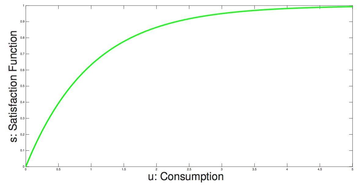
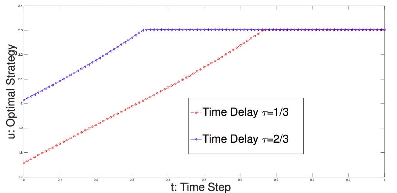
5 Decentralized Information and Partial Observation

Let $\mathcal{F}_{t}^{W}$ be the $\mathbb{P}$ -completed natural filtrations generated by $W$ up to $t$ . Set $\mathcal{F}^{W}:=\{\mathcal{F}_{t}^{W},\ 0\leq t\leq T\}$ and $\mathbb{F}:=\{{\mathcal{F}}_{t},\ 0\leq t\leq T\}$ , where $\mathcal{F}_{t}=\mathcal{F}_{t}^{W}\vee\sigma(x_{0})$ . An admissible control $u_{i}$ of agent $i$ is an $\mathcal{F}^{W_{i}}$ -adapted process with values in a non-empty, closed and bounded subset (not necessarily convex) $U_{i}$ of $\mathbb{R}^{d}$ and satisfies $E[\int_{0}^{T}|u_{i}(t)|^{2}dt]<\infty$ . Those are nonanticipative measurable functionals of the Brownian motions. Since each agent has a different information structure (decentralized information), let $\mathcal{U}_{i}$ be the set of admissible strategies of $i$ (with decentralized partial information) such that $\mathcal{G}_{i,t}\subset\mathcal{F}_{i,t},$ i.e., $\mathcal{U}_{i}:=\{u_{i}\in L^{2}_{\mathcal{G}_{i,T}}([0,T],\mathbb{R}^{d}),\ u_{i}(t,.)\in U_{i}\ \mathbb{P}-a.s\}.$ Given a strategy $u_{i}\in\mathcal{U}_{i}$ , and a (population) mean-field term $m$ generated by other agents we consider the signal-observation $x_{i}^{u_{i},m}$ which satisfies the following stochastic differential equation of mean-field type to which we associate a best-response to mean-field [158, 159, 132]:

\displaystyle\left\{\begin{array}[]{lll}\ \sup_{u_{i}\in\mathcal{U}_{i}}R(u_{i},m)\ \displaystyle{\mbox{ subject to }\ }\\ dx_{i}(t)=b(t,x_{i}(t),Ex_{i}(t),u_{i}(t),m(t))dt+\sigma(t,x_{i}(t),Ex_{i}(t),u_{i}(t),m(t))dW_{i,t},\\ x_{i}(0)\sim\mathcal{L}(X_{i,0}),\\ m(t)=\mbox{population mean-field },\end{array}\right.

b(t,x,y,u,m):\,\,[0,T]\times\mathbb{R}^{d}\times\mathbb{R}^{d}\times U_{i}\times\Lambda\longrightarrow\mathbb{R},

(46)

\sigma(t,x_{i},y_{i},u_{i},m):\,\,[0,T]\times\mathbb{R}\times\mathbb{R}\times U_{i}\times\Lambda\longrightarrow\mathbb{R}.

(47)

\begin{array}[]{l}\ R(u_{i},m)=g(x_{i}(T),Ex_{i}(T),m(T))+\int_{0}^{T}r(t,x_{i}(t),Ex_{i}(t),u_{i}(t),m(t))dt,\end{array}

$g$ is the terminal payoff and $r$ is the running payoff. Given $m,$ any $u^{*}_{i}\in{\cal U}_{i}$ which satisfies $R(u_{i}^{*}(\cdot),m)=\sup_{u_{i}(\cdot)\in{\cal U}_{i}}R(u_{i},m)$ is called a pure best-response strategy to $m,$ by agent $i.$ In addition to the other coefficient we assume that $\gamma$ satisfies H1. Under H1, the state dynamics admits a unique strong solution (see [161], Proposition 1.2.) Given $m,$ we apply the SMP for risk-neutral mean-field type control from ([162], Theorem 2.1) to the state dynamics $x$ to derive the first order adjoint equation. Under the assumption H1, there exists a unique $\mathbb{F}$ -adapted pair of processes $(p,q)$ , which solves the Backward SDE:

$\displaystyle p(t)$	$\displaystyle=$	$\displaystyle g_{x}(T)+E[g_{y}(T)]$	(48)
		$\displaystyle+\int_{t}^{T}\{H_{x}(s)+E[H_{y}(s)]\}ds$
		$\displaystyle-\int_{t}^{T}q(s)dW(s),$

such that $\mathbb{E}\left[\sup_{t\in[0,T]}\ |p(t)|^{2}+\int_{0}^{T}|q(t)|^{2}dt\right]<+\infty.$ However, these processes $(p,q)$ may not be adapted to decentralized information $\mathcal{G}_{i,t}.$ This is why their conditioning will appear in the maximum principle below. Again by ([162], Theorem 2.1), there exists a unique $\mathbb{F}$ -adapted pair of processes $(P,Q)$ , which solves the second order adjoint equation

	$\displaystyle P(t)=g_{xx}(T)$		(49)
	$\displaystyle+\int_{t}^{T}\{2b_{x}(s)P(s)+\sigma_{x}^{2}P(s)+2\sigma_{x}(s)Q(s)+H_{xx}(s)\}ds$
	$\displaystyle-\int_{t}^{T}Q(s)dW(s),$		(50)

such that $\mathbb{E}\left[\sup_{t\in[0,T]}\ |P(t)|^{2}+\int_{0}^{T}|Q(t)|^{2}dt\right]<+\infty.$ Note that in the multi-dimensional setting, the term $2b_{x}(s)P(s)+\sigma_{x}^{2}P(s)+2\sigma_{x}(s)Q(s)$ becomes $b^{\prime}_{x}P+Pb_{x}+\sigma^{\prime}_{x}P\sigma_{x}+\sigma^{\prime}_{x}Q+Q\sigma_{x}.$

Proposition 9.

Let H1 holds and $m$ be a given population mean-field profile. If $(x^{*}_{i},u^{*}_{i})$ is a best-response then, there are two pairs of $\mathbb{F}$ -adapted processes $(p,q)$ and $(P,Q)$ that satisfy (48) and (49) respectively, such that

\begin{array}[]{lll}i\in\mathcal{N}:\ \left[\delta H(t)+\frac{1}{2}\delta\sigma(t)^{\prime}P(t)\delta\sigma(t)\ |\ \mathcal{G}_{i,t}\right]\leq 0,\end{array}

(51)

for all $u_{i}\in\mathcal{U}_{i},$ almost every $t$ and $\mathbb{P}-$ almost surely, where,

\begin{array}[]{lll}\delta H(t):=H(t,x^{*}(t),u_{i},m(t),{p}(t),{q}(t))-H(t,x^{*}(t),u^{*}_{i}(t),m(t),{p}(t),{q}(t)),\end{array}

(52)

and $H_{k}(t):=b_{k}(t)p+\sigma_{k}(t)q+r_{k}(t),$ for $k\in\{x,y,xx\}.$

6 Limitations and Challenges

The examples above show that the continuum of agents assumption is rarely observed in engineering practice. The agents are not necessarily symmetric and a single agent may have a non-negligible effect on the mean field terms as illustrated in the HVAC application. Without having a broad set of facts on which to theorize, there is a certain danger of mean-field game models that are mathematically elegant, yet have little connection to actual behavior observed in engineering practice. At present, our empirical knowledge is inadequate to the main assumptions of the classical mean-field game theory. This is why a relaxed version is needed in order to better capture wide ranges of behaviors and constraints observed in engineering systems. MFTG relaxations include symmetry breaking, mixture between atomic and nonatomic agents, non-negligible effect on individual localized mean-field terms, and arbitrary number of decision-makers. In addition, behavioral and psychological factors should be incorporated for learning and information processes used by people-centric engineering systems. MFTG is still under development and is far from being a well-established tool for engineered systems. Until now, MFTG was not focused on behavioral and cognitively-plausible models of choices in humans, robots, machines, mobile devices and software-defined strategic interactions. Psychological and behavioral mean-field type game theories seem to explain behaviors that are better captured in experiments or in practice than classical game-theoretic equilibrium analysis. It allows to consider psychological aspects of the agent in addition to the traditional ”material” payoff modelling. The value depends upon choice consequences, mean-field states, mean-field actions and on beliefs about what will happen. The psychological MFTG framework can link cognition and emotion. It expresses emotions, guilt, empathy, altruism, spitefulness (maliciousness) of the agents. It also include belief-dependent and other-regarding preferences in the motivations. It needs to be investigated how much the psychology of the people matters in their behaviors in engineering MFTGs. The answer to this question is particularly crucial when analyzing the quality-of-experience of the users in terms of MOS (mean opinion score) values. A preliminary result from a recent experiment conducted in [111, 168] with 47 people carrying mobile devices with WiFi direct and D2D technology shows that the participation in forwarding the data of the users is correlated with their level of empathy towards their neighbors. This suggests the use of not only material payoffs but also non-material payoffs in order to better capture users behaviors. Another aspect of MFTGs is the complexity of the analysis (both equilibrium and non-equilibrium) when multiple agents (and multiple mean-field terms) are involved in the interaction [169, 71, 160, 132, 170].

7 Conclusion and Future Work

The article presented basic applications of mean-field-type game theory in engineering, covering key aspects such as de-congestion in intelligent transportation networks, control of virus spread over network, multi-level building evacuation, next generation wireless networks, incentive-based demand satisfaction in smart energy systems, synchronization and coordination of nodes, mobile crowdsourcing and cloud resource management. It appears from the wide ranges of applications and coverage that mean-field-type game theory is a promising tool for engineering problems. However, the framework is still under development and needs to be improved to capture realistic behavior observed in practice. Possible extensions of the work described in this article include the study of mean-field-type games for risk engineering, and an integrated mean-field-type game framework for smarter cities ranging from transportation to water distribution with ICT (Information Communication Technology), big data and human-in-the-loop among several other interesting directions.

Acknowledgments

This research work is supported by U.S. Air Force Office of Scientific Research under grant number FA9550-17- 1-0259. The authors would like to thank the Editor and the anonymous reviewers for interesting and constructive comments on the manuscript. The authors would like to thank the seminar participants at KTH Sweden for many extremely fruitful discussions and for their inputs on the first draft of the manuscript.

Conflict of Interest

The authors declare no conflict of interest in this paper.

References

[1] Wald A (1951) On Some Systems of Equations of Mathematical Economics. Econometrica 19: 368-403.
[2] von Neumann J, Morgenstern O (1953) Theory of Games and Economic Behavior, Princeton: Princeton University Press.
[3] Nash J., Non-Cooperative Games, Annals of Mathematics, Second Series, vol. 54, No. 2 (Sep., 1951), pp. 286-295.
[4] Wardrop JG(1952) Some theoretical aspects of road traffic research. P I Civil Eng 1: 325-378.
[5] Beckmann MJ, McGuire CB, Winsten CB(1956) Studies in the economics of transportation. Econ J 67:116-118.
[6] Knight FH (1924) Some fallacies in the interpretation of social cost. Q J Econ 38: 582 - 606.
[7] Dafermos SC, Sparrow FT (1969) The traffic assignment problem for a general network. J Res U.S. Natl Bur Stand 73B: 91-118.
[8] Larsson T, Patriksson M (1999) Side constrained traffic equilibrium models-analysis, computation and applications. Transp Res 33B: 233-264.
[9] Aashtiani HZ , Magnanti TL (1981) Equilibria on a congested transportation network. SIAM J Algebr Discrete Method 2: 213-226.
[10] Kohl JG (1841). Der verkehr und die ansiedelungen der menschen in ihrer abhangigkeit von der gestaltung der erdoberflache. Dresden/Leipzig: Arnold.
[11] Smith MJ (1979). The existence, uniqueness and stability of traffic equilibria. Transp Res,13B(4): 295 -304.
[12] Dafermos SC (1980). Traffic equilibrium and variational inequalities. Transp Sci;14(1): 42-54.
[13] Weibull J. (1995) Evolutionary Game Theory, Cambridge, MA: The M.I.T. Press, ISBN 0-262-73121-5
[14] Hofbauer J. and Sigmund K. (1988)Theory of Evolution and Dynamical Systems. Cambridge University Press, Cambridge.
[15] Hofbauer J. and Sigmund K (1998). Evolutionary Games and Population Dynamics. Cambridge University Press, Cambridge.
[16] Carlsson H. and van Damme E. (1993) Global Games and Equilibrium Selection, Econometrica, 61, 989-1018.
[17] Morris S. and Shin H. S. (1998), Unique Equilibrium in a Model of Self-Fulfilling Currency Attacks, American Economic Review, 88, 587-597.
[18] Dubey P. and Mas-Colell A. , and Shubik M. : Efficiency Properties of Strategic Market Games: An Axiomatic Approach, Journal of Economic Theory 22, 1980, pp. 339-362.
[19] Sandholm William H. (2010). Population Games and Evolutionary Dynamics. MIT Press, Cambridge.
[20] Samuelson L. (1997). Evolutionary Games and Equilibrium Selection. MIT Press, Cambridge.
[21] Friedman D. (1991) Evolutionary games in economics. Econometrica, 59: 637-666.
[22] Scarf H. (1962), An Analysis of Markets with a Large Number of Participants, In recent advances in Game Theory.
[23] Davis M. (1961): Symmetric solutions to symmetric games with a continuum of players, in recent advances in Game Theory.
[24] Debreu G. (1963), On a Theorem of Scarf, The Review of Economic Studies, vol. 30, No. 3 (Oct), pp. 177-180
[25] Shapley L. S. and Milnor J. W. (1978): Values of Large Games II: Oceanic Games, The RAND Corporation 1961, RM2649, also in Mathematics of Operations Research, 3:4 , pp. 290-307,
[26] Peleg B. (1963): Quota games with a continuum of players, Israel Journal of Mathematics, vol. 1, Issue 1, March 1963, pp. 48-53,
[27] Aumann R. J.(1964): Markets with a Continuum of Traders, Econometrica, vol. 32, pp. 39-50.
[28] Jovanovic B. (1982): Selection and the Evolution of Industry, Econometrica 50, pp. 649-670.
[29] Jovanovic B. and Rosenthal R. W.(1988). Anonymous sequential games, Journal of Mathematical Economics, vol. 17, pp. 77-87.
[30] Bergin J., Bernhardt D. (1992): Anonymous sequential games with aggregate uncertainty, Journal of Mathematical Economics, 21 (6) , pp. 543-562.
[31] Benamou J.-D. and Brenier Y. (2000): A computational fluid mechanics solution to the Monge-Kantorovich mass transfer problem. Numer. Math., 84(3), pp. 375-393.
[32] Benamou J. D. and Y. Brenier (2001). Mixed L2-Wasserstein optimal mapping between prescribed density functions. J. Optim. Theory Appl., 111(2), pp. 255-271.
[33] Lasry J.-M. and Lions P.-L.(2007) , Mean field games. Jpn. J. Math., 2(1), 2007, pp.229-260.
[34] Huang M.Y. , Malhame R.P. and Caines P.E. (2006). Large Population Stochastic Dynamic Games: Closed-Loop McKean-Vlasov Systems and the Nash Certainty Equivalence Principle, Special issue in honor of the 65th birthday of Tyrone Duncan, Communications in Information and Systems. Vol. 6, N. 3, pp 221-252.
[35] Zamir S., Maschler M., Solan E.(2013): Game Theory, Cambridge University Press; 1st Edition edition, ISBN-13: 978-1107005488
[36] A. Bensoussan, J. Frehse, S.C.P. Yam (2013): Mean field games and mean field type control theory, Springerbriefs in mathematics, Springer.
[37] Carmona R. and Delarue F. (2013), Probabilistic Analysis of Mean-Field Games, SIAM Journal on Control and Optimization, Vol. 51, No. 4, 2013, pp. 2705-2734.
[38] D. Gomes, S. Patrizi, and V. Voskanyan (2014). On the existence of classical solutions for stationary extended mean field games. Nonlinear Anal., 99:49-79.
[39] Diogo A. Gomes, Vardan K. Voskanyan: Extended Deterministic Mean-Field Games. SIAM J. Control and Optimization, 54(2): 1030-1055 (2016)
[40] Noha Almulla, Rita Ferreira, Diogo Gomes: Two Numerical Approaches to Stationary Mean-Field Games. Dynamic Games and Applications, 7(4): 657-682 (2017)
[41] Diogo A. Gomes, Vardan K. Voskanyan: Short-time existence of solutions for mean-field games with congestion. J. London Math. Society, 92(3): 778-799 (2015)
[42] Wilfrid Gangbo and Andrzej Swiech (2015), Existence of a solution to an equation arising from the theory of mean-field games, Journal of Differential Equations.
[43] J.-M. Lasry and P.-L. Lions (2006). Jeux à champ moyen. I. Le cas stationnaire. C. R. Math. Acad. Sci. Paris, 343(9),pp. 619-625.
[44] J.-M. Lasry and P.-L. Lions (2006). Jeux à champ moyen. II. Horizon fini et controle optimal. C. R. Math. Acad. Sci. Paris, 343(10), pp. 679-684.
[45] P.-L. Lions. College de France course on mean-field games. 2007-2011.
[46] P.-L. Lions. IMA, University of Minessota. Course on mean-field games. Video. http://www.ima.umn.edu/2012-2013/sw11.12-13.12/. 2012.
[47] Cardaliaguet, P., Delarue, F., Lasry J.-M., Lions P.-L. (2015). The master equation and the convergence problem in mean field games. Preprint
[48] A. Porretta (2015). Weak Solutions to Fokker-Planck Equations. Arch. Ration. Mech. Anal., 216(1):1-62.
[49] Bing-Chang Wang and Ji-Feng Zhang (2011). Distributed control of multiagent systems with random parameters and a major agent. Automatica.
[50] Bingchang Wang and Ji-Feng Zhang (2010). Mean field games for large population stochastic multi-agent systems with Markov jumps. Proceedings of the 29th Chinese Control Conference, , Beijing, China, July 29-31, pp. 4572-4577.
[51] M. Nourian, P. E. Caines, R. P. Malhame, and M. Huang (2012), Mean field LQG control in leader-follower stochastic multi-agent systems: Likelihood ratio based adaptation, IEEE Trans. Autom. Cont., vol. 57, no. 11, pp. 2801-2816.
[52] G. Y. Weintraub, L. Benkard, and B. Van Roy (2005). Oblivious equilibrium: A mean field approximation for large-scale dynamic games. Advances in Neural Information Processing Systems, 18, 2005.
[53] G. Y. Weintraub, C.L. Benkard, and B. Van Roy (2008). Markov perfect industry dynamics with many firms. Econometrica, November, 76(6):1375-1411.
[54] H. Tembine, J.-Y. Le Boudec, R. El Azouzi, E.Altman (2009): Mean field asymptotics of Markov Decision Evolutionary Games and teams. Gamenets: 140-150.
[55] D. Gomes, R. M. Velho, and M.-T. Wolfram (2014). Dual two-state mean- field games. Proceedings of IEEE CDC.
[56] D. Gomes, J. Mohr, and R. R. Souza. Discrete time, finite state space mean field games. Journal de Mathematiques Pures et Appliquees, 2010, 93(2): 308-328.
[57] D. Gomes, J. Mohr, and R. R. Souza (2013). Continuous time finite state mean-field games. Appl. Math. and Opt., 68(1):99-143.
[58] D.A. Gomes (2011). Continuous time finite state space mean field games - a variational approach. 49th Annual Allerton Conference on Communication, Control, and Computing, Allerton, pp 998- 1001.
[59] S. Adlakha, R. Johari, G. Weintraub, and A. Goldsmith (2008). Oblivious equilibrium for large-scale stochastic games with unbounded costs. Proceedings of the IEEE Conference on Decision and Control.
[60] J. Arabneydi and A. Mahajan (2014), Team optimal control of coupled subsystems with mean field sharing, in Proc. 53rd IEEE Conf. Decision and Control, Los Angeles, CA, Dec., pp. 1669-1674.
[61] M. Huang, P. E. Caines, and R. P. Malhame (2012), Social optima in mean field LQG control: centralized and decentralized strategies, IEEE Trans. Autom. Control, vol. 57, no. 7, pp. 1736 -1751.
[62] R. Elliott, X. Li, and Y.-H. Ni (2013), Discrete time mean-field stochastic linear-quadratic optimal control problems, Automatica, vol. 49, no. 11, pp. 3222-3233.
[63] D. Bauso, B. M. Dia, B. Djehiche, H. Tembine, R. Tempone (2014), Mean-Field Games for Marriage, PloS One, 9,5.
[64] A.-S. Sznitman. Topics in propagation of chaos. Ecole d’Ete de Probabilites de Saint-Flour XIXX1989, pages 165-251, 1991.
[65] D. Aldous: Exchangeability and related topics.In: Hennequin P(ed) Ecole d’Ete de Probabilites de Saint-Flour XIII-1983. Springer, Heidelberg. Lecture notes in mathematics, vol 1117, pp 1-198, (1985).
[66] H. Tembine, M. Huang: Mean field difference games: McKean-Vlasov dynamics. IEEE Conference on Decision and Control CDC-ECE, pp. 1006-1011, 2011
[67] Y. Achdou, Finite Difference Methods for Mean Field Games, Hamilton-Jacobi Equations: Approximations, Numerical Analysis 1 and Applications, Lecture Notes in Mathematics 2074, Springer-Verlag Berlin Heidelberg, 2013.
[68] Y. Achdou, F. Camilli, I. Capuzzo Dolcetta (2012), Mean field games: numerical methods for the planning problem. SIAM J. Control Optim. 50(1), 77-109.
[69] Y. Achdou, I. Capuzzo-Dolcetta (2010), Mean field games: numerical methods. SIAM J. Numer. Anal. 48(3), 1136-1162.
[70] Y. Achdou, V. Perez (2012), Iterative strategies for solving linearized discrete mean field games. Netw. Heterogeneous Media, 7(2), 197-217.
[71] H. Tembine: Nonasymptotic Mean-Field Games (2014). IEEE Transactions Cybernetics, 44(12): 2744-2756.
[72] A. Porretta (2013). On the planning problem for the mean-field games system. Dyn. Games Appl.
[73] K. Law, H. Tembine, R. Tempone (2016): Deterministic Mean-Field Ensemble Kalman Filtering, SIAM: SIAM Journal on Scientific Computing (SISC).
[74] S. Pequito, A. P. Aguiar, B. Sinopoli, and D. Gomes. Nonlinear estimation using mean field games. International Conference on NETwork Games, COntrol and Optimization, Netgcoop 2011, October 12-14, 2011, Paris, France.
[75] H. Yin, P. G. Mehta, S. P. Meyn and U. V. Shanbhag, Synchronization of Coupled Oscillators is a Game, IEEE Transactions on Automatic Control, 57:4, 920-935, April 2012.
[76] H. Yin, P. G. Mehta, S. P. Meyn and U. V. Shanbhag, Bifurcation Analysis of a Heterogeneous Mean-field Oscillator Game, In the Proceedings of the IEEE Conference on Decision and Control, Orlando, 3895-3900, Dec 2011.
[77] H. Yin, P. G. Mehta, S. P. Meyn and U. V. Shanbhag: On the Efficiency of Equilibria in Mean-field Oscillator Games,In the Proceedings of the American Control Conference, San Francisco, 53540-5359, June 2011.
[78] H. Yin, P. G. Mehta, S. P. Meyn and U. V. Shanbhag: Learning in Mean-field Oscillator Games, In the Proc. of the IEEE Conference on Decision and Control, Atlanta, 3125-3132, Dec 2010.
[79] L. Stella, F. Bagagiolo, D. Bauso, and G. Como, Opinion dynamics and stubbornness through mean-field games. 52nd IEEE Conference on Decision and Control December 10-13, 2013. Florence, Italy.
[80] A. Tcheukam Siwe, H. Tembine. Network Security as Public Good: A Mean-Field-Type Game Theory Approach, 13th International Multi-Conference on Systems, Signals & Devices, Conference on Systems, Automation & Control , Leipzig, Germany, 2016.
[81] Y. Wang, F. Richard Yu, H. Tang, and M. Huang: A Mean Field Game Theoretic Approach for Security Enhancements in Mobile Ad hoc Networks, IEEE Transactions on wireless communications, vol. 13, 3, March 2014.
[82] J. Moon and T. Basar. Discrete-time LQG mean field games with unreliable communication. Proc. 53rd IEEE Conference on Decision and Control (CDC’14, Dec 15-17, 2014; Los Angeles, CA), pp. 2697-2702.
[83] D. Bauso, H. Tembine, and T. Basar. Robust mean field games. J Dynamic Games and Applications, 2016
[84] A. Tcheukam and H. Tembine: Spatial Mean-Field Games for Combatting Corruption Propagation, 28th Chinese Control and Decision Conference (CCDC), Yinchuan, China, May 28 -30, 2016.
[85] M. Huang, P. E. Caines, and R. P. Malhame: Individual and mass behavior in large population stochastic wireless power control problems: centralized and Nash equilibrium solutions, in Proc. 42nd IEEE Conf. Decision Control,Maui, HI, Dec. 2003, pp. 98-103.
[86] F. Meriaux, V. Varma, and S. Lasaulce, Mean-field energy games in wireless networks, in Proc. Asilomar Conf. Signals, Syst., Comput, 2012
[87] F. Meriaux, S. Lasaulce, and H. Tembine. Stochastic differential games and energy-efficient power control. Dynamic Games and Applications, 2012.
[88] H. Tembine, P. Vilanova, M. Assaad, and M. Debbah, Mean field stochastic games for SINR-based medium access control, in Proc. Int Conf. Performance Evaluation Methodologies Tools, 2011.
[89] H.Tembine, E. Altman, R. El Azouzi, Y. Hayel: Evolutionary Games in Wireless Networks. IEEE Trans. Systems, Man, and Cybernetics, Part B 40(3): 634-646 (2010)
[90] H. Tembine , R. Tempone, P. Vilanova, Mean-field games for cognitive radio networks, in American Control Conference (ACC), 2012 , vol., no., pp.6388-6393, 27-29 June 2012
[91] H. Tembine, Energy-constrained Mean-Field Games in Wireless Networks, Strategic Behavior and the Environment: Vol. 4: No. 2, pp 187-21, 2014.
[92] R. Couillet, S. M. Perlaza, H. Tembine, and M. Debbah, A mean-field game analysis of electric vehicles in the smart grid, The 1st IEEE INFOCOM Workshop on Communications and Control for Sustainable Energy Systems: Green Networking and Smart Grids, Orlando, 2012.
[93] M. Kamgarpour, H. Tembine: A Bayesian mean-field game approach to supply demand analysis of the smart grid, First International Black Sea Conference on Communications and Networking (BlackSeaCom),pp 211-215, 2013.
[94] M. Manjrekar, V. Ramaswamy, S. Shakkottai (2014): A mean-field game approach to scheduling in cellular systems. INFOCOM 2014: 1554-1562
[95] A.F. Hanif, H. Tembine, M. Assaad, D. Zeghlache, Mean-Field Games for Resource Sharing in Cloud-Based Networks, IEEE/ACM Transactions on Networking, 24(1): 624-637 (2016).
[96] A. Farhan Hanif, H. Tembine, M. Assaad , D. Zeghlache, Cloud networking mean field games, IEEE 1st International Conference on Cloud Networking (CLOUDNET),pp: 46-50, 2012
[97] A. Khiyaita and M. Zbakh: Mean-field game among cloud computing end users, Security Days (JNS3), 2013 , pp 1 - 5
[98] Ghazzai H., Tembine H., Alouini M.S (2017): Mobile User Association for Heterogeneous Networks Using Optimal Transport Theory, In Proceedings of The Sixth International Conference on Communications and Networking, ComNet’2017, March 29th - April 1st
[99] K. Iyer, R. Johari, M. Sundararajan: Mean-Field Equilibria of Dynamic Auctions with Learning, EC’11, June 5-9, 2011, San Jose, California, USA
[100] K. Lyer, R. Johari, M. Sundararajan: Mean Field Equilibria of Dynamic Auctions with Learning. Management Science, 60(12), 2014, pp. 2949-2970
[101] D. Bauso, H. Tembine: Crowd-Averse Cyber-Physical Systems: The Paradigm of Robust Mean Field Games, IEEE Transactions on Automatic Control, 61(8): 2312-2317 (2016)
[102] J. Li, R. Bhattacharyya, S. Paul, S. Shakkottai, and V. Subramanian, Incentivizing Sharing in Realtime D2D Streaming Networks: A Mean Field Game Perspective, IEEE/ACM Transactions on Networking, 2016.
[103] A. Tcheukam Siwe and H. Tembine, Mean-Field-Type Games on Airline Networks and Airport Queues, 13th International Multi-Conference on Systems, Signals & Devices. Conference on Systems, Automation & Control. March 21 - 24, 2016 - Leipzig, Germany.
[104] M. Aziz, P. E. Caines: Computational investigations of decentralized cellular network optimization via mean field control. IEEE CDC 2014: 5560-5567
[105] J. Gao and H. Tembine: Distributed Mean-Field-Type Filter for Vehicle Tracking, 2017 American Control Conference, Seattle, WA, USA, May 24-26, 2017.
[106] J. Gao and H. Tembine: Correlative Mean-Field Filter for Sequential and Spatial Data Processing,17th IEEE International Conference on Smart Technologies, IEEE EUROCON 2017, 6 - 8 July 2017, Ohrid, Macedonia.
[107] P. Kachroo, S. Agarwal, S. Sastry (2016), Inverse Problem for Non-viscous Mean Field Control: Example From Traffic, IEEE Transactions on Automatic Control, DOI: 10.1109/TAC.2015.2511929.
[108] Tembine H. (2017), Mean-Field-Type Games, Workshop on Mean-Field Games, August 28-September 1, IPAM UCLA, Los Angeles, USA.
[109] J. Gao and H. Tembine: Distributed Mean-Field-Type Filters for Big Data Assimilation, IEEE International Conference on Data Science Systems (DSS 2016), Sydney, Australia Dec. 12-14, 2016
[110] J. Li, B. Xia, X. Geng, H. Ming, S. Shakkottai, V. Subramanian, and L. Xie, Mean Field Games in Nudge Systems for Societal Networks, ACM Sigmetrics 2015.
[111] G. Rossi, A. Tcheukam and H. Tembine (2016): How Much Does Users’ Psychology Matter in Engineering Mean-Field-Type Games, Workshop on Game Theory and Experimental Methods June 6-7, 2016
[112] Gao J. and Tembine H. (2017), Empathy and Berge equilibria in the Forwarding Dilemma in Relay-Enabled Networks, The International Conference on Wireless Networks and Mobile Communications (WINCOM’17)
[113] S. Grammatico, F. Parise, M. Colombino and J. Lygeros. Decentralized convergence to Nash equilibria in constrained mean field control, IEEE Transactions on Automatic Control, 2016.
[114] F. Parise, M. Colombino, S. Grammatico, and J. Lygeros, Mean-field constrained charging policy for large populations of plug-in electric vehicles, in Proc. of the IEEE Conference on Decision and Control, Los Angeles, California, USA, 2014, pp. 5101-5106.
[115] F. Parise, S. Grammatico, B. Gentile and J. Lygeros, Network Aggregative Games and Distributed Mean Field Control via Consensus Theory, Preprint 2016
[116] S. Grammatico, B. Gentile, F. Parise, J. Lygeros, A Mean Field control approach for demand side management of large populations of Thermostatically Controlled Loads, in Control Conference (ECC), 2015 European , vol., no., pp.3548-3553, 15-17 July 2015
[117] F. Bagagiolo and D. Bauso, Mean-field games and dynamic demand management in power grids, Dynamic Games and Applications, vol. 4, no. 2, pp. 155-176, 2014.
[118] H. Chen, Y. Li, R. Louie, and B. Vucetic, Autonomous demand side management based on energy consumption scheduling and instantaneous load billing: An aggregative game approach, IEEE Trans. on Smart Grid, vol. 5, no. 4, pp. 1744-1754, 2014.
[119] Z. Ma, D. Callaway, and I. Hiskens, Decentralized charging control of large populations of plug-in electric vehicles, IEEE Trans. on Control Systems Technology, vol. 21, no. 1, pp. 67-78, 2013.
[120] A. Kizilkale, S. Mannor, and P. Caines, Large scale real-time bidding in the smart grid: A mean field framework, Proc. of the IEEE Conf. on Decision and Control, pp. 3680-3687, 2012.
[121] R. Couillet , S.M. Perlaza , H. Tembine , M. Debbah, Electrical Vehicles in the Smart Grid: A Mean Field Game Analysis, IEEE Journal on Selected Areas in Communications, vol. 30, 6, pp: 1086-1096, 2012.
[122] H. Tembine, Mean-field-type optimization for demand-supply management under operational constraints in smart grid, pp 1-24, Energy Systems, 2015
[123] A. Tcheukam and H. Tembine: Mean-Field-Type Games for Distributed Power Networks in Presence of Prosumers, 28th Chinese Control and Decision Conference (CCDC), Yinchuan, China, May 28 -30, 2016
[124] M. Ye, G. Hu, Game Design and Analysis for Price based Demand Response: An Aggregate Game Approach, IEEE Transactions on Cybernetics, 2016
[125] D. Kun, P. Barooah, P.G. Mehta, Mean-field control for energy efficient buildings, in American Control Conference (ACC), 2012 , vol., no., pp.3044-3049, 27-29 June 2012
[126] A. C. Kizilkale, R. P. Malhame, Collective Target Tracking Mean Field Control for Electric Space Heaters, 22nd Mediterranean Conference on Control and Automation (MED) University of Palermo. June 16-19, 2014. Palermo, Italy 2014
[127] S. Klein (1976). A Design Procedure for Solar Heating Systems. Ph.D. thesis, Department of Chemical Engineering, University of Wisconsin-Madison.
[128] B. Gentile, S. Grammatico, J. Lygeros, Mean Field Modeling of Large-Scale Energy Systems, IFAC-PapersOnLine, vol. 48, Issue 1, 2015, pp. 918-919
[129] A. Kizilkale and R. Malhame, Mean field based control of power system dispersed energy storage devices for peak load relief, in IEEE Conference on Decision and Control (CDC), Dec. 2013, pp. 4971-4976.
[130] H. Tembine, Q. Zhu, T. Basar: Risk-Sensitive Mean-Field Games. IEEE Trans. Automat. Contr. 59(4): 835-850, 2014.
[131] J. Maynard Smith: Evolution and the Theory of Games. Cambridge University Press. ISBN 0-521-28884-3, 1982
[132] H. Tembine, Risk-sensitive mean-field-type games with p-norm drifts, Automatica, vol. 59, September 2015, pp. 224-237, ISSN 0005-1098.
[133] M. Fornasier and F. Solombrino. Mean-field optimal control. ESAIM Control Optim. Calc. Var., 20(4):1123-1152, 2014.
[134] D. Andersson and B. Djehiche, A maximum principle for SDEs of mean-field type. Appl. Math. Optim. 63(3), 2010, 341-356.
[135] A. K. Cisse, H. Tembine: Cooperative Mean-Field Type Games, 19th World Congress The International Federation of Automatic Control, Cape Town, South Africa. August 24-29, 2014
[136] X. Luo, H. Tembine (2016): Evolutionary coalitional games for random access control, Annals of Operations Research, to appear, 2016, pp 1-34.
[137] A.Tcheukam Siwe, H. Tembine. On the distributed mean-variance paradigm, 13th International Multi-Conference on Systems, Signals & Devices, Conference on Systems, Automation & Control, Leipzig, Germany, 2016.
[138] H. Tembine, Population games with networking applications, PhD Thesis, Universite d’Avignon, 2009.
[139] P. Taylor, L. Jonker (1978), Evolutionarily Stable Strategies and Game Dynamics, Mathematical Biosciences, 40, 145-156.
[140] B. Djehiche, A. Tcheukam and H. Tembine: A Mean-Field Game of Evacuation in a Multi-Level Building, Special Session 118: Mean field games and applications, The 11th AIMS Conference on Dynamical Systems, Differential Equations and Applications, July 1 - 5, 2016, Orlando, Florida, USA
[141] B. Djehiche, A. Tcheukam and H. Tembine: Evacuation of Multi-Level Building: Design, Control and Strategic Flow, 35th Chinese Control Conference (CCC2016), July 26-28 Southwest China, Chengdu.
[142] B. Djehiche, A. Tcheukam and H. Tembine: A Mean-Field Game of Evacuation in a Multi-Level Building, 17th International Symposium on Dynamic Games and Applications, Urbino, Italy, July 12-15, 2016
[143] B. Djehiche, A. Tcheukam and H. Tembine: A Mean-Field Game of Evacuation in a Multi-Level Building, IEEE Transactions on Automatic Control, DOI: 10.1109/TAC.2017.2679487, Volume: 62, Issue: 10, Oct. 2017, pp. 5154 - 5169
[144] D. Duives, W. Daamen, S. Hoogendoorn: State-of-the-art crowd motion simulation models, Transportation Research Part C: Emerging. Technologies, 37 , 2013, pp. 193-209.
[145] D. Helbing, A. Johansson, Pedestrian, crowd and evacuation dynamics, Encyclopedia of complexity and System Science, 16 , 2010, pp. 6476-6495.
[146] S. P. Hoogendoorn, F. van Wageningen-Kessels, W. Daamen, D. C. Duives, M. Sarvi: Continuum Theory for Pedestrian Traffic Flow: Local Route Choice Modelling and its Implications, In Transportation Research Procedia,vol. 7, 2015, pp 381-397, 21st International Symposium on Transportation and Traffic Theory, Kobe, Japan, 5-7 August, 2015.
[147] P. Degond, J. Hua Self-organized hydrodynamics with congestion and path formation in crowds, Journal of Computational Physics, 2013.
[148] R. Hughes: A continuum theory for the flow of pedestrians, Transportation Research Part B: Methodological, 36, 2002, pp. 507-535.
[149] C. Villani, Optimal Transport: Old and New, Springer Book, Grundlehren der mathematischen Wissenschaften, vol. 338, 2009, ISBN: 978-3-540-71049-3.
[150] N. Bellomo and C. Dogbe: On the Modelling of Traffic and Crowds, A Survey of Models, Speculations, and Perspectives. SIAM Review, Vol 53, No. 3, pp. 409-463, 2011.
[151] A. Lachapelle, M.-T. Wolfram. On a mean field game approach modeling congestion and aversion in pedestrian crowds. Transportation Research Part B: Methodological vol. 45, Issue 10, December 2011, pp. 1572-1589
[152] M. Burger, M. Di Francesco, P.A. Markowich, M.T. Wolfram, Mean field games with nonlinear mobilities in pedestrian dynamics, DCDS 19(5), 1311–1333, 2014
[153] M. Burger, M. Di Francesco, P. Markowich, M.T. Wolfram, On a Mean Field Game Optimal Control Approach Modeling Fast Exit Scenarios in Human Crowds, 52nd IEEE Conference on Decision and Control, Firence, Italy, 2013.
[154] Gomes D. A. and Patrizi S. . Obstacle mean-field game problem. Interfaces Free Bound., 17(1):55-68, 2015.
[155] Tembine H., Vilanova P., Debbah M.: Noisy Mean Field Game Model for Malware Propagation in Opportunistic Networks, vol. 75 of the series Lecture Notes of the Institute for Computer Sciences, Social Informatics and Telecommunications Engineering pp 459-474,
[156] Kuramoto Y., Self-entrainment of a population of coupled non-linear oscillators, In International Symposium on Mathematical Problems in Theoretical Physics, Lecture Notes in Physics,, Vol. 39, pp. 420-422, Springer, New York, 1975.
[157] Zhihao Xu, Magnus Egerstedt, Greg Droge and Klaus Schilling: Balanced Deployment of Multiple Robots Using a Modified Kuramoto Model, American Control Conference (ACC) Washington, DC, USA, June 17-19, 2013
[158] Djehiche B., Tembine H., Tempone R. (2015): A Stochastic Maximum Principle for Risk-Sensitive Mean-Field Type Control. IEEE Trans. Automat. Contr. 60(10): 2640-2649.
[159] Djehiche B. ,Tembine H. (2016): Risk-Sensitive Mean-Field Type Control Under Partial Observation, Chapter in Stochastics of Environmental and Financial Economics, vol. 138 of the series Springer Proceedings in Mathematics & Statistics.
[160] H. Tembine, Uncertainty Quantification in Mean-field-type Teams and Games, IEEE CDC, 2015.
[161] B. Jourdain, S. Meleard, W. Woyczynski, Nonlinear SDEs driven by Lévy processes and related PDEs. Alea 4, 2008, pp. 1-29.
[162] R. Buckdahn , B. Djehiche and J., Li: A general stochastic maximum principle for SDEs of mean-field type. Applied Math. and Optimization, 64(2), 2011, pp. 197-216.
[163] F. Cucker and S. Smale (2007) , Emergent behavior in flocks , IEEE Trans. Autom. Control , vol. 52 , no. 5 , pp.852-862, 2007
[164] F. R. Millikan (2012), Joseph Henry: Father of Weather Service? Joseph Henry Papers Project, Smithsonian Institution.
[165] Henson Pamela M. (2006): Spencer F. Baird’s Vision for a National Museum.
[166] Krause A. , Horvitz E., Kansal A., Zhao F. (2008): Toward Community Sensing, pp. 481 - 492, 22-24 April , Print ISBN: 978-0-7695-3157-1,St. Louis, MO.
[167] Schwartz G. , Tembine H., Amin S., Sastry S. (2014), Demand Response Scheme Based on Lottery-Like Rebates, Proceedings of the 19th IFAC World Congress
[168] Tembine H. (2015), Learning and Game Theory Lab: the game of life, International innovation, September 2015, pp. 49-51, http://www.internationalinnovation.com/the-game-of-life/
[169] H. Tembine: Large-scale games in large-scale systems, Proceedings of the 5th International Conference on Performance Evaluation Methodologies and Tools, 2011, pp 9-17
[170] D. Bauso, H. Tembine, T. Başar, Opinion dynamics in Social Networks through mean-field games, SIAM Journal on Control and Optimization, Society for Industrial and Applied Mathematics, Vol. 54, No. 6, pp. 3225-3257, 2016
[171] Tembine H. (2017): Reverse Ishikawa-Nesterov Learning Scheme for Fractional Mean-Field Games, 20th World Congress of the International Federation of Automatic Control (IFAC) , Toulouse, France, 9-14 July 2017
[172] Tembine H. (2017), Swarm Learning in Discrete Time Mean-Field-Type Games, Conference on Systems, Automation & Control, International Multi-Conference on Systems, Signals & Devices
[173] Tembine H. (2017), The Price of Simplicity of Mean-Field-Type Optimization is Unbounded, Conference on Communication, Signal Processing & Information Technology, International Multi-Conference on Systems, Signals & Devices.
[174] Tembine H. (2017), Quantile-based Mean-Field Games, Conference on Power Systems & Smart Energies, International Multi-Conference on Systems, Signals & Devices.
[175] H. Tembine (2017): Payoff Measurement Noise in Risk-Sensitive Mean-Field-Type Games, 29th Chinese Control and Decision Conference, May 28-30, Chongqing, China.
[176] Duncan TE, Tembine H (2017) Linear-quadratic mean-field-type games: A direct method, Preprint.
[177] Duncan TE, Tembine H (2017) Linear-quadratic mean-field-type games with common noise: A direct method, Preprint.
[178] Duncan TE, Tembine H (2017) Other-regarding payoffs in linear-quadratic mean-field-type games with common noise: A direct method, Preprint.
[179] H.Tembine, B. Djehiche, P. Yam, A. Bensoussan: Mean-Field-Type Games with Jumps and Switching Regimes, Preprint 2017
[180] Dubey P. (1986). Inefficiency of Nash equilibria. Math. Operat. Res., 11(1):1-8.
[181] Koutsoupias E, Papadimitriou C (1999): Worst-case Equilibria. Proceeding STACS’99 Proceedings of the 16th annual conference on Theoretical aspects of computer science pp 404-413
[182] Koutsoupias E, Papadimitriou C (2009): Worst-case Equilibria. Computer Science Review. 3 (2): 65-69.
[183] Tanimoto, J.: Fundamentals of Evolutionary Game Theory and its Applications, Springer, 2015.10; ISBN: 978-4-431-54961-1