Gamma-ray signals from dark matter annihilation via charged mediators
Abstract
We consider a simplified model in which Majorana fermion dark matter annihilates to charged fermions through the exchange of charged mediators. We consider the gamma-ray signals arising from the processes , , and in the most general case, including nontrivial fermion mass and nontrivial left-right mixing and the -violating phase for the charged mediators. In particular, we find the most general spectrum for internal bremsstrahlung, which interpolates between the regimes dominated by virtual internal bremsstrahlung and by final state radiation. We also examine the variation in the ratio and the helicity asymmetry in the process, each as a function of the mixing angle and -violating phase. As an application, we apply these results to searches for a class of minimal supersymmetric Standard Model.
Keywords:
TBDpacs
14.80.LyI Introduction
The nature of dark matter has long been a puzzle in modern physics. It is suspected to be a very long-lived massive particle, while currently no evidence shows that it carries electrical or color charge. Such a particle cannot be described by the Standard Model (SM) of particle physics. The most recent measurement of the dark matter abundance from the Planck satellite is [1]. If we assume that dark matter consists of weakly interacting massive particles (WIMPs) with mass ranging from to , the standard thermal freeze-out mechanism yields the qualitatively correct relic density [2, 3, 4, 5, 6, 7]. As a result, the WIMP hypothesis is very attractive, but by no means required. Searches for the interaction of dark matter with SM matter are ongoing, utilizing a variety of strategies, including direct, indirect, and collider-based searches.
The main purpose of this paper is to analyze the associated gamma-ray signals that may be observable in indirect dark matter searches if Majorana fermion dark matter couples to light SM fermions via charged mediators. Such couplings arise in a variety of dark matter scenarios, including the minimal supersymmetric Standard Model (MSSM), in which the lightest supersymmetric particle (LSP) is a dark matter candidate, and its bino component can couple to SM fermions through the - or -channel exchange of sfermions. Moreover, the gamma-ray signals from dark matter annihilation in this scenario are often crucial to observational strategies, because gamma-ray signals are relatively clean, and because the direct annihilation process is often suppressed.
The processes which we will consider are , , and . All of these processes have been considered in the past [8, 9, 10, 11], but either for special cases or different purposes. Our goal here will be to consider the most general spectra that can arise for these processes in a simplified model in which a Majorana fermion dark matter particle couples to a Dirac fermion (which may or may not be a SM fermion) through the exchange of two charged scalars, with an arbitrary left-right mixing angle and -violating phase. Examples of this simplified model exist within the parameter space of the MSSM, including the “Incredible Bulk” models described in Ref. [12], but the applicability is much broader.
The main new features which we will find are:
- •
The complete spectrum for the process as a function of mixing angle, which interpolates between the hard regime, dominated by virtual internal bremsstrahlung, and the soft regime, dominated by soft and collinear final state radiation
- •
The ratio of the cross sections for and as a function of mixing angle and -violating phase
- •
The difference in rates for the production of left-circularly and right-circularly polarized photons via the process
This article is organized as follows: In Sec. (II), we briefly describe the effective model and the parameter space in which we are interested. We then discuss the general features of the relevant gamma-ray signals in Sec. (III). In Sec. (IV), we describe the monochromatic line signals, and their observational impact. In Sec. (V), we similarly describe the general internal bremsstrahlung gamma-ray signature. Finally our chief results are summarized in Sec. (VI).
II Model and Its General Features
We consider a simplified model in which the dark matter candidate is a SM gauge singlet Majorana fermion and the only relevant interaction is
| (1) |
where are the chiral projectors. Here, is a fermion charged11 1 For simplicity, we assume the charge be . under , and are the charged scalar mediators. We also assume that the dark matter is absolutely stable because it is the lightest particle charged under an unbroken hidden symmetry, and the are also charged under the same symmetry. But the fermion is uncharged under the symmetry that stabilizes the dark matter.
The mass eigenstates and chiral eigenstates of the scalar mediators are related by a mixing angle ,
| (2) |
We denote the two mass eigenvalues as and in the following. To ensure that the dark matter is stable, we assume . However, can be either larger or smaller than .
We also allow a nonzero -violating phase, , such that the coupling constants may be expressed as
| (3) |
We are thus left with seven free parameters for this simplified model:
In the MSSM framework, if is a purely binolike LSP and there is a single generation of light sfermions, then we have and , where is the gauge coupling and are the scalar hypercharges. This scenario has been considered recently in Ref. [12, 13, 14]. We also briefly consider the possibility of a new heavy fermion, in which case there is an additional parameter necessary to specify its mass, .
Note that only the relative phase between and is physically significant, since any overall phase can be removed by a vectorlike phase rotation of . Similarly, although the most general matrix relating the scalar mass and chiral eigenstates contains three complex phases, they can be absorbed by a phase rotation of the chiral eigenstates, , and the mass eigenstates, . Having chosen to make the mixing matrix real, one cannot then use a chiral rotation of the to rotate away the phase . However, if , the requirement that the mixing matrix be real only fixes two phases; in this case, the phase can then be absorbed into a chiral rotation of the . Similarly, if , then the phase can be removed by a chiral rotation of . As a result, -violating effects must scale as .
II.1 General features
If the cross section for the process is not suppressed, it will dominate over processes such as and , which will be suppressed by factors of at least and , respectively. In this case, prompt gamma-ray signals are sometimes considered to be less promising from an observational standpoint, because models that would produce prompt gamma-ray signals large enough to be observed with current or near future experiments can already be probed by searches for cosmic rays produced by the process . However, current exclusion limits based on searches for positrons or antiprotons are subject to large systematic uncertainties related to assumptions about the astrophysical background and propagation of charged particles in our Galaxy; if these assumptions are weakened, then the exclusion limits from cosmic-ray searches can be similarly weakened, permitting even the suppressed , , and signals to be relevant. The Feynman diagrams for the two-body annihilation and internal bremsstrahlung are shown in Fig. 1, while those for the one-loop process are shown later in Fig. 11 of Appendix A, where a detailed discussion on this process is presented.
But there are two scenarios in which the annihilation cross section is suppressed:
- •
If , then is not kinematically allowed.
- •
If there is minimal flavor violation (MFV), then the cross section for the process is suppressed by a factor .
In the case where , the processes are forbidden, allowing the processes and to be the most important (other processes, such as may have similar cross sections but are likely to be less observationally important compared to a clean gamma-ray signal). This scenario is relevant in the case where dark matter couples to a new, heavy charged fermion.
In the case where , the cross section for the process must scale with the remaining parameters, which breaks flavor symmetry. The reason is that, because the dark matter is Majorana and the initial state wave function must be antisymmetric, the -wave initial state must have . The final state and must then have the same helicity, implying that the and arise from different Weyl spinors. The final state is thus not invariant under chiral flavor symmetries and must vanish in the limit in the case of MFV .
In the simplified model that we consider here, the only deviation from MFV arises from the presence of nontrivial mixing of the scalar chiral eigenstates. This requires both a nontrivial left-right mixing angle and nondegeneracy of the mass eigenstates (if the mass eigenstates are degenerate, then a redefinition of the eigenstates is sufficient to absorb the mixing angle). In the massless fermion limit, left-right mixing gives an -wave two-body annihilation amplitude of
| (4) |
where we denote the initial state dark matter momenta as and the final state fermion momenta as and ; and are spinor wave functions, following the definition of Ref. [15]. This amplitude leads to the cross section
| (5) |
In the scenario, the charged fermion must necessarily be a SM fermion.
II.2 Constraints from colliders and lepton dipole moments
The discovery of the SM-like Higgs boson [16, *ATLAShiggs] at the LHC is a triumph of the SM. Meanwhile, null searches for supersymmetric particles imply a lower limit of for light degenerate first and second generation squarks [18]. Constraints on squark masses in the simplest predictive supersymmetric model, the constrained MSSM (CMSSM), are even more stringent, and exclude squarks below for certain benchmark models [18, *CMSsquark]. If we relax some unification constraints imposed in the CMSSM at the grand unified theory scale, then it has been shown that the MSSM-9 model [20, *cabrera2] can contain a Higgsino LSP or a wino LSP, which are viable thermal dark matter candidates satisfying the relic density.
On the other hand, the current limit on the mass of any slepton is much weaker. We still have the possibility that heavy squarks provide the necessary loop corrections to the mass of the SM-like Higgs while light sleptons provide the main dark matter annihilation channel. Large Electron-Positron Collider (LEP) experiments only put a lower limit at [22, *L3, *DELPHI, *OPAL], while the LHC run has excluded left-handed sleptons below and right-handed sleptons below , assuming a massless bino LSP [26, *CMSslepton]. For a massive bino LSP with mass , a new allowed region opens up for sleptons lighter than approximately [26, *CMSslepton]. The LHC run has the potential to push the upper exclusion limit to as high as (for a Higgsino LSP) but cannot move the lower exclusion limit [28].
Although these constraints are phrased as bounds on scalar superpartners, the lesson is more general: LHC constraints place tight bounds on colored scalars but weaker bounds on QCD-neutral scalars. Since the must necessarily be QCD charged if is a quark, we will assume that, if is a SM fermion, it is a lepton.
A new correction to the electric and magnetic dipole moments of the SM fermions arises from diagrams with and the new charged mediator running in the loop; if is a SM fermion, then the can be constrained by bounds on fermion dipole moments [29, 12] (in the absence of fine-tuned cancellations against other contributions to the dipole moments from independent new physics). In the case where is a SM charged lepton, the constraints can be summarized as follows:
- •
The cross section is constrained to be , absent fine-tuning.
- •
The cross section is constrained to be , absent fine-tuning, unless violation is close to maximal (). This constraint arises because the muon magnetic dipole moment is much more tightly constrained than its electric dipole moment. For near-maximal violation, the annihilation cross section must be less than , absent fine-tuning.
- •
The cross section can easily be , or larger. For our purposes, it is unconstrained by dipole moment bounds.
We close this section by noting that although our model fits within the MSSM, it can also serve as a simplified model for other scenarios in which a gauge singlet Majorana dark matter couples only to a fermion and two scalar particles.
III Gamma-Ray Signals
In the current era, it is believed that there are potentially observable excesses of dark matter particles near our Galactic center and in nearby dwarf galaxies. The ongoing annihilations of these dark matter particles may result in observable cosmic-ray signals, such as in the cosmic gamma-ray spectrum and/or in the cosmic-ray positron and/or antiproton fraction. Typically, various reactions involving the final state lepton pairs result in an almost featureless secondary photon spectrum. In the simplified model we consider, however, a distinctive feature may be contained in the internal bremsstrahlung (IB) spectrum and the associated line signals.
The search for line signals of dark matter annihilation has been one of the primary goals of various ground-based and satellite-based experiments. In general, the ground-based atmospheric Cherenkov telescopes [30, *CTA] are most effective for dark matter that is somewhat heavier than 100 GeV. For example, with 500 h of observing time, Cherenkov Telescope Array (CTA) will be sensitive to cross sections for dark matter with mass of annihilating to in the Galactic center region [32]. Due to its much lower energy threshold, the Fermi Gamma-Ray Space Telescope is better suited to study dark matter masses in the range to a few hundred GeV, which is the range we are interested in here. For GeV, the Fermi Large Area Telescope (LAT) has set a limit on the thermally averaged annihilation cross section to of with the C.L. containment spanning approximately one order of magnitude using the PASS 8 analysis of yr of data [33]. However, this limit, as well as any projected sensitivities, is sensitive to the dark matter profile of the Milky Way halo and may move up or down by about one order of magnitude for different profiles. We hope that the sensitivity to will be improved with additional data and/or new technology. Future satellite-based experiments GAMMA-400 [34] and HERD [35] are expected to reach for . In addition, each of these experiments is expected to have energy resolution of , which is much better than Fermi-LAT’s ( at ), making it possible to distinguish between a sharply peaked IB spectrum and a true line signal.
Here, we present our results for the bremsstrahlung and other prompt photon emissions arising from dark matter annihilation to fermions and monochromatic emissions from annihilation to and . By prompt emission, we mean the photons produced directly at the dark matter annihilation, including, for example, the hadronic decay of the final state . On the other hand, the photon emission due to inverse Compton scattering and bremsstrahlung in the Galactic electromagnetic fields (so-called secondary emission), which depends on modeling of the dark matter distribution and cosmic-ray propagation, is not included.
The photon spectrum is defined as the photon number per annihilation per energy bin, and can be broken into a continuum spectrum and a contribution from monochromatic photons:
| (6) |
In our case, the continuum spectrum comes mainly from IB and other prompt emission from the final state particles,
| (7) |
where is the number of photons produced in a single annihilation process and the sum over includes all higher order prompt emissions, and is the IB cross section, which will be described in Sec. V. Note that the spectrum is normalized by , the total annihilation cross section. When there is no chiral mixing, its dominant component is the total IB cross section. As discussed below, the line spectrum consists of the and peaks,
| (8) |
where as given in Eq. (9). These definitions follow Ref. [36].
IV Monochromatic Gamma-Ray Line Signals
Monochromatic lines in the gamma-ray spectrum arise due to the one-loop annihilation process , where or . The photon(s) in the final state has (have) energy
| (9) |
where is the mass of the particle . energy resolution is sufficient to differentiate and lines for . In the Galactic center, the relative velocity between dark matter particles is , so the -wave component of the dark matter annihilation cross section is suppressed.
The -wave () component must arise from a spin-singlet initial state (), since the dark matter particles are Majorana fermions and must be in a totally antisymmetric initial state. This state thus necessarily has vanishing total angular momentum (), implying that the final state particles must have the same helicity. As a result, only the and cross sections can develop nonvanishing -wave components, while the leading cross section must be -wave suppressed and is thus too small to be observed.
To ensure the accuracy of the results presented here, we perform a scan over the parameter space, conducted as follows. We first generate the analytic amplitudes for both and using FeynArts [37], including left-right scalar mixing and a -violating phase (the amplitude is presented in Appendix A). The numerical calculation is performed using FormCalc [38]. The package LoopTools is internally invoked by FormCalc to calculate the loop integrals involved in the amplitudes. However, since our initial state particles are at rest, we have . It is well known that if two external momenta are collinear, the Gram matrix becomes singular and the tensor loop integrals fail to be linearly independent. For analytic calculation, this is a virtue and essentially the reason why all the four-point loop integrals that appear in the amplitude can be reduced to three-point scalar loop integrals (see Appendix A)22 2 For a comprehensive review on the calculation techniques of general tensor loop integrals, see Ref. [39].. Numerically, FormCalc breaks down for collinear external momenta, since LoopTools uses precisely the Gram matrix to derive higher-point and higher-rank integrals.
To circumvent this issue and arrive at a reliable result, we introduce a small relative velocity, so that the results of LoopTools remain stable. For example, we use a center-of-mass energy of for in our numerical calculations. We have checked that the numerical error in the cross section is for annihilations to both and (with scalar mixing), independent of the model parameters. For -wave dominant cross sections, we perform a linear fit with respect to to find the coefficients and in the expansion . We have also checked that the error is in this scenario.
Analytic MSSM calculations of the annihilation cross section to and have been presented in Ref. [8, 9, 10] in the limit of no violation, and those expressions are consistent with the ones presented here. However, if , then the amplitude of the photon helicity state will be different from that of the state, unlike the case. As we argued previously, the difference in the scattering amplitude is chirally suppressed by the fermion mass ,
| (10) |
a term which does not appear previously in the literature. We defer the full analytic expressions for the cross section, including chiral mixing and violation, to Appendix A.
In order for violation to yield differing cross sections for the and final photon states, it is necessary for . If , then the -violating part of the amplitude is purely imaginary (as a result of the optical theorem), and conjugation of the matrix element is equivalent to complex conjugation. But if , then the intermediate states of the one-loop diagram can go on shell, providing an imaginary component to the -conserving matrix element, which is necessary for a nontrivial asymmetry. On the other hand, if , then the only final states that are kinematically allowed are and . In this kinematic regime, if the couplings are large, these final states will be most easily observable.
We would like to make a few general comments regarding the sensitivity of the dark matter annihilation cross sections into and to scalar chiral mixing and violation. First, both cross sections decrease as the scalar masses increase. Thus to make a sizable line signal, we need to have at least one scalar mass not too much heavier than the dark matter. If they are very degenerate, of course, coannihilations, not considered here, would also play a role in determining the relic density. Second, the ratio increases as the difference between the two scalar masses increases. As a very crude estimate, this ratio is approximately , which works well at no mixing. However, by varying the mixing angle and -violating phase, we can make it as large as within the MSSM.
In the following discussion, we will focus on several benchmark models, displayed in Table 1. Models , , and are consistent with a supersymmetric implementation of the Lagrangian in Eq. (1), while models and are explicitly nonsupersymmetric due to the couplings and, in the case of model , an additional heavy fermion. Note that, for all of these benchmark points, the new charged particles are fully consistent with constraints from the LHC and LEP.
Benchmark presents an interesting case, as it contains a new charged fermion with . Such a particle is within the energy reach of the LHC, and one must worry if such a particle would already be excluded by current data. But LHC sensitivity to new charged particles depends greatly on the particle decay chains; it is easy to choose a decay scenario for which would escape current LHC limits. For example, if the new fermion decayed to a SM charged lepton and a new invisible scalar, then this charged fermion would escape detection for the same reason that light sfermions do in the compressed spectrum scenario. The new invisible scalar need not contribute to dark matter, or even be long lived, provided its lifetime was long enough to decay outside the detector. We will not focus further on this particular decay scenario, which we describe only to demonstrate that benchmark can be completely consistent with LHC constraints. For models where is even larger, LHC constraints may be more easily satisfied, without qualitatively changing the analytic results we obtain.
| Channel | Marker | |||||
| Star | ||||||
| Circle | ||||||
| Cross | ||||||
| Square | ||||||
| Diamond | ||||||
| , GeV | 2 | 2 | Triangle |
In the following subsections, we examine the line signal strengths in the context of different SUSY and non-SUSY models.
IV.1 SUSY case
We first consider the SUSY case, as in Ref. [12], where and are SM leptons and MSSM sleptons, therefore denoted as and in this subsection. In Fig. 2, we display the cross sections (left) and (right) as functions of for , , and . Since is only mildly sensitive to the -violating phase, , we show the cross section as a function of for in the inset of the right panel. Turning first to the left panel, we see an increase of by a factor of as ranges from zero to at (and as much as a factor of over the full range of shown). For the channel, displayed in Fig. 2, the dependence on is significant (in contrast to the channel): At , varies by a factor of 2 as ranges from zero to . Turning to the right panel, we see that there is an increase in by about a factor of for relative to . This arises from the fact that : for (), the lighter scalar mass eigenstate consists entirely of the right-handed (left-handed) component, the contribution to the cross section of which is proportional to (). This enhancement is possible only when the two-body annihilation cross section is suppressed ( for odd), and thus the relic abundance of binos is too large. If another mechanism, such as coannihilation, helped to lower the relic abundance, or if dark matter were nonthermal, it may be possible for the line signal to be much larger than that suggested by the benchmark points. As we see in the right panel of Fig. 2, the dependence of on the -violating phase is not as significant as it is for annihilation to , even for the channel.
In Fig. 3, we display a contour plot of with respect to the chiral mixing, , and -violating phase, . The regions of parameter space in which the dark matter is a thermal relic are shaded blue, and, for the channel, the regions compatible with the measurement of the muon anomalous magnetic moment are shaded red/magenta (for the channel, the dipole moment measurements do not constrain the parameter space). Benchmarks A, B, and C are also marked.
Unfortunately for the SUSY case, these monochromatic photon signals lie well below the current experimental sensitivity. Nonetheless, it is worth considering the possibility of an eventual detection. As discussed in Sec. IV, once a statistical excess of these line signals is observed, and if the dark matter mass lies in the range (for Fermi-LAT) or (for GAMMA-400 or HERD), the ratio of the dark matter annihilation cross section into and will be of significant interest for determining the nature of the dark matter particle and the theory of physics beyond the SM in which it resides. Indeed, this ratio does not suffer from astrophysical uncertainties in the dark matter distribution in our Galaxy [8]. In Ref. [40], a wide range of MSSM parameter space is examined, and an attempt is made to use the ratio of to distinguish among coannihilation, funnel, and focus point scenarios in mSUGRA, as well as within more general MSSM scenarios.
Following the same line of analysis, we plot the annihilation cross section to (left) and the ratio (right) as functions of the slepton masses in Fig. 4 for the (top) and (middle and bottom) channels for and . In the top panels, we display the channel with and in the middle and lower panels, we display the tau channel with and , respectively. In the left panels, we display the cross sections in units of , while in the right panels we show the ratio . The parameter space that accommodates thermal relic dark matter lies between the thick dashed contours that cut diagonally across each plane. As expected, decreases as the slepton masses increase. Similarly, the ratio increases as the difference between and increases. is larger than 17.0 for in the channel. Although not presented in Fig. 4, this approximately holds true for the channel as well. In the case of , is greater than for the channel and greater than for the channel. By contrast, in the coannihilation region in minimal supergravity (mSUGRA), ranges from (see Fig. 5 in Ref. [40]). It is therefore possible that if both the and lines are observable, the ratio of the signal strengths could be used to distinguish between, for example, the coannihilation region and a model similar to the Incredible Bulk. Though these scenarios could, in principle, also be distinguished by the cosmic-ray signal arising from , such a signal would be subject to astrophysical uncertainties and would therefore leave much room for doubt.
In summary, the cross sections increase by a factor of as varies from 0 to , as does the the ratio (since the cross section is insensitive to the value of ). As the slepton masses increase, becomes smaller, while increases as the difference between and increases.
IV.2 Beyond the MSSM
There are two other scenarios we consider, beyond the Incredible Bulk scenario of binolike dark matter in the MSSM, in which the monoenergetic gamma-ray line signals are particularly interesting: (benchmark ), and (benchmark ), each with arbitrary but perturbative couplings. If , as in benchmark , the processes are kinematically forbidden, and the processes will be the most important for indirect detection.
If , as in benchmark , then the process produces few photons or antiprotons through final state decay. As a result, the cross section is constrained only by positron searches and dipole moment constraints. Tight constraints on the cross section have been presented in the literature based on AMS-02 positron searches [41], which would require . But these analyses have relatively large systematic uncertainties arising from assumptions about the sources of astrophysical backgrounds and propagation effects [42]. A full discussion of these issues is beyond the scope of this work, but it suffices to note that gamma-ray signal arising from the process is much cleaner than the positron signal arising from the process , particularly since the gamma-ray signal can point back to sources which are well understood, such as dwarf spheroidals. As a result, these gamma-ray signals are of interest even for large and , where the cross section would be in tension with analyses of AMS-02 electron flux data. Note, however, that this rationale would be less compelling in the case where , as in this case, the process can produce gamma-ray signals from dwarf spheroidals, arising from hadronic decay.
In Fig. 5, we show the cross section for the process as a function of and for benchmark . We see that Fermi line searches [33] tend to constrain models with large left-right mixing and small violation. Note that this is in contrast to the case of , where larger violation tends to lead to a larger cross section. Future experiments with a larger effective area and/or energy resolution could improve on these sensitivities.
In Figure 6 we plot, for the channel, the asymmetry ratio
| (11) |
where is the annihilation cross section with two positive or negative helicity final state photons. Note that this ratio is independent of the common scaling of and . As expected, this asymmetry is maximized at large left-right mixing and the maximal -violating phase. At its maximum, the asymmetry is , which is larger than one might naively expect from the suppression of the -violating term in the matrix element. This arises because the loop integral relevant for the -violating term happens to be about an order of magnitude larger than the integral which is relevant for the -conserving term in the limit. If we have , as in benchmark , then is identically zero, as expected from the optical theorem. The detailed reason is that beyond the branching point , all the loop integrals are real, and the amplitudes of the and final states are conjugate with each other and lead to the same cross section. See the Appendix for details.
In Fig. 7 we plot the asymmetry ratio for Benchmark , except that we instead take . In this case, as expected, the asymmetry is about an order of magnitude larger, because the suppression factor is about a factor of 10 larger. Note that the cross section asymmetry is linear in this suppression factor, since it arises from the interference of the -conserving and -violating pieces. Although the asymmetry is more pronounced in this case than in the case where the fermion is a muon, the couplings are also more tightly constrained in this case due to tight bounds on the process arising from Fermi searches for the continuum photons from -decay via a neutral pion [43, *Rico:2015nya].
V Internal Bremsstrahlung
The IB process can in general produce a steplike feature in the photon spectrum at . Further study shows that IB can even lead to a significant peak at the end of the spectrum when the dark matter and are nearly degenerate [36]. We can separate the IB amplitude into two (not gauge invariant) parts as in Ref. [11]: virtual internal bremsstrahlung (VIB) for the photon attached to the internal scalar propagator and final state radiation (FSR) for the photon attached to the external fermion lines. The full IB amplitude can then be written
| (12) |
From , the total differential cross section can be calculated by
| (13) |
where is the integration over the fermions’ direction in the fermion pair center-of-mass frame, and is the squared amplitude with initial spin averaged and final spin summed.
If there is no mixing between the scalars associated with the left- and right-handed fermions, there may be a hard feature at the end of the IB spectrum that comes from the VIB. However, in the presence of scalar mixing, FSR will introduce another -wave amplitude that dominates over VIB at high energies. In particular, it comes mainly from the collinear limit of the FSR photon, and the total IB spectrum is fairly flat relative to the case with no mixing. To illustrate this point, we rewrite the total IB amplitude in terms of three gauge invariant subamplitudes,
| (14) |
where again are the momenta of the two dark matter particles. The first term, , is the intrinsic -wave amplitude, which survives in both the massless fermion limit () and the no-mixing limit (). This term is the amplitude for the production of a fermion and antifermion with opposite helicities, arising from the same Weyl spinor, with the remaining angular momentum carried by the vector boson. If we denote the photon momentum and polarization as and , and the outgoing fermion (antifermion) momentum by (), this amplitude can be written as
| (15) |
The matrices are given by
| (16) |
with and . When , the cross section due solely to is
| (17) |
where
, and is the photon energy fraction. In the limit , we have , and we recover the well-known result given, for example, in Ref. [11, 45]. Note that if , the photon spectrum becomes very hard, due the enhancement as . This enhancement arises in the limit where an outgoing fermion becomes soft; if the dark matter and the scalar are nearly degenerate, then one intermediate scalar propagator goes on shell. The total cross section in the limit is finite:
| (18) |
If , the combination in the curly brackets approaches a constant, ; if , it behaves as .
When , there is another contribution to the -wave amplitude arising from mixing,
| (19) |
where the matrices and are given by
| (20) |
The last piece, , is proportional to the fermion mass, ,
| (21) |
Both and are contributions to the amplitude for producing a fermion and antifermion with the same helicity, where the mixing between Weyl spinors arises from either the nonvanishing mixing angle or the fermion mass term. Comparing with the separation (12), we find that contains the entire and part of , while and receive contributions only from .
Each term in the matrix element can be written as the contraction of a spinor product, with some Lorentz structure, and some function of the momenta. contains spinor products with vector and axial vector Lorentz structure. The -conserving parts of contain spinor products with scalar and tensor Lorentz structures, while the -violating parts contain spinor products with pseudoscalar and tensor Lorentz structures. We do not present the complete differential scattering cross section because it is quite lengthy. However, the spinor products can be found, for example, in Ref. [46], allowing one to evaluate the entire expression.
We note also that each of these terms (, , and ) is suppressed at most by or , but not by both. Thus, we expect -violating contributions to bremsstrahlung processes to be subleading, as they are doubly suppressed. Indeed, our explicit calculation verifies that this effect is small.
There is a well-known enhancement in the cross section for emitting soft or collinear photons via final state radiation, arising from a nearly on-shell fermion propagator. In both the soft and collinear limits, we have , and the only divergent quantity is
| (22) |
In particular, for the soft limit, we can further neglect the in the numerator and get the correct factorization behavior,
| (23) |
This leads to the Sudakov log enhancement of the probability for photon emission from final state radiation,
| (24) |
where and we have kept only the leading logarithmic enhancement. The first logarithm is the soft photon enhancement, which is cut off by , the energy threshold of the photon detector. The second logarithm is the collinear photon enhancement and is cut off by the mass of the fermion. More generally, if the photon is collinear but not necessarily soft, we obtain
| (25) |
from Eq. (23), which agrees with the Weizsäcker-Williams formula for FSR. The soft and collinear enhancements thus have little effect on the spectrum as and , since in this limit. But if , then the collinear enhancement will have a large effect; one cannot strictly take limit, as the nonzero fermion mass cuts off the collinear divergence.
There has been a variety of past work on the spectrum of the process, and this spectrum is well known in two limits:
- •
, : This corresponds to the case where the process is suppressed, and the dominant process is , yielding a hard spectrum which is dominated by . The soft and collinear emission of photons via FSR has little effect on the spectrum.
- •
, : In this case, the cross section is unsuppressed, and the dominant contribution to arises from FSR in the soft and collinear regimes. Here, the details of the interaction are not very important; provided the cross section is unsuppressed, the dominant contribution to arises from a simple rescaling of the cross section by the Sudakov log factor.
We will now discuss the regime of intermediate , which interpolates between these two limits.
In Fig. 8, we plot the continuum photon spectrum for both and final states with three different lightest scalar masses. As expected, the case produces a hard spectrum which falls rapidly at low energies. The peak feature is more prominent for degenerate and . Moreover, the normalization of the spectrum remains stable as . Once is large enough, the spectrum flattens due to the enhancement in emission of soft photons. If the lightest scalar mediator (, without loss of generality) is much lighter than the heavier scalar, one expects the crossover between these behaviors to occur roughly when
| (26) |
which corresponds to the point where the suppression of soft FSR due to the small mixing angle is roughly canceled by the enhancement for collinear emission. Note that one expects the hard IB signal to dominate over scattering provided
| (27) |
We thus see, for example, that if GeV and , then for a choice of parameters such that the photon spectrum will interpolate between the hard and FSR regimes, the cross section for with a hard photon will be of the cross section. For , the high energy spectrum behaves in a similar way, but there is an -independent bump at the low energy end due to the photons from the hadronic decay of .
To get a better idea of when the peak feature disappears, we plot in Fig. 9 the ratio of the photon number in the peak to the total photon number (integrated from to the cutoff). To find out the peak for each , we integrate the photon number in a bin of which the width is of its central value and slide it from to the cutoff. The peak corresponds to the maximum photon number found in this process. For , we may see that the transition happens around .
Finally we would like to clarify the procedure used to obtain the components of the spectra. As mentioned above, prompt photon emission can also come from the decay of the charged SM particles produced by dark matter annihilation. The prompt photon spectrum is usually simulated by event generators such as PYTHIA, which first create the final state phase space for the decay of a hypothetical boson with various branching ratios into SM particles, then simulate the prompt evolution of the final state, and finally return the resultant photon spectrum. In particular, the FSR of the decay, as the leading order contribution, is thus captured by the simulation. But in our calculation of bremsstrahlung, FSR is necessarily included in order for the calculation to be gauge invariant. Thus, as in Ref. [11], we must subtract the FSR from the PYTHIA decay spectrum before adding the bremsstrahlung spectrum.
Finally, in Table 2, we present, for reference a summary of the dark matter abundance and relevant annihilation cross sections for the benchmarks discussed here.
| Model | |||||
| (thermal) | |||||
| Underabundant | |||||
| Underabundant | |||||
| Forbidden | Forbidden | Overabundant |
V.1 Constraints from Fermi-LAT
In Fig. 10, we plot the Fermi-LAT exclusion contours for in the plane for Benchmark with and and Benchmark with and . Since the Fermi-LAT analysis searches for photons, and muon decay produces few photons, this is essentially a search for the (for these parameters, the monoenergetic photon final states are subdominant). For the parameter range displayed, the maximum cross section for in the -plane is . For , the cross section for process is . The continuum limit arises from a stacked search of dwarf spheroidals for photons with and follows the analysis of Ref. [47]. Although this is not the most recent analysis and does not provide the most stringent limit from dwarf spheroidals, it is applicable here because it makes no assumption about the photon spectrum. Constraints are phrased in terms of a particle physics factor, ,
| (28) |
We take the constraint on from Ref. [47],
For the final state, with small mixing angle, can be approximated by
| (29) |
such that it can be directly translated into an upper limit for . For small , the IB spectrum for (left panel of Fig. 10) might just marginally display a linelike feature, while for (right panel of Fig. 10), the spectrum is hard enough that it can be constrained by the Fermi-LAT line search [33]. The spectral features of both cases can be understood in light of Fig. 8.
VI Conclusion
In this paper, we have investigated possible gamma-ray signatures from dark matter annihilation in a class of simplified models in which the dark matter couples to light fermions via a pair of new charged scalars. In particular, we have studied the effect of chiral mixing and a -violating phase on the gamma-ray signals from dark matter annihilation into and as well as the internal bremsstrahlung spectrum associated with dark matter annihilation into a fermion pair.
We have found that varying the mixing angle results in a prompt photon spectrum for the process which interpolates between the standard regimes which are dominated by either virtual internal bremsstrahlung or soft/collinear final state radiation. In some regions of parameter space, this deviation from the standard spectra will be observable, and can provide a clue as to the relative strength of deviations from minimal flavor violation in the underlying theory. For the annihilation process, although the mixing angle is very important in determining the spectrum, the -violating phase is less so.
On the other hand, the mixing angle and -violating phase are both important for monoenergetic annihilation signals. In particular, varying the mixing angle will change the relative branching fractions to the final states and . For sufficiently large couplings in the simplified model, this effect could be observed in future experiments with excellent energy resolution.
Interestingly, a nonvanishing -violating phase can result in an asymmetry in the left- vs. right-circularly polarized photons arising from dark matter annihilation. Current gamma-ray instruments are not capable of detecting such polarization for the energy range of interest. Experimental study of this scenario would require a new strategy. Monoenergetic photon signals from dark matter annihilation are sometimes considered the ultimate “smoking gun” for indirect detection; it would be interesting to further study the feasibility of observing the polarization asymmetry in this channel, which is a hallmark of violation.
Acknowledgements.
We are grateful to Philip von Doetinchem, Peter Gorham, Danny Marfatia, and Kuver Sinha for useful discussions. J.K. is supported in part by NSF CAREER Grant No. PHY-1250573. P.S. is supported in part by NSF Grant No. PHY-1417367.References
- [1] P. A. R. Ade et al. (Planck), Astron. Astrophys. 571, A16 (2014), arXiv:1303.5076 [astro-ph.CO] .
- [2] Y. B. Zeldovich, Adv. Astron. Astrophys. 3, 241 (1965).
- [3] H.-Y. Chiu, Phys. Rev. Lett. 17, 712 (1966).
- [4] B. W. Lee and S. Weinberg, Phys. Rev. Lett. 39, 165 (1977).
- [5] G. Steigman, Ann. Rev. Nucl. Part. Sci. 29, 313 (1979).
- [6] R. J. Scherrer and M. S. Turner, Phys. Rev. D33, 1585 (1986), [Erratum: Phys. Rev.D34,3263(1986)].
- [7] G. Jungman, M. Kamionkowski, and K. Griest, Phys. Rept. 267, 195 (1996), arXiv:hep-ph/9506380 [hep-ph] .
- [8] L. Bergstrom and P. Ullio, Nucl. Phys. B504, 27 (1997), arXiv:hep-ph/9706232 [hep-ph] .
- [9] Z. Bern, P. Gondolo, and M. Perelstein, Phys. Lett. B411, 86 (1997), arXiv:hep-ph/9706538 [hep-ph] .
- [10] P. Ullio and L. Bergstrom, Phys. Rev. D57, 1962 (1998), arXiv:hep-ph/9707333 [hep-ph] .
- [11] T. Bringmann, L. Bergstrom, and J. Edsjo, JHEP 01, 049 (2008), arXiv:0710.3169 [hep-ph] .
- [12] K. Fukushima, C. Kelso, J. Kumar, P. Sandick, and T. Yamamoto, Phys. Rev. D90, 095007 (2014), arXiv:1406.4903 [hep-ph] .
- [13] M. R. Buckley, D. Hooper, and J. Kumar, Phys. Rev. D88, 063532 (2013), arXiv:1307.3561 .
- [14] A. Pierce, N. R. Shah, and K. Freese, (2013), arXiv:1309.7351 [hep-ph] .
- [15] M. Peskin and D. Schroeder, An Introduction to Quantum Field Theory (Westview Press, 1995).
- [16] S. Chatrchyan et al. (CMS), Phys. Lett. B710, 26 (2012), arXiv:1202.1488 [hep-ex] .
- [17] G. Aad et al. (ATLAS), Phys. Lett. B710, 49 (2012), arXiv:1202.1408 [hep-ex] .
- [18] G. Aad et al. (ATLAS), JHEP 09, 176 (2014a), arXiv:1405.7875 [hep-ex] .
- [19] S. Chatrchyan et al. (CMS), JHEP 06, 055 (2014), arXiv:1402.4770 [hep-ex] .
- [20] M. E. Cabrera, A. Casas, R. R. de Austri, and G. Bertone, JHEP 12, 114 (2014), arXiv:1311.7152 [hep-ph] .
- [21] M. E. Cabrera-Catalan, S. Ando, C. Weniger, and F. Zandanel, Phys. Rev. D92, 035018 (2015), arXiv:1503.00599 [hep-ph] .
- [22] A. Heister et al. (ALEPH), Phys. Lett. B544, 73 (2002), arXiv:hep-ex/0207056 [hep-ex] .
- [23] P. Achard et al. (L3), Phys. Lett. B580, 37 (2004), arXiv:hep-ex/0310007 [hep-ex] .
- [24] J. Abdallah et al. (DELPHI), Eur. Phys. J. C31, 421 (2003), arXiv:hep-ex/0311019 [hep-ex] .
- [25] G. Abbiendi et al. (OPAL), Eur. Phys. J. C32, 453 (2004), arXiv:hep-ex/0309014 [hep-ex] .
- [26] G. Aad et al. (ATLAS), JHEP 05, 071 (2014b), arXiv:1403.5294 [hep-ex] .
- [27] V. Khachatryan et al. (CMS), Eur. Phys. J. C74, 3036 (2014), arXiv:1405.7570 [hep-ex] .
- [28] J. Eckel, M. J. Ramsey-Musolf, W. Shepherd, and S. Su, JHEP 11, 117 (2014), arXiv:1408.2841 [hep-ph] .
- [29] K. Fukushima and J. Kumar, Phys. Rev. D88, 056017 (2013), arXiv:1307.7120 .
- [30] V. Lefranc and E. Moulin (HESS), in Proceedings, 34th International Cosmic Ray Conference (ICRC 2015) (2015) arXiv:1509.04123 [astro-ph.HE] .
- [31] M. Actis et al. (CTA Consortium), Exper. Astron. 32, 193 (2011), arXiv:1008.3703 [astro-ph.IM] .
- [32] M. Wood, J. Buckley, S. Digel, S. Funk, D. Nieto, and M. A. Sanchez-Conde, in Community Summer Study 2013: Snowmass on the Mississippi (CSS2013) Minneapolis, MN, USA, July 29-August 6, 2013 (2013) arXiv:1305.0302 [astro-ph.HE] .
- [33] M. Ackermann et al. (Fermi-LAT), Phys. Rev. D91, 122002 (2015a), arXiv:1506.00013 [astro-ph.HE] .
- [34] N. P. Topchiev et al., in Proceedings, 34th International Cosmic Ray Conference (ICRC 2015) (2015) arXiv:1507.06246 [astro-ph.IM] .
- [35] X. Huang et al., Astropart. Phys. (2016), 10.1016/j.astropartphys.2016.02.003, arXiv:1509.02672 [astro-ph.HE] .
- [36] T. Bringmann and F. Calore, Phys. Rev. Lett. 112, 071301 (2014), arXiv:1308.1089 [hep-ph] .
- [37] T. Hahn, Comput. Phys. Commun. 140, 418 (2001), arXiv:hep-ph/0012260 [hep-ph] .
- [38] T. Hahn and M. Perez-Victoria, Comput. Phys. Commun. 118, 153 (1999), arXiv:hep-ph/9807565 [hep-ph] .
- [39] R. K. Ellis, Z. Kunszt, K. Melnikov, and G. Zanderighi, Phys. Rept. 518, 141 (2012), arXiv:1105.4319 [hep-ph] .
- [40] C. E. Yaguna, Phys. Rev. D80, 115002 (2009), arXiv:0909.4181 [hep-ph] .
- [41] L. Bergstrom, T. Bringmann, I. Cholis, D. Hooper, and C. Weniger, Phys. Rev. Lett. 111, 171101 (2013), arXiv:1306.3983 [astro-ph.HE] .
- [42] M. Di Mauro, F. Donato, N. Fornengo, and A. Vittino, JCAP 1605, 031 (2016), arXiv:1507.07001 [astro-ph.HE] .
- [43] M. Ackermann et al. (Fermi-LAT), Phys. Rev. Lett. 115, 231301 (2015b), arXiv:1503.02641 [astro-ph.HE] .
- [44] J. Rico, M. Wood, A. Drlica-Wagner, and J. Aleksić (Fermi-LAT, MAGIC), in Proceedings, 34th International Cosmic Ray Conference (ICRC 2015) (2015) arXiv:1508.05827 [astro-ph.HE] .
- [45] L. Bergstrom, Phys. Lett. B225, 372 (1989).
- [46] J. Kumar and D. Marfatia, Phys. Rev. D88, 014035 (2013), arXiv:1305.1611 [hep-ph] .
- [47] A. Geringer-Sameth and S. M. Koushiappas, Phys. Rev. Lett. 107, 241303 (2011), arXiv:1108.2914 [astro-ph.CO] .
- [48] H. Elvang and Y.-t. Huang, (2013), arXiv:1308.1697 [hep-th] .
Appendix A Analytic Two-photon Cross Section
The interaction between the fermion, scalar, and photon is given by
| (30) |
We denote the momenta of the two initial state dark matter particles as and , and the momenta of the two final state photons as and . Since the annihilation takes place between two dark matter particles at rest, the momentum configuration is
| (31) | ||||
where the unit vector gives the direction of the photon momentum. Using the spinor helicity formalism, we choose the polarization vectors as
| (32) |
where the notation follows Ref. [48]. The benefit of this choice is that the inner products between opposite helicity vectors are always zero. Feynman diagrams that contribute to the amplitude are displayed in Fig. (11).


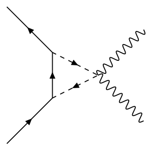
We write the total amplitude as
| (33) |
where is the fine structure constant and such that for the final and for the final state. The structure reflects the -wave nature of this amplitude, since this factor is nonzero only for the initial state configuration. Then all the contributions from the loop integrals in Fig. (11) are collected in , which we write as
| (34) |
Because of the term , the probabilities of having and photon final states are unequal (note that , and are, in general, complex functions), which is a potentially measurable effect of violation. The coefficients , and are given by
| (35) | ||||
| (36) | ||||
| (37) |
where is the mass for the internal scalars (here we have adopted a simplified notation, in the main text). We observe that if , we have such that the amplitude will not vanish but it will depend neither on the mixing angle nor on the -violation phase . However, as seen from (5), the -wave annihilation cross section is identically zero in this case. If the integral is complex (which is the case for both the and channels), the amplitudes of the and final states do not have the same magnitude, which leads to an asymmetry ratio as discussed in the main text. Here and are the same as and in Ref. [9]. They are related to the standard three-point scalar loop integrals through
| (38) | ||||
| (39) |
in which we follow the convention of LoopTools [38]. The analytic expressions for are
| (42) | ||||
| (43) |
where
| (44) |
We note that both the and terms are contained in the analytic expression in Refs.[8, 9], but the term is missing. Finally, we define the square of the total unpolarized amplitude as
| (45) |
and the total cross section is
| (46) |
where the factor accounts for the fact that the final state consists of identical particles.