∎

Simultaneous Approximation Terms for Multi-Dimensional Summation-by-Parts Operators

Journal: Journal of Scientific ComputingSome of the material presented in this article has also appeared in: Hicken J. E., Del Rey Fernández D. C and Zingg D. W. Simultaneous Approximation Terms for Multi-dimensional Summation-by-parts Operators, AIAA Aviation Conference (2016).

David C. Del Rey Fernández Jason E. Hicken David W. Zingg Affiliation: University of Toronto Institute for Aerospace Studies E-mail: dcdelrey@gmail.com Affiliation: Rensselaer Polytechnic Institute E-mail: hickej2@rpi.edu Affiliation: University of Toronto Institute for Aerospace Studies E-mail: dwz@oddjob.utias.utoronto.ca

Abstract

This paper is concerned with the accurate, conservative, and stable imposition of boundary conditions and inter-element coupling for multi-dimensional summation-by-parts (SBP) finite-difference operators. More precisely, the focus is on diagonal-norm SBP operators that are not based on tensor products and are applicable to unstructured grids composed of arbitrary elements. We show how penalty terms — simultaneous approximation terms (SATs) — can be adapted to discretizations based on multi-dimensional SBP operators to enforce boundary and interface conditions. A general SAT framework is presented that leads to conservative and stable discretizations of the variable-coefficient advection equation. This framework includes the case where there are no nodes on the boundary of the SBP element at which to apply penalties directly. This is an important generalization, because elements analogous to Legendre-Gauss collocation, i.e. without boundary nodes, typically have higher accuracy for the same number of degrees of freedom. Symmetric and upwind examples of the general SAT framework are created using a decomposition of the symmetric part of an SBP operator; these particular SATs enable the pointwise imposition of boundary and inter-element conditions. We illustrate the proposed SATs using triangular-element SBP operators with and without nodes that lie on the boundary. The accuracy, conservation, and stability properties of the resulting SBP-SAT discretizations are verified using linear advection problems with spatially varying divergence-free velocity fields.

1 Introduction

We are interested in high-order discretizations that obey the summation by parts (SBP) property. The SBP property mimics integration by parts, and it greatly facilitates the construction of high-order schemes that are conservative and provably stable (linearly and nonlinearly) [1, 2, 3]. We are, in addition, interested in the flexibility provided by SBP operators that do not have a standard polynomial basis representation. In principle, this flexibility can be used to optimize SBP operators in various ways. For example, their efficiency can be improved by reducing their spectral radius or decreasing the number of floating point operations per node.

SBP methods have predominantly been developed in the context of high-order finite difference methods [4, 5] where the nodal distribution in computational space is uniform; see the review papers [6, 7] and the references therein. While SBP methods have been extended in a number of ways, for example see [8, 9, 10, 11], the majority of these developments have been limited to one-dimensional operators that are applied to multi-dimensional problems using tensor-product operators in computational space. An interesting exception is the work by Nordström et al. [12], which presents a vertex-centered second-order-accurate finite-volume scheme with the SBP property on unstructured grids.

The tensor-product approach, while adequate for many applications, has limitations when applied to complex geometries and in the context of localized, anisotropic mesh adaptation. This motivates our interest in generalizing SBP operators to more general multi-dimensional subdomains, i.e. elements.

Building on the generalization in [9], we presented an SBP definition in [13] (see also [14]) that is suitable for arbitrary, bounded subdomains with piecewise smooth, orientable boundaries. For diagonal-norm¹¹ 1 The norm matrix can be viewed as a mass matrix. multi-dimensional SBP operators that are exact for polynomials of total degree $p$ , it was shown that the norm and corresponding nodes define a strong cubature rule that is exact for polynomials of degree $2p-1$ . This connection to cubature rules greatly simplifies the construction of SBP operators, since many suitable cubature rules have already been identified in the literature [15]. In this paper, we will only consider diagonal-norm operators.

SBP derivative operators do not inherently enforce boundary conditions or inter-element coupling. The majority of SBP-based discretizations rely on simultaneous approximation terms (SATs) [16, 17, 18, 19] to impose boundary conditions, as well as inter-element coupling when the solution space is discontinuous. SATs are terms that impose boundary data and inter-element coupling in a weak sense and lead to stable and conservative schemes without impacting the asymptotic order of the discretization.

In [13] we derived SATs for multidimensional diagonal-norm SBP operators and showed that the resulting discretizations are stable for the linear constant-coefficient advection equation. Indeed, for constant-coefficient advection these penalties are the strong-form equivalent of the boundary-integrated numerical flux functions used in [20]. The SATs described in [13] can theoretically accommodate variable-coefficient advection problems; however, they are not practical for this class of problem because new SBP operators would be needed whenever the variable coefficients change.

The multi-dimensional SBP operators in [13] were designed to have a unisolvent set of nodes on each face for the appropriate space of polynomials. This constraint was imposed, in part, to simplify the construction of pointwise SATs, but it increases the total number of nodes required for the SBP cubature. For example, the quadratic, cubic, and quartic SBP operators for the triangle require 7, 12, and 18 nodes, respectively, rather than the 6, 10, and 15 nodes necessary for a total-degree basis [13]. A similar trend is observed for tetrahedral elements. Given the quadratic complexity of matrix-vector multiplication, there is impetus to minimize the number of volume nodes. In addition, it is well known that strong cubature rules without boundary nodes tend to be more accurate than rules with boundary nodes for the same number of nodes [15].

In light of the limitations of the SATs used in [13], the objectives of the present work are to:

1.

generalize the SAT definition to accommodate multi-dimensional SBP operators that may not have a sufficient number of boundary nodes to construct adequate face cubature rules, including operators that have no boundary nodes, and;
2.

develop SATs that lead to provably stable and conservative schemes for variable coefficient partial differential equations (PDEs) in split form.

The remainder of the paper is organized as follows. After introducing some notation, Section 2 reviews the definition of multi-dimensional SBP operators from [13]. Section 3 demonstrates the decomposition of the symmetric component of the SBP-derivative operator by considering a set of auxiliary nodes on the boundary using interpolation/extrapolation operators and face cubature rules. In Sections 4 and 5 the general framework for construction of stable and conservative SATs is presented and two examples of SATs are discussed. In order to illustrate SATs on a concrete example, Section 6 presents two families of SBP operators for the triangle and describes how SATs are constructed for these operators. A numerical verification using the linear advection equation with a spatially varying divergence-free velocity field is given in Section 7, and conclusions are provided in Section 8.

2 Notation and review of multi-dimensional summation-by-parts operators

This work builds on [13], so similar notation is maintained for consistency. As in that work, we focus on two-dimensional operators to simplify the presentation. One notable difference between the present work and [13] is that we consider general (smooth) bijective mappings from physical to computational space. Domains and their boundaries in physical space are denoted with $\Omega$ and $\Gamma$ , respectively. The corresponding sets in computational space are given by $\hat{\Omega}$ and $\hat{\Gamma}$ . Physical-space coordinates are represented with $(x,y)\in\Omega$ , and the computational-space coordinates are given by $(\xi,\eta)\in\hat{\Omega}$ . Several definitions and theorems are limited to operators defined in the $\xi$ coordinate direction, since operators defined in the other directions are analogous.

Functions are denoted with capital letters with a script type; e.g., $\mathcal{U}(\xi,\eta,t)\in L^{2}(\hat{\Omega}\times[0,T])$ denotes a square-integrable function on the space-time domain $\hat{\Omega}\times[0,T]$ . Functions and operators are discretized on a set of $n$ nodes, $S_{\hat{\Omega}}=\left\{(\xi_{i},\eta_{i})\right\}_{i=1}^{n}\subset\hat{\Omega}$ . The restriction of a function to the nodes is a column vector that is represented using lower-case bold font. For example, in the case of $\mathcal{U}$ we would write

\bm{u}=\left[\mathcal{U}(\xi_{1},\eta_{1}),\dots,\mathcal{U}(\xi_{n},\eta_{n})\right]^{\mathrm{T}}.

A number of definitions and theorems rely on the monomial basis, defined below in (partial) order of nondecreasing degree.

\mathcal{P}_{k}(\xi,\eta)\equiv\xi^{i}\eta^{j-i},\qquad k=j(j+1)/2+i+1,\quad\forall\;j\in\{0,1,\ldots,p\},\quad i\in\{0,1,\ldots,j\}.

The cardinality of the monomial basis of total degree $p$ is denoted

N^{*}_{p}\equiv\binom{p+d}{d},

where $d$ is the spatial dimension; for $d=2$ this gives $N^{*}_{p}=(p+1)(p+2)/2$ . The monomials and their derivatives evaluated at the nodes are represented by the $n$ -vectors

	$\displaystyle\bm{p}_{k}$	$\displaystyle\equiv\left[\mathcal{P}_{k}(\xi_{1},\eta_{1}),\dots,\mathcal{P}_{k}(\xi_{n},\eta_{n})\right]^{\mathrm{T}},$
	$\displaystyle\text{and}\qquad\bm{p}_{k}^{\prime}$	$\displaystyle\equiv\left[\frac{\partial\mathcal{P}_{k}}{\partial\xi}(\xi_{1},\eta_{1}),\dots,\frac{\partial\mathcal{P}_{k}}{\partial\xi}(\xi_{n},\eta_{n})\right]^{\mathrm{T}}.$

We can now state the following definition of a multi-dimensional SBP operator that was proposed in [13]:

Definition 1

Two-dimensional summation-by-parts operator: Consider an open and bounded domain $\hat{\Omega}\subset\mathbb{R}^{2}$ with a piecewise-smooth boundary $\hat{\Gamma}$ . The matrix $\mathsf{D}_{\xi}$ is a degree $p$ SBP approximation to the first derivative $\frac{\partial}{\partial\xi}$ on the nodes $S_{\hat{\Omega}}=\left\{(\xi_{i},\eta_{i})\right\}_{i=1}^{n}$ if

I.

$\mathsf{D}_{\xi}\bm{p}_{k}=\bm{p}_{k}^{\prime},\qquad\forall\;k\in\{1,2,\ldots,N^{*}_{p}\}$ ;
II.

$\mathsf{D}_{\xi}=\mathsf{H}^{-1}\mathsf{Q}_{\xi}$ , where $\mathsf{H}$ is symmetric positive-definite; and

III.

$\mathsf{Q}_{\xi}=\mathsf{S}_{\xi}+\frac{1}{2}\mathsf{E}_{\xi}$ , where $\mathsf{S}_{\xi}^{\mathrm{T}}=-\mathsf{S}_{\xi}$ , $\mathsf{E}_{\xi}^{\mathrm{T}}=\mathsf{E}_{\xi}$ , and $\mathsf{E}_{\xi}$ satisfies

\bm{p}_{k}^{\mathrm{T}}\mathsf{E}_{\xi}\bm{p}_{m}=\displaystyle\oint_{\hat{\Gamma}}\mathcal{P}_{k}\mathcal{P}_{m}n_{\xi}\mathrm{d}\hat{\Gamma},\qquad\forall\;k,m\in\{1,2,\ldots,N^{*}_{r}\},

where $r\geq p$ , and $n_{\xi}$ is the $\xi$ component of $\bm{n}=\left[n_{\xi},n_{\eta}\right]^{\mathrm{T}}$ , the outward pointing unit normal on $\hat{\Gamma}$ .

A diagonal-norm SBP operator is one where $\mathsf{H}$ is a diagonal matrix. As mentioned in the Introduction, such diagonal-norm operators are closely linked to cubature rules and, under mild assumptions on a generalized Vandermonde matrix, the existence of a cubature implies the existence of an SBP operator [13]. Conversely, the norm matrix $\mathsf{H}$ is a cubature rule satisfying

\bm{p}_{k}^{\mathrm{T}}\mathsf{H}\bm{p}_{m}=\int_{\hat{\Omega}}\mathcal{P}_{k}\mathcal{P}_{m}\mathrm{d}\hat{\Omega},

where, at a minimum, $\mathsf{H}$ is of degree $2p-1$ , i.e. the above equality holds provided $\mathcal{P}_{k}\mathcal{P}_{m}$ is at most degree $2p-1$ . In addition, since $\mathsf{H}$ is symmetric positive definite, it defines the finite-dimensional norm (hence the name, norm matrix) that is a degree $2p-1$ approximation to the $L^{2}$ norm:

\|\bm{u}\|_{\mathsf{H}}^{2}\equiv\bm{u}^{\mathrm{T}}\mathsf{H}\bm{u}\approx\int_{\hat{\Omega}}\mathcal{U}^{2}\mathrm{d}\hat{\Omega}.

We use this norm frequently in the following stability analysis.

3 Decomposition of $\mathsf{E}_{\xi}$

The pointwise nature of SATs complicates their direct application to multi-dimensional SBP operators, which may not have any nodes on the boundary of their domain. Fortunately, as we show in this section, the $\mathsf{E}_{\xi}$ and $\mathsf{E}_{\eta}$ matrices of many multi-dimensional SBP operators can be decomposed in terms of nodes that lie on the boundary of $\hat{\Omega}$ . These auxiliary nodes provide a straightforward means of applying traditional SAT penalties.

In order to proceed, we introduce some assumptions regarding the reference element, $\hat{\Omega}$ , and its boundary, $\hat{\Gamma}$ .

Assumption 1

The reference element $\hat{\Omega}$ is a polygon, and its boundary $\hat{\Gamma}$ is piecewise linear with $\hat{\Gamma}=\bigcup_{j=1}^{\kappa}\hat{\Gamma}_{j}$ and $\bigcap_{j=1}^{\kappa}\hat{\Gamma}_{j}=\emptyset$ . Furthermore, for each $\hat{\Gamma}_{j}$ there exists a strong cubature rule, with nodes $S_{\hat{\Gamma}_{j}}=\{(\xi_{i}^{(j)},\eta_{i}^{(j)})\}_{i=1}^{n_{j}}$ and weights $\{b_{i}^{(j)}\}_{i=1}^{n_{j}}$ , that exactly integrates polynomial integrands of degree $q\geq 2r$ , where $r$ is the integer used in property III of Definition 1.

Remark 1

The assumption that the reference element is a polygon is reasonable; for example, the most common finite elements are polytopes in computational space.

Assumption 1 ensures that we can evaluate element boundary fluxes with sufficient accuracy in computational space. For example, the cubature rule for each $\hat{\Gamma}_{j}$ allows us to write

\int_{\hat{\Gamma}_{j}}\mathcal{P}_{k}(\xi,\eta)n_{\xi}\,\mathrm{d}\hat{\Gamma}=n_{\xi j}\sum_{i=1}^{n_{j}}b_{i}^{(j)}\mathcal{P}_{k}\left(\xi_{i}^{(j)},\eta_{i}^{(j)}\right),

for all polynomials $\mathcal{P}_{k}$ of total degree $q$ or less, where $q\geq 2r$ . A similar expression holds for fluxes in the $\eta$ direction. Note that $n_{\xi j}$ is constant over $\hat{\Gamma}_{j}$ , due to linearity, so it can be pulled outside the integral.

Our approach to imposing boundary and interface conditions pointwise is to interpolate/extrapolate the solution from the element nodes onto the cubature nodes $S_{\hat{\Gamma}_{j}}=\{(\xi_{i}^{(j)},\eta_{i}^{(j)}\}_{i=1}^{n_{j}}$ using operators $\mathsf{R}_{j}$ . To decompose $\mathsf{E}_{\xi}$ and $\mathsf{E}_{\eta}$ , these interpolation/extrapolation operators must be sufficiently accurate. Specifically,

\left(\mathsf{R}_{j}\bm{p}_{k}\right)_{i}=\mathcal{P}_{k}\left(\xi_{i}^{(j)},\eta_{i}^{(j)}\right),\quad i=1,2,\ldots,n_{j},\qquad\forall\;k\in\{1,2,\ldots,N^{*}_{r}\},

where $r\geq p$ .

We first prove that we can construct $\mathsf{E}_{\xi}$ that satisfy the requirements of Definition 1 using the interpolation/extrapolation operators, $\mathsf{R}$ , and the face-cubature rules from Assumption 1.

Theorem 1

Let Assumption 1 hold and let $S_{\hat{\Omega}}=\left\{\left(\xi_{i},\eta_{i}\right)\right\}_{i=1}^{n}$ be a given a nodal distribution on the domain $\hat{\Omega}$ . Then, a matrix $\mathsf{E}_{\xi}$ that satisfies the requirements of Definition 1 can be constructed as

\mathsf{E}_{\xi}=\sum_{j=1}^{\kappa}n_{\xi j}\mathsf{R}_{j}^{\mathrm{T}}\mathsf{B}_{j}\mathsf{R}_{j},

(1)

where $\mathsf{B}_{j}=\mydiag\left(b_{1}^{(j)},b_{2}^{(j)},\ldots,b_{n_{j}}^{(j)}\right)$ is a diagonal matrix holding the cubature weights for $\hat{\Gamma}_{j}$ , and $\mathsf{R}_{j}\in\mathbb{R}^{n_{j}\times n}$ is a degree $r\geq p$ interpolation/extrapolation operator from the nodes $S_{\hat{\Omega}}$ to the nodes of the reference boundary domain, $S_{\hat{\Gamma}_{j}}$ .

Proof

The terms $\mathsf{R}_{j}^{\mathrm{T}}\mathsf{B}_{j}\mathsf{R}_{j}$ are symmetric by construction. Therefore, we need only show that the accuracy conditions of Property III hold. Since the $\mathsf{R}_{j}$ are exact for degree $r\geq p$ polynomials, we have, $\forall\;k,m\in\{1,2,\ldots,N^{*}_{r}\}$ ,

	$\displaystyle\bm{p}_{k}^{\mathrm{T}}\tilde{\mathsf{E}}_{\xi}\bm{p}_{m}$	$\displaystyle=\sum_{j=1}^{\kappa}n_{\xi j}\bm{p}_{k}^{\mathrm{T}}\mathsf{R}_{j}^{\mathrm{T}}\mathsf{B}_{j}\mathsf{R}_{j}\bm{p}_{m}$
		$\displaystyle=\sum_{j=1}^{\kappa}n_{\xi j}\sum_{i=1}^{n_{j}}b_{i}^{(j)}\mathcal{P}_{k}\left(\xi_{i}^{(j)},\eta_{i}^{(j)}\right)\mathcal{P}_{m}\left(\xi_{i}^{(j)},\eta_{i}^{(j)}\right)$
		$\displaystyle=\sum_{j=1}^{\kappa}\int_{\hat{\Gamma}_{j}}\mathcal{P}_{k}\mathcal{P}_{m}n_{\xi j}\,\mathrm{d}\hat{\Gamma},$

where we have used the linearity of the mappings (see Assumption 1) and the fact that the product $\mathcal{P}_{k}\mathcal{P}_{m}$ has total degree less than or equal to $2r\leq q$ . The result follows by the additive property of integrals.∎

Next, we prove that we can construct a multi-dimensional SBP operator $\mathsf{D}_{\xi}$ from a given, sufficiently accurate, strong cubature rule and an $\mathsf{E}_{\xi}$ matrix that satisfies the requirements of Definition 1. For this result, we will need the degree $p$ (rectangular) Vandermonde matrix

\mathsf{V}\equiv\left[\bm{p}_{1},\bm{p}_{2},\dots,\bm{p}_{N^{*}_{p}}\right],

as well as the associated matrix containing the projection of the $\xi$ derivatives of the monomials

\mathsf{V}_{\xi}\equiv\left[\bm{p}_{1}^{\prime},\bm{p}_{2}^{\prime},\dots,\bm{p}_{N^{*}_{p}}^{\prime}\right].

Theorem 2

Let the diagonal elements of $\mathsf{H}$ and the nodes $S_{\hat{\Omega}}=\left\{\left(\xi_{i},\eta_{i}\right)\right\}_{i=1}^{n}$ define a degree $2p-1$ strong cubature rule on the domain $\hat{\Omega}$ . If the Vandermonde matrix, $\mathsf{V}$ , associated with the nodes $S_{\hat{\Omega}}$ has full column rank, and $\mathsf{E}_{\xi}\in\mathbb{R}^{n\times n}$ is symmetric and satisfies Property III of Definition 1, then there exists at least one degree $p$ SBP operator, $\mathsf{D}_{\xi}=\mathsf{H}^{-1}(\mathsf{S}_{\xi}+\frac{1}{2}\mathsf{E}_{\xi})$ , based on the given nodes $S_{\hat{\Omega}}$ and matrices $\mathsf{H}$ and $\mathsf{E}_{\xi}$ .

Proof

We must show that, for the given $\mathsf{H}$ and $\mathsf{E}_{\xi}$ , we can find a skew symmetric $\mathsf{S}_{\xi}$ that satisfies the accuracy conditions I. The SBP accuracy conditions can be recast as the following set of matrix conditions:

\mathsf{D}_{\xi}\overbrace{\left[\mathsf{V}\;\mathsf{W}\right]}^{\tilde{\mathsf{V}}}=\overbrace{\left[\mathsf{V}\;\mathsf{W}_{\xi}\right]}^{\tilde{\mathsf{V}}_{\xi}},

(2)

where $\mathsf{W}$ is a set of linearly independent vectors, of size $n\times(n-N^{*}_{p})$ , such that $\tilde{\mathsf{V}}$ is invertible, e.g., a basis for the null space of $\mathsf{V}$ . The matrix $\mathsf{W}_{\xi}$ is of size $n\times(n-N^{*}_{p})$ and is to be determined. Using (2) and the multi-dimensional SBP definition, we can solve for $\mathsf{S}_{\xi}$ as

\mathsf{S}_{\xi}=\mathsf{H}\tilde{\mathsf{V}}_{\xi}\tilde{\mathsf{V}}^{-1}-\frac{1}{2}\mathsf{E}_{\xi}.

(3)

What remains to be shown is that $\mathsf{S}_{\xi}$ can be constructed to be skew symmetric using $\mathsf{W}_{\xi}$ . Rather than doing so directly, we show that an associated matrix is skew symmetric; left and right multiplying (3) by $\tilde{\mathsf{V}}^{\mathrm{T}}$ and $\tilde{\mathsf{V}}$ , respectively, results in

\tilde{\mathsf{S}}_{\xi}\equiv\tilde{\mathsf{V}}^{\mathrm{T}}\mathsf{S}_{\xi}\tilde{\mathsf{V}}=\begin{bmatrix}\mathsf{V}^{\mathrm{T}}\mathsf{H}\mathsf{V}_{\xi}-\frac{1}{2}\mathsf{V}^{\mathrm{T}}\mathsf{E}_{\xi}\mathsf{V}&\mathsf{V}^{\mathrm{T}}\mathsf{H}\mathsf{W}_{\xi}-\frac{1}{2}\mathsf{V}^{\mathrm{T}}\mathsf{E}_{\xi}\mathsf{W}\\ \mathsf{W}^{\mathrm{T}}\mathsf{H}\mathsf{V}_{\xi}-\frac{1}{2}\mathsf{W}^{\mathrm{T}}\mathsf{E}_{\xi}\mathsf{V}&\mathsf{W}^{\mathrm{T}}\mathsf{H}\mathsf{W}_{\xi}-\frac{1}{2}\mathsf{W}^{\mathrm{T}}\mathsf{E}_{\xi}\mathsf{W}\end{bmatrix}.

(4)

If we can show that $\tilde{\mathsf{S}}_{\xi}$ is skew symmetric, this will imply skew symmetry for $\mathsf{S}_{\xi}$ .

We first show that the block $\tilde{\mathsf{S}}_{\xi}(1:N^{*}_{p},1:N^{*}_{p})$ is skew symmetric;

\tilde{\mathsf{S}}_{\xi}(1:N^{*}_{p},1:N^{*}_{p})+\tilde{\mathsf{S}}_{\xi}(1:N^{*}_{p},1:N^{*}_{p})^{\mathrm{T}}=\mathsf{V}^{\mathrm{T}}\mathsf{H}\mathsf{V}_{\xi}+\mathsf{V}_{\xi}^{\mathrm{T}}\mathsf{H}\mathsf{V}-\mathsf{V}^{\mathrm{T}}\mathsf{E}_{\xi}\mathsf{V}=0,

where we have used the compatibility conditions $\mathsf{V}^{\mathrm{T}}\mathsf{H}\mathsf{V}_{\xi}+\mathsf{V}_{\xi}^{\mathrm{T}}\mathsf{H}\mathsf{V}=\mathsf{V}^{\mathrm{T}}\mathsf{E}_{\xi}\mathsf{V}$ [13, 9, 5, 4].

Next, notice that the entries in the lower-left block $\tilde{\mathsf{S}}_{\xi}(N^{*}_{p}+1:n,1:N^{*}_{p})$ are fully specified by $\mathsf{V}$ , $\mathsf{W}$ , and $\mathsf{V}_{\xi}$ . To make the rest of $\tilde{\mathsf{S}}_{\xi}$ skew symmetric, we specify the columns of $\mathsf{W}_{\xi}$ in order to match the upper-right block to the (negative transposed) lower-left block and a zero lower-right block. In other words, for skew-symmetry we require that

\tilde{\mathsf{S}}_{\xi}(:,N^{*}_{p}+j)=\tilde{\mathsf{V}}^{\mathrm{T}}\mathsf{H}\mathsf{W}_{\xi}-\frac{1}{2}\tilde{\mathsf{V}}^{\mathrm{T}}\mathsf{E}_{\xi}\mathsf{W}=\begin{bmatrix}-\mathsf{V}_{\xi}^{\mathrm{T}}\mathsf{H}\mathsf{W}+\frac{1}{2}\mathsf{V}^{\mathrm{T}}\mathsf{E}_{\xi}\mathsf{W}\\ \mathsf{0}\end{bmatrix}.

Rearranging we have

\tilde{\mathsf{V}}^{\mathrm{T}}\mathsf{H}\mathsf{W}_{\xi}=\frac{1}{2}\tilde{\mathsf{V}}^{\mathrm{T}}\mathsf{E}_{\xi}\mathsf{W}+\begin{bmatrix}-\mathsf{V}_{\xi}^{\mathrm{T}}\mathsf{H}\mathsf{W}+\frac{1}{2}\mathsf{V}^{\mathrm{T}}\mathsf{E}_{\xi}\mathsf{W}\\ \mathsf{0}\end{bmatrix},

which we can solve for $\mathsf{W}_{\xi}$ , because $\tilde{\mathsf{V}}^{\mathrm{T}}\mathsf{H}$ is invertible. This particular $\mathsf{W}_{\xi}$ ensures that $\tilde{\mathsf{S}}_{\xi}$ is skew symmetric, and, therefore, guarantees that $\mathsf{S}_{\xi}$ is skew symmetric. ∎

Theorems 1 and 2 imply the following:

Corollary 1

If the hypotheses of Theorem 1 and 2 are met, then there exists at least one degree $p$ SBP operator whose $\mathsf{E}_{\xi}$ has the decomposition (1).

Remark 2

The implication of Corollary 1 is that $\mathsf{D}_{\xi}$ exist for which $\mathsf{E}_{\xi}$ is constructed as the sum of matrices, each of which is associated with a face $\hat{\Gamma}_{j}$ ; more importantly, it expresses these constituent matrices in terms of the face cubature points and the $\mathsf{R}_{j}$ operators, facilitating pointwise imposition of SATs.

4 Linear variable-coefficient PDEs

While the ideas presented in this paper can be used to construct SATs for PDEs in various forms, one of our goals is to develop SATs suitable for split forms of nonlinear PDEs. Such split forms can be used to prove nonlinear stability, for example of the Burgers and Euler equations, and more generally are related to the entropy stability theory in Refs. [21, 22, 1, 2, 3]. Moreover, such split-forms can be advantageous in improving robustness [23]. Therefore, in this section, we develop a general framework for constructing SATs to impose boundary and inter-element conditions weakly for multi-dimensional SBP operators in split form. We do so by examining the variable-coefficient linear advection equation in two dimensions in skew-symmetric form. We review the use of the energy method to prove stability for the continuous problem and then apply the same ideas to prove stability of the semi-discrete equations. The goal of this section is to determine a set of conditions that, if satisfied, lead to stable and conservative semi-discrete forms.

4.1 Stability and conservation of the variable-coefficient linear advection equation

Consider the divergence and skew-symmetric forms of the linear advection equation with a spatially varying velocity field, $\bm{\lambda}=\left[\lambda_{x},\lambda_{y}\right]^{\mathrm{T}}$ :

\begin{split}\frac{\partial\mathcal{U}}{\partial t}=&-\nabla\cdot\left(\bm{\lambda}\mathcal{U}\right)\\ =&-\frac{1}{2}\nabla\cdot\left(\bm{\lambda}\mathcal{U}\right)-\frac{1}{2}\bm{\lambda}\cdot\nabla\mathcal{U}-\frac{1}{2}\mathcal{U}\nabla\cdot\bm{\lambda},\end{split}

(5)

for all $(x,y)\in\Omega$ and $t\geq 0$ . The initial and boundary conditions are

	$\displaystyle\mathcal{U}(x,y,0)$	$\displaystyle=\mathcal{F}(x,y),$		$\displaystyle\forall\;(x,y)\in\Omega,$		(6)
	$\displaystyle\mathcal{U}(x,y,t)$	$\displaystyle=\mathcal{G}(x,y,t),$		$\displaystyle\forall\;(x,y)\in\Gamma^{-},\quad t\geq 0,$		(6)

respectively, where $\Gamma$ is subdivided into the inflow boundary,

\Gamma^{-}=\left\{(x,y)\in\Gamma\,|\,n_{x}\lambda_{x}+n_{y}\lambda_{y}<0\right\},

and the outflow boundary, $\Gamma^{+}=\Gamma\backslash\Gamma^{-}$ .

We use the energy method — applying a similar analysis to that in Ref. [24] to our two-dimensional problem — to prove that the problem defined by (5) and (6) is stable; those interested in further details are referred to the texts [25, 26]. Multiplying the divergence form of (5) by $\mathcal{U}$ and integrating in space results in

\int_{\Omega}\mathcal{U}\frac{\partial\mathcal{U}}{\partial t}\mathrm{d}\Omega=-\int_{\Omega}\left(\mathcal{U}\frac{\partial\lambda_{x}\mathcal{U}}{\partial x}+\mathcal{U}\frac{\partial\lambda_{y}\mathcal{U}}{\partial y}\right)\mathrm{d}\Omega.

(7)

Equation (7) can be expressed in two alternative forms: i) using the Leibniz rule on the left-hand side and the product rule on the right-hand side, or; ii) using the Leibniz rule on the left-hand side and expanding the derivative terms on the right-hand side. Adding these two alternative expressions leads to

\frac{\mathrm{d}\|\mathcal{U}\|^{2}}{\mathrm{d}t}=-\int_{\Omega}\left(\frac{\partial\lambda_{x}\mathcal{U}^{2}}{\partial x}+\frac{\partial\lambda_{y}\mathcal{U}^{2}}{\partial y}+\mathcal{U}^{2}\frac{\partial\lambda_{x}}{\partial x}+\mathcal{U}^{2}\frac{\partial\lambda_{y}}{\partial y}\right)\mathrm{d}\Omega.

(8)

Using integration by parts on the first two terms of the right-hand side of (8) leads to

\frac{\mathrm{d}\|\mathcal{U}\|^{2}}{\mathrm{d}t}=-\oint_{\Gamma}\mathcal{U}^{2}\left(n_{x}\lambda_{x}+n_{y}\lambda_{y}\right)\mathrm{d}\Gamma-\int_{\Omega}\mathcal{U}^{2}\left(\frac{\partial\lambda_{x}}{\partial x}+\frac{\partial\lambda_{y}}{\partial y}\right)\mathrm{d}\Omega.

(9)

Assuming that the divergence of $\bm{\lambda}$ is bounded, that is

\alpha=\max\limits_{(x,y)\in\Omega}\left(\frac{\partial\lambda_{x}}{\partial x}+\frac{\partial\lambda_{y}}{\partial y}\right)\leq\infty,

we have that

\int_{\Omega}\mathcal{U}^{2}\left(\frac{\partial\lambda_{x}}{\partial x}+\frac{\partial\lambda_{y}}{\partial y}\right)\mathrm{d}\Omega\leq\alpha\|\mathcal{U}\|^{2}.

The following inequality results from breaking up the surface integral in (9) into integrals over $\Gamma^{+}$ and $\Gamma^{-}$ , inserting the boundary condition, and making use of the above bound:

\begin{split}\frac{\mathrm{d}\|\mathcal{U}\|^{2}}{\mathrm{d}t}\leq&-\oint_{\Gamma^{+}}\mathcal{U}^{2}|n_{x}\lambda_{x}+n_{y}\lambda_{y}|\mathrm{d}\Gamma+\oint_{\Gamma^{-}}\mathcal{G}^{2}|n_{x}\lambda_{x}+n_{y}\lambda_{y}|\mathrm{d}\Gamma+\alpha\|\mathcal{U}\|^{2}\\ \leq&\oint_{\Gamma^{-}}\mathcal{G}^{2}|n_{x}\lambda_{x}+n_{y}\lambda_{y}|\mathrm{d}\Gamma+\alpha\|\mathcal{U}\|^{2}.\end{split}

(10)

We integrate (10) in time and apply the initial condition (see [25] pg. 94), resulting in the estimate

\begin{split}\|\mathcal{U}\|^{2}\leq\exp\left(\alpha t\right)\|\mathcal{F}\|^{2}+\int_{0}^{t}\exp\left(\alpha(t-\tau)\right)\beta(\tau)\mathrm{d}\tau,\\ \textrm{ where }\qquad\beta\equiv\oint_{\Gamma^{-}}\mathcal{G}^{2}|n_{x}\lambda_{x}+n_{y}\lambda_{y}|\mathrm{d}\Gamma.\end{split}

Thus, we see that the problem defined by (5) and (6) is stable in the sense of Hadamard, that is, the solution depends continuously on the data [25].

Remark 3

In the numerical experiments presented later, we consider the special case of (5) where the velocity is divergence free, $\nabla\cdot\bm{\lambda}=0$ , and the boundary conditions are periodic. Under these assumptions, starting from (8), the energy method results in

\frac{\mathrm{d}\|\mathcal{U}\|^{2}}{\mathrm{d}t}=0,

which shows that the energy is constant.

In addition to stability, we are interested in constructing schemes that are conservative. To understand the discrete conditions that will be imposed, it is useful to delineate the conditions on the continuous problem. The PDE (5) has an integral form representation given as

\frac{\mathrm{d}}{\mathrm{d}t}\int_{\tilde{\Omega}}\mathcal{U}\mathrm{d}\Omega+\oint_{\tilde{\Gamma}}\mathcal{U}\bm{n}\cdot\bm{\lambda}\mathrm{d}\Gamma=0,

(11)

where (11) holds for all arbitrary subdomains $\tilde{\Omega}\subset\Omega$ with piecewise smooth, orientable boundaries $\tilde{\Gamma}$ . Typically, the strong form (5) is discretized using SBP-SAT schemes; nevertheless, we would like our schemes to mimic (11) discretely on arbitrary domains composed of one or more elements.

4.2 The generic SBP-SAT semi-discretization

In this section, we present a generic SBP-SAT semi-discretization of (5), and then determine the general conditions on the SATs necessary to obtain an energy-stable, accurate, and conservative scheme. We focus on SATs for inter-element coupling — weak enforcement of boundary conditions is similar.

The domain $\Omega$ is partitioned into $E$ nonoverlapping elements: $\Omega=\bigcup_{e=1}^{E}\Omega_{e}$ . On each element $\Omega_{e}$ , the PDE (5) is mapped from physical coordinates to computational, or reference, coordinates. For a time-invariant transformation, this results in the following skew-symmetric form:

\frac{\partial\mathcal{J}\mathcal{U}}{\partial t}+\frac{1}{2}\frac{\partial\lambda_{\xi}\mathcal{U}}{\partial\xi}+\frac{1}{2}\frac{\partial\lambda_{\eta}\mathcal{U}}{\partial\eta}+\frac{\lambda_{\xi}}{2}\frac{\partial\mathcal{U}}{\partial\xi}+\frac{\lambda_{\eta}}{2}\frac{\partial\mathcal{U}}{\partial\eta}+\frac{\mathcal{U}}{2}\left(\frac{\partial\lambda_{\xi}}{\partial\xi}+\frac{\partial\lambda_{\eta}}{\partial\eta}\right)=0,

(12)

where

\lambda_{\xi}=\frac{\partial y}{\partial\eta}\lambda_{x}-\frac{\partial x}{\partial\eta}\lambda_{y},\quad\lambda_{\eta}=-\frac{\partial y}{\partial\xi}\lambda_{x}+\frac{\partial x}{\partial\xi}\lambda_{y},\quad\mathcal{J}=\frac{\partial x}{\partial\xi}\frac{\partial y}{\partial\eta}-\frac{\partial x}{\partial\eta}\frac{\partial y}{\partial\xi}.

To present and analyze the SATs, we consider the interface between two generic elements, labeled “left” and “right,” having solutions $\bm{u}_{L}$ and $\bm{u}_{R}$ , respectively; see Figure 1. Suppose the left and right elements have $\kappa_{L}$ and $\kappa_{R}$ faces, respectively. Then, without loss of generality, we can index the non-shared faces such that the $\mathsf{E}_{\xi L}$ and $\mathsf{E}_{\xi R}$ decompositions can be written as (see Theorem 1)

\mathsf{E}_{\xi L}=\sum_{j=1}^{\kappa_{L}-1}\mathsf{E}_{\xi L,j}+n_{\xi L}\mathsf{R}_{L}^{\mathrm{T}}\mathsf{B}_{L}\mathsf{R}_{L}\quad\text{and}\quad\mathsf{E}_{\xi R}=\sum_{j=1}^{\kappa_{R}-1}\mathsf{E}_{\xi R,j}+n_{\xi R}\mathsf{R}_{R}^{\mathrm{T}}\mathsf{B}_{R}\mathsf{R}_{R},

where the terms $n_{\xi L}\mathsf{R}_{L}^{\mathrm{T}}\mathsf{B}_{L}\mathsf{R}_{L}$ and $n_{\xi R}\mathsf{R}_{R}^{\mathrm{T}}\mathsf{B}_{R}\mathsf{R}_{R}$ correspond to the shared face. Similar expressions hold for $\mathsf{E}_{\eta L}$ and $\mathsf{E}_{\eta R}$ . In the following, we will focus on the shared face and will drop contributions from the remaining $\kappa_{L}-1$ faces on the left and $\kappa_{R}-1$ faces on the right, unless otherwise noted.

Figure 1: Illustration of two generic SBP elements and their common interface used for the analysis of SATs. The circles denote the volume nodes at which the solutions

\bm{u}_{L}

and

\bm{u}_{R}

are stored, and the black squares denote cubature nodes for the face; the latter are introduced in Section 3.

The SBP-SAT semi-discretization of (12) is given by

\frac{\mathrm{d}}{\mathrm{d}t}\left(\mathsf{J}_{L}\bm{u}_{L}\right)+\frac{1}{2}\mathsf{D}_{\xi L}\Lambda_{\xi L}\bm{u}_{L}+\frac{1}{2}\mathsf{D}_{\eta L}\Lambda_{\eta L}\bm{u}_{L}+\frac{1}{2}\Lambda_{\xi L}\mathsf{D}_{\xi L}\bm{u}_{L}+\frac{1}{2}\Lambda_{\eta L}\mathsf{D}_{\eta L}\bm{u}_{L}\\ +\frac{\mathsf{U}_{L}}{2}\left(\mathsf{D}_{\xi L}\Lambda_{\xi L}\bm{1}_{L}+\mathsf{D}_{\eta L}\Lambda_{\eta L}\bm{1}_{L}\right)=\underbrace{\frac{1}{2}\mathsf{H}_{L}^{-1}\left(\mathsf{M}^{\lambda_{\xi}}_{LL}\bm{u}_{L}-\mathsf{M}^{\lambda_{\xi}}_{LR}\bm{u}_{R}\right)}_{\bm{\mathrm{SAT}}_{L}},

(13)

on the left element and

\frac{\mathrm{d}}{\mathrm{d}t}\left(\mathsf{J}_{R}\bm{u}_{R}\right)+\frac{1}{2}\mathsf{D}_{\xi R}\Lambda_{\xi R}\bm{u}_{R}+\frac{1}{2}\mathsf{D}_{\eta R}\Lambda_{\eta R}\bm{u}_{R}+\frac{1}{2}\Lambda_{\xi R}\mathsf{D}_{\xi R}\bm{u}_{R}+\frac{1}{2}\Lambda_{\eta R}\mathsf{D}_{\eta R}\bm{u}_{R}\\ +\frac{\mathsf{U}_{R}}{2}\left(\mathsf{D}_{\xi R}\Lambda_{\xi R}\bm{1}_{R}+\mathsf{D}_{\eta R}\Lambda_{\eta R}\bm{1}_{R}\right)=\underbrace{\frac{1}{2}\mathsf{H}_{R}^{-1}\left(\mathsf{M}^{\lambda_{\xi}}_{RR}\bm{u}_{R}-\mathsf{M}^{\lambda_{\xi}}_{RL}\bm{u}_{R}\right)}_{\bm{\mathrm{SAT}}_{R}},

(14)

on the right element. These discretizations introduce several new matrices and vectors. For instance,

	$\displaystyle\Lambda_{\xi L}$	$\displaystyle=\textrm{diag}\left(\lambda_{\xi}(\xi_{1},\eta_{1}),\dots,\lambda_{\xi}(\xi_{n_{L}},\eta_{n_{L}})\right),$
	$\displaystyle\mathsf{U}_{L}$	$\displaystyle=\textrm{diag}\left(u_{L,1},\dots,u_{L,n_{L}}\right),$
	$\displaystyle\mathsf{J}_{L}$	$\displaystyle=\textrm{diag}\left(\mathcal{J}(\xi_{1},\eta_{1}),\dots,\mathcal{J}(\xi_{n_{L}},\eta_{n_{L}})\right),$

are diagonal matrices, where $n_{L}$ is the number of nodes in the left element. Similar definitions hold for $\Lambda_{\eta L}$ , $\Lambda_{\xi R}$ , $\Lambda_{\eta R}$ , $\mathsf{U}_{R}$ , and $\mathsf{J}_{R}$ . In addition, $\bm{1}_{L}\in\mathbb{R}^{n_{L}}$ and $\bm{1}_{R}\in\mathbb{R}^{n_{R}}$ are constant vectors with entries equal to one.

The matrices $\mathsf{M}^{\lambda_{\xi}}_{LL}\in\mathbb{R}^{n_{L}\times n_{L}}$ , $\mathsf{M}^{\lambda_{\xi}}_{LR}\in\mathbb{R}^{n_{L}\times n_{R}}$ , $\mathsf{M}^{\lambda_{\xi}}_{RR}\in\mathbb{R}^{n_{R}\times n_{R}}$ , and $\mathsf{M}^{\lambda_{\xi}}_{RL}\in\mathbb{R}^{n_{R}\times n_{L}}$ depend on the spatially varying field $\bm{\lambda}_{\xi}=[\lambda_{\xi},\lambda_{\eta}]^{\mathrm{T}}$ , in general, and this dependence is reflected in the notation. It is these four SAT matrices that we seek to constrain using stability, accuracy, and conservation conditions.

4.2.1 Stability

We begin by determining the condition imposed by stability on the SAT matrices. The energy method applied to (13) and (14) consists of multiplying the equations by $\bm{u}_{L}^{\mathrm{T}}\mathsf{H}_{L}$ and $\bm{u}_{R}^{\mathrm{T}}\mathsf{H}_{R}$ , respectively, and adding the resulting expressions. After cancellation, and using the fact that $\bm{u}^{\mathrm{T}}\mathsf{H}\frac{\mathrm{d}\mathsf{J}\bm{u}}{\mathrm{d}t}=\frac{1}{2}\frac{\mathrm{d}\bm{u}^{\mathrm{T}}\mathsf{H}\mathsf{J}\bm{u}}{\mathrm{d}t}$ , we find

\frac{\mathrm{d}}{\mathrm{d}t}\left(\bm{u}_{L}^{\mathrm{T}}\mathsf{H}_{L}\mathsf{J}_{L}\bm{u}_{L}+\bm{u}_{R}^{\mathrm{T}}\mathsf{H}_{R}\mathsf{J}_{R}\bm{u}_{R}\right)=\\ -\bm{u}_{L}^{\mathrm{T}}\mathsf{U}_{L}\mathsf{H}_{L}\left(\mathsf{D}_{\xi L}\Lambda_{\xi L}\bm{1}_{L}+\mathsf{D}_{\eta L}\Lambda_{\eta L}\bm{1}_{L}\right)-\bm{u}_{R}^{\mathrm{T}}\mathsf{U}_{R}\mathsf{H}_{R}\left(\mathsf{D}_{\xi R}\Lambda_{\xi R}\bm{1}_{R}+\mathsf{D}_{\eta R}\Lambda_{\eta R}\bm{1}_{R}\right)\\ -\bm{u}_{L}^{\mathrm{T}}\mathsf{R}_{L}^{\mathrm{T}}\mathsf{B}_{L}\mathsf{R}_{L}\mathsf{\Lambda}_{L}\bm{u}_{L}+\bm{u}_{L}^{\mathrm{T}}\mathsf{M}^{\lambda_{\xi}}_{LL}\bm{u}_{L}-\bm{u}_{L}^{\mathrm{T}}\mathsf{M}^{\lambda_{\xi}}_{LR}\bm{u}_{R}\\ -\bm{u}_{R}^{\mathrm{T}}\mathsf{R}_{R}^{\mathrm{T}}\mathsf{B}_{R}\mathsf{R}_{R}\mathsf{\Lambda}_{R}\bm{u}_{R}+\bm{u}_{R}^{\mathrm{T}}\mathsf{M}^{\lambda_{\xi}}_{RR}\bm{u}_{R}-\bm{u}_{R}^{\mathrm{T}}\mathsf{M}^{\lambda_{\xi}}_{RL}\bm{u}_{L},

(15)

where

\mathsf{\Lambda}_{L}=n_{\xi L}\Lambda_{\xi L}+n_{\eta L}\Lambda_{\eta L}\qquad\text{and}\qquad\mathsf{\Lambda}_{R}=n_{\xi R}\Lambda_{\xi R}+n_{\eta R}\Lambda_{\eta R}.

As explained earlier, we have retained only those boundary matrices corresponding to the common face shared by the left and right elements. The terms corresponding to the remaining faces have been dropped to simplify the presentation.

We treat the first terms on the right, i.e. the terms on the second line of (15), in much the same way as we did for the continuous analysis. In particular, assuming the coordinate transformation is differentiable and has a bounded and nonzero Jacobian, we have

	$\displaystyle-\bm{u}_{L}^{\mathrm{T}}\mathsf{U}_{L}\mathsf{H}_{L}\left(\mathsf{D}_{\xi L}\Lambda_{\xi L}\bm{1}_{L}+\mathsf{D}_{\eta L}\Lambda_{\eta L}\bm{1}_{L}\right)$	$\displaystyle\leq\gamma_{L}\\|\bm{u}_{L}\\|_{\tilde{\mathsf{H}}_{L}}^{2},$
	$\displaystyle-\bm{u}_{R}^{\mathrm{T}}\mathsf{U}_{R}\mathsf{H}_{R}\left(\mathsf{D}_{\xi R}\Lambda_{\xi R}\bm{1}_{R}+\mathsf{D}_{\eta R}\Lambda_{\eta R}\bm{1}_{R}\right)$	$\displaystyle\leq\gamma_{R}\\|\bm{u}_{R}\\|_{\tilde{\mathsf{H}}_{R}}^{2}$

where

\begin{split}&\gamma_{L}=\max\limits_{i\in[1,n_{L}]}\left[\mathsf{J}_{L}^{-1}\left(\mathsf{D}_{\xi L}\Lambda_{\xi L}\bm{1}_{L}+\mathsf{D}_{\eta L}\Lambda_{\eta L}\bm{1}_{L}\right)\right]_{i},\\ &\gamma_{R}=\max\limits_{i\in[1,n_{R}]}\left[\mathsf{J}_{R}^{-1}\left(\mathsf{D}_{\xi R}\Lambda_{\xi R}\bm{1}_{R}+\mathsf{D}_{\eta R}\Lambda_{\eta R}\bm{1}_{R}\right)\right]_{i},\end{split}

and we have defined new norms $\tilde{\mathsf{H}}_{L}=\bm{u}_{L}^{\mathrm{T}}\mathsf{H}_{L}\mathsf{J}_{L}\bm{u}_{L}$ , $\tilde{\mathsf{H}}_{R}=\bm{u}_{R}^{\mathrm{T}}\mathsf{H}_{R}\mathsf{J}_{R}\bm{u}_{R}$ . Using these bounds in (15), and grouping the terms involving the SAT matrices, we obtain

\frac{\mathrm{d}}{\mathrm{d}t}\left(\|\bm{u}_{L}\|_{\tilde{\mathsf{H}}_{L}}^{2}+\|\bm{u}_{R}\|_{\tilde{\mathsf{H}}_{R}}^{2}\right)\leq C\left(\|\bm{u}_{L}\|_{\tilde{\mathsf{H}}_{L}}^{2}+\|\bm{u}_{R}\|_{\tilde{\mathsf{H}}_{R}}^{2}\right)\\ -\begin{bmatrix}\bm{u}_{L}^{\mathrm{T}}&\bm{u}_{R}^{\mathrm{T}}\end{bmatrix}\begin{bmatrix}\mathsf{R}_{L}^{\mathrm{T}}\mathsf{B}_{L}\mathsf{R}_{L}\mathsf{\Lambda}_{L}-\mathsf{M}^{\lambda_{\xi}}_{LL}&\mathsf{M}^{\lambda_{\xi}}_{LR}\\ \mathsf{M}^{\lambda_{\xi}}_{RL}&\mathsf{R}_{R}^{\mathrm{T}}\mathsf{B}_{R}\mathsf{R}_{R}\mathsf{\Lambda}_{R}-\mathsf{M}^{\lambda_{\xi}}_{RR}\end{bmatrix}\begin{bmatrix}\bm{u}_{L}\\ \bm{u}_{R}\end{bmatrix},

(16)

for $C=\max(\gamma_{L},\gamma_{R})$ .

In order to bound the solution in terms of the initial and boundary conditions, the matrix in the right-hand side must be must be negative semi-definite. This motivates the first condition on the SAT matrices.

Condition 1 (Stability)

The matrices $\mathsf{M}^{\lambda_{\xi}}_{LL}$ , $\mathsf{M}^{\lambda_{\xi}}_{LR}$ , $\mathsf{M}^{\lambda_{\xi}}_{RR}$ , and $\mathsf{M}^{\lambda_{\xi}}_{RL}$ must be such that

\begin{bmatrix}\mathsf{R}_{L}^{\mathrm{T}}\mathsf{B}_{L}\mathsf{R}_{L}\mathsf{\Lambda}_{L}-\mathsf{M}^{\lambda_{\xi}}_{LL}&\mathsf{M}^{\lambda_{\xi}}_{LR}\\ \mathsf{M}^{\lambda_{\xi}}_{RL}&\mathsf{R}_{R}^{\mathrm{T}}\mathsf{B}_{R}\mathsf{R}_{R}\mathsf{\Lambda}_{R}-\mathsf{M}^{\lambda_{\xi}}_{RR}\end{bmatrix}

is positive semi-definite for all $\mathsf{\Lambda}_{L}$ and $\mathsf{\Lambda}_{R}$ .

4.2.2 Accuracy

In order to maintain the accuracy of the base scheme, the SATs must add terms that are of the order of the discretization. The required conditions are therefore given by

Condition 2 (Accuracy)

The matrices $\mathsf{M}^{\lambda_{\xi}}_{LL}$ , $\mathsf{M}^{\lambda_{\xi}}_{LR}$ , $\mathsf{M}^{\lambda_{\xi}}_{RR}$ , and $\mathsf{M}^{\lambda_{\xi}}_{RL}$ must be such that

	$\displaystyle\mathsf{H}_{L}^{-1}\left(\mathsf{M}^{\lambda_{\xi}}_{LL}\bm{v}_{L}-\mathsf{M}^{\lambda_{\xi}}_{LR}\bm{v}_{R}\right)$	$\displaystyle=\mathcal{O}(h^{\tilde{p}}),$
	$\displaystyle\mathsf{H}_{R}^{-1}\left(\mathsf{M}^{\lambda_{\xi}}_{RR}\bm{v}_{R}-\mathsf{M}^{\lambda_{\xi}}_{RL}\bm{v}_{L}\right)$	$\displaystyle=\mathcal{O}(h^{\tilde{p}}),$

where $h$ is an appropriate measure for the linear dimension of the shared face, and $\bm{v}_{L}$ and $\bm{v}_{R}$ are the projection, onto the nodes of the left and right domains in physical space, of some continuous function $\mathcal{V}(x,y)$ , and $\tilde{p}\geq p$ .

We will have more to say about the above accuracy condition in the context of specific examples of SATs in Section 5.

4.2.3 Conservation

In order to determine the constraints on the SAT matrices such that the scheme is conservative, we multiply (13) by $\bm{1}_{L}^{\mathrm{T}}\mathsf{H}_{L}$ , and (14) by $\bm{1}_{R}^{\mathrm{T}}\mathsf{H}_{R}$ and sum the expressions; this operation is the discrete analogue of integrating the PDE over the volume consisting of both elements, i.e., $\tilde{\Omega}$ in (11). Simplifying the result we obtain

\frac{\mathrm{d}}{\mathrm{d}t}\left(\bm{1}_{L}^{\mathrm{T}}\mathsf{H}_{L}\mathsf{J}_{L}\bm{u}_{L}+\bm{1}_{R}^{\mathrm{T}}\mathsf{H}_{R}\mathsf{J}_{R}\bm{u}_{R}\right)=\\ \frac{1}{2}\left[-\bm{1}_{L}^{\mathrm{T}}\mathsf{R}_{L}\mathsf{B}_{L}\mathsf{R}_{L}\mathsf{\Lambda}_{L}\bm{u}_{L}-\bm{1}_{L}^{\mathrm{T}}\mathsf{\Lambda}_{L}\mathsf{R}_{L}^{\mathrm{T}}\mathsf{B}_{L}\mathsf{R}_{L}+\bm{1}_{L}^{\mathrm{T}}\mathsf{M}^{\lambda_{\xi}}_{LL}-\bm{1}_{R}^{\mathrm{T}}\mathsf{M}^{\lambda_{\xi}}_{RL}\right]\bm{u}_{L},\\ +\frac{1}{2}\left[-\bm{1}_{R}^{\mathrm{T}}\mathsf{R}_{R}^{\mathrm{T}}\mathsf{B}_{R}\mathsf{R}_{R}\mathsf{\Lambda}_{R}\bm{u}_{R}-\bm{1}_{R}^{\mathrm{T}}\mathsf{\Lambda}_{R}\mathsf{R}_{R}^{\mathrm{T}}\mathsf{B}_{R}\mathsf{R}_{R}+\bm{1}_{R}^{\mathrm{T}}\mathsf{M}^{\lambda_{\xi}}_{RR}-\bm{1}_{L}^{\mathrm{T}}\mathsf{M}^{\lambda_{\xi}}_{LR}\right]\bm{u}_{R}.

For conservation, we want the right-hand side to vanish for arbitrary $\bm{u}_{L}$ and $\bm{u}_{R}$ . Thus, after rearranging the right-hand side, we arrive at the third, and final, condition on the SAT matrices.

Condition 3 (Conservation)

The matrices $\mathsf{M}^{\lambda_{\xi}}_{LL}$ , $\mathsf{M}^{\lambda_{\xi}}_{LR}$ , $\mathsf{M}^{\lambda_{\xi}}_{RR}$ , and $\mathsf{M}^{\lambda_{\xi}}_{RL}$ must be such that

\left[\bm{1}_{L}^{\mathrm{T}}\left(\mathsf{M}^{\lambda_{\xi}}_{LL}-\mathsf{R}_{L}^{\mathrm{T}}\mathsf{B}_{L}\mathsf{R}_{L}\mathsf{\Lambda}_{L}\right)-\bm{1}_{R}^{\mathrm{T}}\mathsf{M}^{\lambda_{\xi}}_{RL}\right]\bm{u}_{L}\\ -\left[\bm{1}_{R}^{\mathrm{T}}\left(-\mathsf{M}^{\lambda_{\xi}}_{RR}+\mathsf{R}_{R}^{\mathrm{T}}\mathsf{B}_{R}\mathsf{R}_{R}\mathsf{\Lambda}_{R}\right)+\bm{1}_{L}^{\mathrm{T}}\mathsf{M}^{\lambda_{\xi}}_{LR}\right]\bm{u}_{R}\\ =\left(\mathsf{R}_{L}\mathsf{\Lambda}_{L}\bm{1}_{L}\right)^{\mathrm{T}}\mathsf{B}_{L}\mathsf{R}_{L}\bm{u}_{L}+\left(\mathsf{R}_{R}\mathsf{\Lambda}_{R}\bm{1}_{R}\right)^{\mathrm{T}}\mathsf{B}_{R}\mathsf{R}_{R}\bm{u}_{R}

for all $\bm{u}_{L}$ , $\bm{u}_{R}$ , $\mathsf{\Lambda}_{L}$ , $\mathsf{\Lambda}_{R}$ .

In the above condition, we have left the conservation conditions coupled and dependent on the solution as this is the typical situation for numerical fluxes used for nonlinear problems. We elaborate further on the conservation condition below.

4.3 Divergence-free advection field

We conclude Section 4 by investigating the special case of a divergence-free advection field in the variable-coefficient problem (5), i.e., $\nabla\cdot\bm{\lambda}=0$ . This case is of practical interest, because it arises in the incompressible Navier-Stokes and Maxwell’s equations. We also use this case to verify the theory for scalar variable-coefficient equations in Section 7.

In the divergence-free case, the skew-symmetric form of the PDE (5) simplifies to

\frac{\partial\mathcal{U}}{\partial t}=-\frac{1}{2}\nabla\cdot\left(\bm{\lambda}\mathcal{U}\right)-\frac{1}{2}\bm{\lambda}\cdot\nabla\mathcal{U},

(17)

and the SBP-SAT semi-discretization of (17) on the left element becomes

\frac{\mathrm{d}}{\mathrm{d}t}\left(\mathsf{J}_{L}\bm{u}_{L}\right)+\frac{1}{2}\mathsf{D}_{\xi L}\Lambda_{\xi L}\bm{u}_{L}+\frac{1}{2}\mathsf{D}_{\eta L}\Lambda_{\eta L}\bm{u}_{L}+\frac{1}{2}\Lambda_{\xi L}\mathsf{D}_{\xi L}\bm{u}_{L}+\frac{1}{2}\Lambda_{\eta L}\mathsf{D}_{\eta L}\bm{u}_{L}\\ =\frac{1}{2}\mathsf{H}_{L}^{-1}\left(\mathsf{M}^{\lambda_{\xi}}_{LL}\bm{u}_{L}-\mathsf{M}^{\lambda_{\xi}}_{LR}\bm{u}_{R}\right).

(18)

The semi-discretization on the right element is similar.

It is straightforward to show that the stability and accuracy conditions remain the same in the divergence-free case. However, the conservation condition is modified:

Condition 3^′ (Divergence-Free Conservation)

For the SBP-SAT semi-discretization of (17), the matrices $\mathsf{M}^{\lambda_{\xi}}_{LL}$ , $\mathsf{M}^{\lambda_{\xi}}_{LR}$ , $\mathsf{M}^{\lambda_{\xi}}_{RR}$ , and $\mathsf{M}^{\lambda_{\xi}}_{RL}$ must be such that

\left[\bm{1}_{L}^{\mathrm{T}}\left(\mathsf{M}^{\lambda_{\xi}}_{LL}-\mathsf{R}_{L}^{\mathrm{T}}\mathsf{B}_{L}\mathsf{R}_{L}\mathsf{\Lambda}_{L}\right)-\bm{1}_{R}^{\mathrm{T}}\mathsf{M}^{\lambda_{\xi}}_{RL}\right]\bm{u}_{L}\\ -\left[\bm{1}_{R}^{\mathrm{T}}\left(-\mathsf{M}^{\lambda_{\xi}}_{RR}+\mathsf{R}_{R}^{\mathrm{T}}\mathsf{B}_{R}\mathsf{R}_{R}\mathsf{\Lambda}_{R}\right)+\bm{1}_{L}^{\mathrm{T}}\mathsf{M}^{\lambda_{\xi}}_{LR}\right]\bm{u}_{R}=\\ \bm{1}_{L}^{\mathrm{T}}\left(\Lambda_{\xi L}\mathsf{Q}_{\xi L}+\Lambda_{\eta L}\mathsf{Q}_{\eta L}\right)\bm{u}_{L}+\bm{1}_{R}^{\mathrm{T}}\left(\Lambda_{\xi R}\mathsf{Q}_{\xi R}+\Lambda_{\eta L}\mathsf{Q}_{\eta R}\right)\bm{u}_{R}

for all $\bm{u}_{L}$ , $\bm{u}_{R}$ , $\Lambda_{\xi L}$ , $\Lambda_{\eta L}$ , $\Lambda_{\xi R}$ , and $\Lambda_{\eta R}$ .

Note that the right-hand side of the divergence-free conservation condition involves $\mathsf{Q}_{\xi}$ and $\mathsf{Q}_{\eta}$ .

5 Concrete examples of SATs: symmetric and upwind SATs

The SATs presented in Section 4 offer significant generality, but they are also somewhat abstract. In this section, we present two concrete examples of SATs — symmetric and upwind — for multidimensional SBP discretizations, and we show that these SATs satisfy Conditions 1–3 for stability, conservation, and accuracy.

The proposed symmetric and upwind SATs require the following assumption that constrains the face-cubature rules and coordinate transformations of adjacent elements.

Assumption 2

The cubature rule of the face shared by adjacent elements has the same number of nodes, $\nu$ , in both reference spaces. In addition, the coordinate transformations in the adjacent elements continuously map their respective face-cubature nodes to the same locations in physical space. For example, in the case of the left and right elements we have

x\left(\xi_{L,i},\eta_{L,i}\right)=x\left(\xi_{R,i},\eta_{R,i}\right)\quad\text{and}\quad y\left(\xi_{L,i},\eta_{L,i}\right)=y\left(\xi_{R,i},\eta_{R,i}\right),\qquad\forall\;i=1,2,\ldots,\nu,

where $\left(\xi_{L,i},\eta_{L,i}\right)$ and $\left(\xi_{R,i},\eta_{R,i}\right)$ denote the $i$ th face-cubature points on the left and right elements, respectively. Furthermore, the scaled face-normal vectors, based on the coordinate transformations along the shared face, are equal and opposite at the cubature nodes:

b_{L,i}\left[\mathcal{J}\left(n_{\xi}\nabla\xi+n_{\eta}\nabla\eta\right)\right]_{L,i}=-b_{R,i}\left[\mathcal{J}\left(n_{\xi}\nabla\xi+n_{\eta}\nabla\eta\right)\right]_{R,i},\qquad\forall\;i=1,2,\ldots,\nu,

(19)

where $b_{L,i}$ and $b_{R,i}$ denote the $i$ th face-cubature weights on the left and right elements, respectively.

Remark 4

In principle, the cubature rules for the shared face could use a different number of nodes on the left and right elements, but this case is beyond the scope of the current work.

Remark 5

Equation (19) is satisfied by isoparametric and subparametric coordinate transformations that use the same (possibly scaled) cubature rule on each face.

Let $\lambda_{n}=\lambda_{\xi}n_{\xi}+\lambda_{\eta}n_{\eta}$ be the advection velocity normal to the shared face. Then, assuming that $\lambda_{x}$ and $\lambda_{y}$ are continuous, one can use (19) and the definitions of $\lambda_{\xi}$ and $\lambda_{\eta}$ to show that

b_{L,i}\left(\lambda_{n}\right)_{L,i}=-b_{R,i}\left(\lambda_{n}\right)_{R,i},\qquad\forall\;i=1,2,\ldots,\nu.

(20)

In other words, the cubature-scaled advection velocity normal to the face is equal in magnitude and opposite in direction at the coincident nodes along the face. We use (20) to define the diagonal $\nu\times\nu$ matrix

\mathsf{B}_{\lambda}=\mathsf{B}_{L}\mathsf{\Lambda}_{\hat{\Gamma},L}=\mathsf{B}_{R}\mathsf{\Lambda}_{\hat{\Gamma},R}

(21)

where

\mathsf{\Lambda}_{\hat{\Gamma},L}=\mydiag\left[\left(\lambda_{n}\right)_{L,1},\ldots,\left(\lambda_{n}\right)_{L,\nu}\right],\qquad\mathsf{\Lambda}_{\hat{\Gamma},R}=-\mydiag\left[\left(\lambda_{n}\right)_{R,1},\ldots,\left(\lambda_{n}\right)_{R,\nu}\right].

$\mathsf{B}_{\lambda}$ will play a central role in defining the symmetric and upwind SATs below.

Remark 6

Using (20) to define $\mathsf{B}_{\lambda}$ simplifies the proof of accuracy for the symmetric and upwind SATs, but it is important to emphasize that neither (20) nor (19) are necessary for stability, accuracy, or conservation. Conditions 1–3 will still hold as long as $\mathsf{B}_{\lambda}$ agrees with (20) on the order of the discretization and satisfies (24) below. This is important, because nonlinear problems will not satisfy (20) due to jumps in $\lambda_{x}$ and $\lambda_{y}$ across elements.

5.1 Symmetric SATs

Symmetric SATs are constructed by defining

	$\displaystyle\mathsf{M}^{\lambda_{\xi}}_{LL}$	$\displaystyle=\mathsf{R}_{L}^{\mathrm{T}}\mathsf{B}_{L}\mathsf{R}_{L}\mathsf{\Lambda}_{L},\qquad$	$\displaystyle\mathsf{M}^{\lambda_{\xi}}_{LR}$	$\displaystyle=\mathsf{R}_{L}^{\mathrm{T}}\mathsf{B}_{\lambda}\mathsf{R}_{R},$		(22)
	$\displaystyle\mathsf{M}^{\lambda_{\xi}}_{RR}$	$\displaystyle=\mathsf{R}_{R}^{\mathrm{T}}\mathsf{B}_{R}\mathsf{R}_{R}\mathsf{\Lambda}_{R},\qquad$	$\displaystyle\mathsf{M}^{\lambda_{\xi}}_{RL}$	$\displaystyle=-\mathsf{R}_{R}^{\mathrm{T}}\mathsf{B}_{\lambda}\mathsf{R}_{L}.$		(22)

Based on these matrices, symmetric SATs for (13) and (14) are given by

	$\displaystyle 2\mathsf{H}_{L}\bm{\mathrm{SAT}}_{L,\mathrm{sym}}$	$\displaystyle=\mathsf{R}_{L}^{\mathrm{T}}\mathsf{B}_{L}\mathsf{R}_{L}\mathsf{\Lambda}_{L}\bm{u}_{L}-\mathsf{R}_{L}^{\mathrm{T}}\mathsf{B}_{\lambda}\mathsf{R}_{R}\bm{u}_{R},$		(23)
	$\displaystyle 2\mathsf{H}_{R}\bm{\mathrm{SAT}}_{R,\mathrm{sym}}$	$\displaystyle=\mathsf{R}_{R}^{\mathrm{T}}\mathsf{B}_{R}\mathsf{R}_{R}\mathsf{\Lambda}_{R}\bm{u}_{R}+\mathsf{R}_{R}^{\mathrm{T}}\mathsf{B}_{\lambda}\mathsf{R}_{L}\bm{u}_{L},$		(23)

Theorem 3

The symmetric SATs (23) satisfy the stability and accuracy Conditions 1 and 2. In addition, they satisfy the conservation Condition 3 provided

\bm{1}_{\hat{\Gamma}}^{\mathrm{T}}\mathsf{B}_{\lambda}\left(\mathsf{R}_{L}\bm{u}_{L}-\mathsf{R}_{R}\bm{u}_{R}\right)=\left(\mathsf{R}_{L}\mathsf{\Lambda}_{L}\bm{1}_{L}\right)^{\mathrm{T}}\mathsf{B}_{L}\mathsf{R}_{L}\bm{u}_{L}+\left(\mathsf{R}_{R}\mathsf{\Lambda}_{R}\bm{1}_{R}\right)^{\mathrm{T}}\mathsf{B}_{R}\mathsf{R}_{R}\bm{u}_{R}

(24)

for all $\bm{u}_{L}$ , $\bm{u}_{R}$ , $\mathsf{\Lambda}_{L}$ , $\mathsf{\Lambda}_{R}$ , where $\bm{1}_{\hat{\Gamma}}$ is a vector of ones of length $\nu$ .

Proof

It is easy to see that the symmetric SAT matrices (22) lead to a skew-symmetric matrix in Condition 1, which implies that the SATs (23) are stable.

To prove that the symmetric SATs satisfy the accuracy condition, we show that they vanish for all polynomial face-normal fluxes, $\left(\lambda_{\xi}n_{\xi}+\lambda_{\eta}n_{\eta}\right)\mathcal{U}$ , of total degree $p$ or less on the reference domain. We do this for the left-element SAT only, since the proof is analogous for the right-element SAT.

Let $\mathsf{\Lambda}_{L}\bm{u}_{L}\equiv\bm{p}_{k,L}$ be the face-normal polynomial flux evaluated at the SBP nodes of the left element (in reference space) — where we consider all $\mathsf{\Lambda}_{L}$ and $\bm{u}_{L}$ that satisfy this definition — and let $\bm{p}_{k,\hat{\Gamma}_{L}}$ be the same polynomial evaluated at the face-cubature points on the left element. Then, we consider those states on the right element such that

\mathsf{\Lambda}_{\hat{\Gamma},L}(\mathsf{R}_{R}\bm{u}_{R})=\bm{p}_{k,\hat{\Gamma}_{L}}.

Note that such states $\bm{u}_{R}$ exist provided $\mathsf{\Lambda}_{\hat{\Gamma},L}\mathsf{R}_{R}$ is full rank. The vector $\bm{p}_{k,\hat{\Gamma}_{L}}$ defines the “boundary” flux for which we must show the left SAT vanishes. We have

	$\displaystyle\mathsf{R}_{L}^{\mathrm{T}}\mathsf{B}_{L}\mathsf{R}_{L}\mathsf{\Lambda}_{L}\bm{u}_{L}-\mathsf{R}_{L}^{\mathrm{T}}\mathsf{B}_{\lambda}\mathsf{R}_{R}\bm{u}_{R}$	$\displaystyle=\mathsf{R}_{L}^{\mathrm{T}}\mathsf{B}_{L}\mathsf{R}_{L}\mathsf{\Lambda}_{L}\bm{u}_{L}-\mathsf{R}_{L}^{\mathrm{T}}\mathsf{B}_{L}\mathsf{\Lambda}_{\hat{\Gamma},L}\mathsf{R}_{R}\bm{u}_{R}$
		$\displaystyle=\mathsf{R}_{L}^{\mathrm{T}}\mathsf{B}_{L}\left(\mathsf{R}_{L}\bm{p}_{k,L}-\bm{p}_{k,\hat{\Gamma}_{L}}\right)=0,\qquad\forall\;k\in\{1,2,\ldots,N^{*}_{p}\},$

where we have used $\mathsf{B}_{\lambda}=\mathsf{B}_{L}\mathsf{\Lambda}_{\hat{\Gamma},L}$ and the fact that $\mathsf{R}_{L}$ is exact for polynomials of degree $r$ or less, where $r\geq p$ . Thus, the SAT is zero for all polynomial face-normal fluxes of total degree $p$ or less.

Finally, we substitute the $\mathsf{M}$ matrices into the equation in Condition 3 and find

\bm{1}_{\hat{\Gamma}}^{\mathrm{T}}\mathsf{B}_{\lambda}\left(\mathsf{R}_{L}\bm{u}_{L}-\mathsf{R}_{R}\bm{u}_{R}\right)=\left(\mathsf{R}_{L}\mathsf{\Lambda}_{L}\bm{1}_{L}\right)^{\mathrm{T}}\mathsf{B}_{L}\mathsf{R}_{L}\bm{u}_{L}+\left(\mathsf{R}_{R}\mathsf{\Lambda}_{R}\bm{1}_{R}\right)^{\mathrm{T}}\mathsf{B}_{R}\mathsf{R}_{R}\bm{u}_{R},

which is precisely (24). Therefore, if this constraint is satisfied, the symmetric SATs are conservative.∎

Equation (24) can be viewed as a constraint on the variable coefficient matrices $\mathsf{\Lambda}_{L}$ , $\mathsf{\Lambda}_{R}$ , and $\mathsf{B}_{\lambda}$ . There are a few ways this constraint can be satisfied:

•

For scalar variable-coefficient advection, we can apply a preprocessing step to enforce discrete continuity of the face-normal velocities, that is $\mathsf{B}_{L}\mathsf{R}_{L}\mathsf{\Lambda}_{L}\bm{1}_{L}=-\mathsf{B}_{R}\mathsf{R}_{R}\mathsf{\Lambda}_{R}\bm{1}_{R}=\mathsf{B}_{\lambda}\bm{1}_{\hat{\Gamma}}$ ; we use a similar preprocessing step for the divergence-free variable-coefficient advection case presented in the results.

•

For nonlinear systems of PDEs, such as the Euler equations of gas dynamics, the variable coefficients are functions of the solution and the coordinate transformation. In this case, it is more convenient to consider pointwise conditions on a numerical flux Jacobian. To illustrate, in the scalar case we would have

\bar{\lambda}_{i}\left[\left(\mathsf{R}_{L}\bm{u}_{L}\right)_{i}-\left(\mathsf{R}_{R}\bm{u}_{R}\right)_{i}\right]=F\left[\left(\mathsf{R}_{L}\bm{u}_{L}\right)_{i},\bm{n}_{i,L}\right]+F\left[\left(\mathsf{R}_{R}\bm{u}_{R}\right)_{i},\bm{n}_{i,R}\right],\quad\forall\;i=1,2,\dots,\nu,

where $F[u,\bm{n}]$ is the nonlinear flux in the direction $\bm{n}$ , and $\bar{\lambda}_{i}$ is the numerical flux Jacobian at the $i$ th common face node. Note that the pointwise conditions define a secant-like equation for the numerical flux Jacobian, which is a common condition for numerical fluxes used in nonlinear hyperbolic systems.

5.2 Upwind SATs

To construct upwind SATs, we define

	$\displaystyle\mathsf{M}^{\lambda_{\xi}}_{LL}$	$\displaystyle=\mathsf{R}_{L}^{\mathrm{T}}\mathsf{B}_{L}\mathsf{R}_{L}\mathsf{\Lambda}_{L}-\mathsf{R}_{L}^{\mathrm{T}}\|\mathsf{B}_{\lambda}\|\mathsf{R}_{L},\qquad$	$\displaystyle\mathsf{M}^{\lambda_{\xi}}_{LR}$	$\displaystyle=\mathsf{R}_{L}^{\mathrm{T}}\left(\mathsf{B}_{\lambda}-\|\mathsf{B}_{\lambda}\|\right)\mathsf{R}_{R},$		(25)
	$\displaystyle\mathsf{M}^{\lambda_{\xi}}_{RR}$	$\displaystyle=\mathsf{R}_{R}^{\mathrm{T}}\mathsf{B}_{R}\mathsf{R}_{R}\mathsf{\Lambda}_{R}-\mathsf{R}_{R}^{\mathrm{T}}\|\mathsf{B}_{\lambda}\|\mathsf{R}_{R},\qquad$	$\displaystyle\mathsf{M}^{\lambda_{\xi}}_{RL}$	$\displaystyle=-\mathsf{R}_{R}^{\mathrm{T}}\left(\mathsf{B}_{\lambda}+\|\mathsf{B}_{\lambda}\|\right)\mathsf{R}_{L}.$		(25)

Therefore, upwind SATs for (13) and (14) are given by

	$\displaystyle 2\mathsf{H}_{L}\bm{\mathrm{SAT}}_{L,\mathrm{upwd}}$	$\displaystyle=\left(\mathsf{R}_{L}^{\mathrm{T}}\mathsf{B}_{L}\mathsf{R}_{L}\mathsf{\Lambda}_{L}-\mathsf{R}_{L}^{\mathrm{T}}\|\mathsf{B}_{\lambda}\|\mathsf{R}_{L}\right)\bm{u}_{L}-\mathsf{R}_{L}^{\mathrm{T}}\left(\mathsf{B}_{\lambda}-\|\mathsf{B}_{\lambda}\|\right)\mathsf{R}_{R}\bm{u}_{R},$		(26)
	$\displaystyle 2\mathsf{H}_{R}\bm{\mathrm{SAT}}_{R,\mathrm{upwd}}$	$\displaystyle=\left(\mathsf{R}_{R}^{\mathrm{T}}\mathsf{B}_{R}\mathsf{R}_{R}\mathsf{\Lambda}_{R}-\mathsf{R}_{R}^{\mathrm{T}}\|\mathsf{B}_{\lambda}\|\mathsf{R}_{R}\right)\bm{u}_{R}+\mathsf{R}_{R}^{\mathrm{T}}\left(\mathsf{B}_{\lambda}+\|\mathsf{B}_{\lambda}\|\right)\mathsf{R}_{L}\bm{u}_{L}.$		(26)

Theorem 4

The upwind SATs (26) satisfy the stability and accuracy Conditions 1 and 2. In addition, they satisfy the conservation Condition 3 provided

\bm{1}_{\hat{\Gamma}}^{\mathrm{T}}\mathsf{B}_{\lambda}\left(\mathsf{R}_{L}\bm{u}_{L}-\mathsf{R}_{R}\bm{u}_{R}\right)=\left(\mathsf{R}_{L}\mathsf{\Lambda}_{L}\bm{1}_{L}\right)^{\mathrm{T}}\mathsf{B}_{L}\mathsf{R}_{L}\bm{u}_{L}+\left(\mathsf{R}_{R}\mathsf{\Lambda}_{R}\bm{1}_{R}\right)^{\mathrm{T}}\mathsf{B}_{R}\mathsf{R}_{R}\bm{u}_{R}

(24)

for all $\bm{u}_{L}$ , $\bm{u}_{R}$ , $\mathsf{\Lambda}_{L}$ , $\mathsf{\Lambda}_{R}$ , where $\bm{1}_{\hat{\Gamma}}$ is a vector of ones of length $\nu$ .

Proof

The matrix in Condition (1) is positive semi-definite using the upwind SAT matrices (25) if

\begin{bmatrix}(\mathsf{R}_{L}\bm{u}_{L})^{\mathrm{T}}&(\mathsf{R}_{R}\bm{u}_{R})^{\mathrm{T}}\end{bmatrix}\begin{bmatrix}\phantom{-}|\mathsf{B}_{\lambda}|&-|\mathsf{B}_{\lambda}|\\ -|\mathsf{B}_{\lambda}|&\phantom{-}|\mathsf{B}_{\lambda}|\end{bmatrix}\begin{bmatrix}\mathsf{R}_{L}\bm{u}_{L}\\ \mathsf{R}_{R}\bm{u}_{R}\end{bmatrix}\geq 0,

for all nonzeros $\bm{u}_{L}$ and $\bm{u}_{R}$ . This is satisfied, because the matrix $\left[\begin{smallmatrix}\phantom{-}|\mathsf{B}_{\lambda}|&-|\mathsf{B}_{\lambda}|\\ -|\mathsf{B}_{\lambda}|&\phantom{-}|\mathsf{B}_{\lambda}|\end{smallmatrix}\right]$ has non-negative eigenvalues.

The proof that the upwind SATs satisfy the accuracy Condition 2 is similar to the accuracy proof of the symmetric SATs, so we omit it for brevity.

Substituting the upwind SAT matrices (25) into the conservation condition, Condition 3, we obtain the same constraint on the variable coefficients as for the symmetric SATs, namely (24).∎

5.3 Divergence-free advection field with upwind SATs

We consider the use of the upwind SATs in the SBP-SAT discretization of the divergence-free variable-coefficient problem, (17), because this is the PDE and the SATs we employ in the results presented below. As remarked previously, the divergence-free case does not alter the stability or accuracy of the discretization. Thus, we need only address the conservation condition.

With upwind SATs, the equation in Condition 3′ reduces to

\bm{1}_{\hat{\Gamma}}^{\mathrm{T}}\mathsf{B}_{\lambda}\left(\mathsf{R}_{L}\bm{u}_{L}-\mathsf{R}_{R}\bm{u}_{R}\right)=\bm{1}_{L}^{\mathrm{T}}\left(\Lambda_{\xi L}\mathsf{Q}_{\xi L}+\Lambda_{\eta L}\mathsf{Q}_{\eta L}\right)\bm{u}_{L}+\bm{1}_{R}^{\mathrm{T}}\left(\Lambda_{\xi R}\mathsf{Q}_{\xi R}+\Lambda_{\eta L}\mathsf{Q}_{\eta R}\right)\bm{u}_{R},

(27)

where we have made use of $\mathsf{R}_{L}\bm{1}_{L}=\mathsf{R}_{R}\bm{1}_{R}=\bm{1}_{\hat{\Gamma}}$ . Unlike the non-divergence-free situation, the conservation condition (27) is no longer local to the common face.

One way to satisfy conservation in this case is to define the discrete divergence-free condition in such a way that (27) is satisfied. In particular, we require that $\Lambda_{\xi}$ , $\Lambda_{\eta}$ and $\mathsf{B}_{\lambda,j}$ satisfy

\left(\mathsf{D}_{\xi}\Lambda_{\xi}+\mathsf{D}_{\eta}\Lambda_{\eta}\right)\bm{1}=\mathsf{H}^{-1}\sum_{j=1}^{\kappa}\left(\mathsf{R}_{j}^{\mathrm{T}}\mathsf{B}_{j}\mathsf{R}_{j}\mathsf{\Lambda}_{j}-\mathsf{R}_{j}^{\mathrm{T}}\mathsf{B}_{\lambda,j}\mathsf{R}_{j}\right)\bm{1},

(28)

on all elements, where $\mathsf{\Lambda}_{j}=n_{\xi j}\Lambda_{\xi}+n_{\eta j}\Lambda_{\eta}$ , and $\mathsf{B}_{\lambda,j}$ is analogous to $\mathsf{B}_{\lambda}$ for face $j$ . The left-hand side of (28) is a direct SBP discretization of the divergence-free condition, while the right-hand side is a SAT-like penalty. Our approach to satisfying (28) is described in Appendix A.

If (28) is satisfied, it follows from the properties of SBP operators that

\bm{1}^{T}\left(\Lambda_{\xi}\mathsf{Q}_{\xi}+\Lambda_{\eta}\mathsf{Q}_{\eta}\right)\bm{v}=\sum_{j=1}^{\kappa}\left(\bm{1}_{\hat{\Gamma}_{j}}^{\mathrm{T}}\mathsf{B}_{\lambda,j}\mathsf{R}_{j}\right)\bm{v},\qquad\forall\;\bm{v}\in\mathbb{R}^{n}.

(29)

Using identity (29) in (27) — and neglecting SATs on the non-shared faces as usual — we find that the conservation condition is satisfied.

Remark 7

Divergence-free equations also arise in the so-called metric invariants that are needed for “free-stream” preservation; see, for example, [27]. These metric invariants can also be satisfied using the approach described in Appendix A, by setting $\left[\lambda_{x},\lambda_{y}\right]^{\mathrm{T}}=[1,0]^{\mathrm{T}}$ and $[0,1]^{\mathrm{T}}$ , in turn.

6 Example operators on the triangle

In this section, we describe the construction of multi-dimensional SBP operators on triangular elements in conjunction with the matrices $\mathsf{R}$ and $\mathsf{B}$ that define the SATs. We present two families of SBP operators for the triangle. The first family was presented previously in [13]. This family consists of operators with $p+1$ nodes on each face and will be referred to as the SBP- $\Gamma$ family. Figure 2 shows the $p=1$ through $p=4$ operators from this family. The second family of triangular-element SBP operators has strictly interior nodes. This family will be referred to as the SBP- $\Omega$ family, and the first four operators in this family²² 2 We do not consider the $p=0$ operator in this work are shown in Figure 3.

The algorithmic steps involved in constructing the operators are listed below. The process is similar to that outlined in [13] for SBP- $\Gamma$ , with a few minor changes that are highlighted.

1.

For a given design accuracy $p$ , a symmetric cubature rule is selected or constructed that is exact for polynomials of total degree $2p-1$ and has at least $N^{*}_{p}$ nodes. The nodes for the SBP- $\Omega$ family are required to be strictly interior, and the SBP- $\Gamma$ family is required to have $p+1$ nodes on each face, including the vertices. For all SBP- $\Omega$ operators considered here ( $p=1,\ldots,4$ ), there are exactly $N^{*}_{p}$ cubature nodes, whereas the SBP- $\Gamma$ operators generally have more nodes for the same value of $p$ .
2.

A Legendre-Gauss quadrature rule with $p+1$ nodes is used to define $\mathsf{B}_{\nu}$ on all faces, i.e. the same quadrature rule is used for all three sides, although this is not strictly necessary.
3.

Let $\hat{\Gamma}_{j}$ denote one of the faces of the triangle. Then the volume-to-face interpolation/extrapolation operator for this face is defined by $\mathsf{R}=\mathsf{V}_{\hat{\Gamma}_{j}}(\mathsf{V}_{\hat{\Omega}})^{\dagger}$ , where $\mathsf{V}_{\hat{\Gamma}_{j}}$ denotes an orthogonal polynomial basis evaluated at the quadrature nodes of $\hat{\Gamma}_{j}$ , and the superscript $\dagger$ denotes the Moore-Penrose pseudoinverse. The definition of $\mathsf{V}_{\hat{\Omega}}$ depends on whether we are constructing the SBP- $\Gamma$ or SBP- $\Omega$ family. For the latter, $\mathsf{V}_{\hat{\Omega}}$ is an orthogonal polynomial basis evaluated at all of the nodes in the volume. In contrast, for the SBP- $\Gamma$ family, $\mathsf{V}_{\hat{\Omega}}$ is the basis evaluated at the $p+1$ volume nodes that lie on face $\hat{\Gamma}_{j}$ .

Although we have considered only the face $\hat{\Gamma}_{j}$ , symmetry allows the same $\mathsf{R}$ matrix to be used on all three faces simply by permuting indices of the volume nodes.
4.

The boundary operator $\mathsf{E}_{\xi}$ is constructed from the face cubature $\mathsf{B}$ and interpolation operator $\mathsf{R}$ using (1). An analogous equation is used for $\mathsf{E}_{\eta}$ .
5.

The skew-symmetric operators $\mathsf{S}_{\xi}$ and $\mathsf{S}_{\eta}$ are determined using the accuracy conditions, Property I of Definition 1. For the SBP- $\Omega$ operators considered here, the $\mathsf{S}_{\xi}$ and $\mathsf{S}_{\eta}$ operators are fully determined by the accuracy conditions; in contrast, the SBP- $\Gamma$ operators are underdetermined by the accuracy conditions, so the minimum-norm solution is used for those operators.

Table 1 summarizes the accuracy and node-set properties of both the SBP- $\Omega$ and SBP- $\Gamma$ families. Beyond the fact that SBP- $\Gamma$ includes boundary nodes and SBP- $\Omega$ excludes boundary nodes, a few other differences between the families are worth highlighting. First, the SBP- $\Gamma$ family generally requires more nodes than the SBP- $\Omega$ family for the same design accuracy $p$ ; this translates into $\mathsf{D}_{\xi}$ and $\mathsf{D}_{\eta}$ operators that require more storage and computation, at least for hyperbolic problems. Second, the cubature accuracy is higher for the SBP- $\Omega$ family; the $p=1$ and $p=2$ operators have cubatures that are exact to degree $2p$ , rather than $2p-1$ , and the $p=3$ and $p=4$ operators have smaller error constants. Finally, the volume-to-face interpolation operators used by the SBP- $\Gamma$ operators have fewer entries, giving them a computational advantage when it comes to evaluating the SATs.

Table 1: Summary of cubature accuracy, node counts, and operator dimensions for the two different families of SBP operators on the triangle.

family	degree ( $p$ )	# nodes ( $n$ )	$\mathsf{H}$ degree	$\mathsf{R}$ matrix size
SBP- $\Gamma$	1	3	1	$2\times 2$
SBP- $\Omega$	1	3	2	$2\times 3$
SBP- $\Gamma$	2	7	3	$3\times 3$
SBP- $\Omega$	2	6	4	$3\times 6$
SBP- $\Gamma$	3	12	5	$4\times 4$
SBP- $\Omega$	3	10	5	$4\times 10$
SBP- $\Gamma$	4	18	7	$5\times 5$
SBP- $\Omega$	4	15	7	$5\times 15$

7 Numerical verifications

In this section, we use numerical experiments to demonstrate the accuracy, conservation, and stability properties of multi-dimensional SBP-SAT discretizations. These experiments are intended to verify the theory developed in Sections 4 and 5. Before presenting the individual verifications, we first describe their common features.

Each experiment is based on the linear advection PDE with a divergence-free velocity field, Equation (17). In all cases the domain is the unit square, $\Omega=[0,1]^{2}$ , and the boundary conditions are periodic: $\mathcal{U}(0,y,t)=\mathcal{U}(1,y,t)$ and $\mathcal{U}(x,0,t)=\mathcal{U}(x,1,t)$ .

For each SBP element, we introduce a curvilinear coordinate transformation $(x(\xi,\eta),y(\xi,\eta))$ . Under this transformation, it is straightforward to show that (17) is equivalent to

\frac{\partial\mathcal{J}\mathcal{U}}{\partial t}+\frac{1}{2}\nabla_{\xi}\cdot\left(\bm{\lambda}_{\xi}\mathcal{U}\right)+\frac{1}{2}\bm{\lambda}_{\xi}\cdot\nabla_{\xi}\left(\mathcal{U}\right)=0,\quad\text{where}\qquad\nabla_{\xi}\cdot\bm{\lambda}_{\xi}=0.

(30)

Thus, the transformed velocity field is divergence-free in the space $(\xi,\eta)$ .

We consider a monolithic coordinate transformation that is applied over the entire $(x,y)$ domain, because this simplifies mesh refinement studies by permitting uniform grid refinement in $(\xi,\eta)$ space. Let $N$ denote the number of element edges along the $\xi$ and $\eta$ coordinates. The vertices of the elements are located at $(\xi_{i},\eta_{j})=(ih,jh),\;\forall i,j=0,1,\ldots,N$ , where $h=1/N$ . For each of the $N^{2}$ quadrilaterals, two right triangles are generated from the vertices

\{(\xi_{i},\eta_{j}),(\xi_{i+1},\eta_{j}),(\xi_{i},\eta_{j+1})\}\qquad\text{and}\qquad\{(\xi_{i+1},\eta_{j+1}),(\xi_{i},\eta_{j+1}),(\xi_{i+1},\eta_{j})\}.

The nodes associated with these right triangles are then mapped to physical space using an analytical coordinate transformation.

The SBP-SAT spatial discretization of the PDE (30) is given by (18) with the SAT matrices defined by the upwind scheme in Section 5.2. As explained in Section 5.3, the discretization (18) must satisfy (27) to achieve discrete conservation. To this end, we project the analytical advection field onto a discrete field that satisfies (28), the discrete divergence-free equation. The details of this projection can be found in Appendix A.

The SBP-SAT semi-discretizations are advanced in time using the classical 4th-order Runge-Kutta scheme with a sufficiently small time step to ensure that the error is dominated by the spatial discretization. In particular, the time step is one half the maximally stable value permitted by the Courant number for a given SBP element, where the Courant number is defined as

\mathsf{CFL}=\frac{\Delta t\|\bm{\lambda}_{\xi}\|}{h\Delta r},

for a time step of $\Delta t$ and a nominal node spacing of $h\Delta r$ . Here, $\Delta r$ is the minimum distance between cubature nodes on a right triangle with vertices at $(0,0)$ , $(1,0)$ and $(0,1)$ . Table 2 lists $\Delta r$ and the maximally stable Courant numbers for the SBP- $\Gamma$ and SBP- $\Omega$ elements when applied to constant-coefficient advection with $\lambda_{x}=\lambda_{y}$ .

Table 2: Maximally stable Courant numbers and minimum node spacing for discretizations of constant-coefficient advection based on the SBP-

\Gamma

and SBP-

\Omega

operators.

		p=1	p=2	p=3	p=4
SBP- $\Gamma$	$\mathsf{CFL}_{\max}$	0.7500	1.3398	1.2045	1.1597
	$\Delta r$	1.0000	0.2357	0.1487	0.0949
SBP- $\Omega$	$\mathsf{CFL}_{\max}$	0.5217	0.4130	0.3083	0.3428
	$\Delta r$	0.5000	0.3378	0.2402	0.1636

7.1 Constant-coefficient advection with a curvilinear coordinate mapping

As our first verification of the SBP-SAT discretizations, we conduct a mesh refinement study and discretize the constant-coefficient advection equation with $\bm{\lambda}=\left[1,1\right]^{\mathrm{T}}$ . While this PDE does not have a spatially varying velocity field, we employ a curvilinear coordinate transformation given by

\begin{bmatrix}x\\ y\end{bmatrix}=\begin{bmatrix}\xi+\frac{1}{5}\sin(\pi\xi)\sin(\pi\eta)\\ \eta-\frac{1}{5}\exp(\eta)\sin(\pi\xi)\sin(\pi\eta)\end{bmatrix},

where $(\xi,\eta)\in[0,1]^{2}$ . Consequently, the transformed PDE, (30), does have a spatially-varying velocity field even though the physical-space PDE does not. The sequence of grids for the mesh refinement study is generated as described earlier using $N\in\{12,24,36,48,60,72\}$ . The initial condition for the accuracy study is a bell-shaped function centered at $\left(\frac{1}{2},\frac{1}{2}\right)$ with compact support:

\mathcal{U}(x,y,0)=\begin{cases}1-(4\rho^{2}-1)^{5}&\text{if}\;\rho\leq\frac{1}{2}\\ 1,&\text{otherwise},\end{cases}

where $\rho(x,y)\equiv\sqrt{(x-\frac{1}{2})^{2}+(y-\frac{1}{2})^{2}}$ . The solution is advanced one time unit, which returns the bell-shaped initial condition to its initial position.

7.1.1 Accuracy

To assess the accuracy of the discrete solutions, we evaluate the SBP-based $L^{2}$ norm of the difference between the numerical solution and the exact solution. We then normalize by the norm of the exact solution; that is,

\textsf{Normalized}\;L^{2}\;\textsf{Error}=\frac{\sqrt{(\bm{u}-\bm{u}_{e})^{\mathrm{T}}\mathsf{H}_{g}(\bm{u}-\bm{u}_{e})}}{\sqrt{\bm{u}_{e}^{\mathrm{T}}\mathsf{H}_{g}\bm{u}_{e}}},

where $\bm{u}$ is the discrete solution at the final time, and $\bm{u}_{e}$ is the exact solution evaluated at the mesh nodes at time $t=1$ . The matrix $\mathsf{H}_{g}$ is the global SBP-norm assembled from the local element SBP-norm matrices scaled by the appropriate mapping Jacobian determinant on each element, i.e. it is the diagonal mass matrix.

The accuracy results of the mesh refinement study are shown in Figure 4 for discretizations based on the SBP- $\Gamma$ and SBP- $\Omega$ families of operators. The expected asymptotic convergence rate for the errors is $\text{O}(h^{p+1})$ , and most of the schemes exhibit this convergence rate. The SBP- $\Gamma$ $p=1$ discretization is the only scheme that has a suboptimal convergence rate for the range of meshes considered — it could be the case that the sequence of meshes was not sufficiently fine so as to be in the asymptotic region. The SBP- $\Gamma$ $p=2$ scheme and the SBP- $\Omega$ $p=1$ and $p=2$ schemes exhibit $\text{O}(h^{p+2})$ rates.

For the same $h$ and $p$ , the two SBP families produce notably different absolute errors. The difference is especially significant for the $p=1$ and $p=2$ schemes. On the finest grid, the error in the SBP- $\Omega$ $p=1$ solution is 16.6 times smaller than the corresponding error in the SBP- $\Gamma$ $p=1$ solution. The solution errors of the $p=2$ schemes differ by a factor of 5 on the finest grid. We believe this difference is related to the increased accuracy of the SBP cubature rules associated with the SBP- $\Omega$ schemes.

7.1.2 Conservation

The integral of the analytical solution of (30) is constant in time, because the PDE is conservative and the boundary conditions are periodic. Based on the analysis in Section 4, the SBP-SAT discretization should mimic this property, and the schemes should be conservative to machine precision.

Discrete conservation is assessed using the following metric:

\mathsf{Conservation\;Metric}\equiv|\bm{1}^{T}\mathsf{H}_{g}\bm{u}_{0}-\bm{1}^{T}\mathsf{H}_{g}\bm{u}|,

where $\bm{u}_{0}$ is the initial condition evaluated at the nodes and, as before, $\bm{u}$ is the discrete solution at $t=1$ . Figure 5 plots this metric for the SBP- $\Gamma$ and SBP- $\Omega$ discretizations on each of the grids in the mesh refinement study. These results provide strong evidence that the SBP-SAT discretizations are conservative. Note that the SBP- $\Omega$ $p=2$ scheme produces a double-precision zero for the conservation metric on the coarsest grid, which cannot be represented on the logarithmic scale.

7.1.3 Stability

The $L^{2}$ norm of the analytical solution to (30) is also constant in time; however, in contrast with conservation, the energy of the SBP-SAT discrete solution is only guaranteed to be non-increasing when upwind SATs are used, in general. To assess the various schemes’ ability to conserve energy, we evaluate the energy error for each mesh and operator:

\mathsf{Energy\;Error}\equiv\bm{u}_{0}^{T}\mathsf{H}_{g}\bm{u}_{0}-\bm{u}^{T}\mathsf{H}_{g}\bm{u}.

The energy errors are included in Figure 5 above the conservation metrics. Since the energy error is the signed difference between the initial and final values, it offers some evidence that the energy is non-increasing; stronger evidence is provided below in Section 7.2

Remark 8

The rate of convergence of the energy error is approximately $2p$ for the SBP- $\Gamma$ schemes and $2p+1$ for the SBP- $\Omega$ schemes. This is an example of functional superconvergence, which has also been observed and explained for tensor-product SBP schemes [28].

7.2 Robustness of SBP-SAT discretizations: advection in a confined domain

For the second numerical experiment, we consider a challenging test of the numerical stability of the SBP-SAT discretizations. The test case is challenging, because the advection field,

\bm{\lambda}=\begin{bmatrix}\pi\sin(\pi x)\cos(\pi y),\\ -\ \pi\cos(\pi x)\sin(\pi y)\end{bmatrix},

is parallel to the boundary of the domain and produces no boundary flux; thus, the solution, and its energy, are confined to the domain. In addition, the nonpolynomial velocity and solution produce aliasing errors that the numerical scheme must handle “gracefully.”

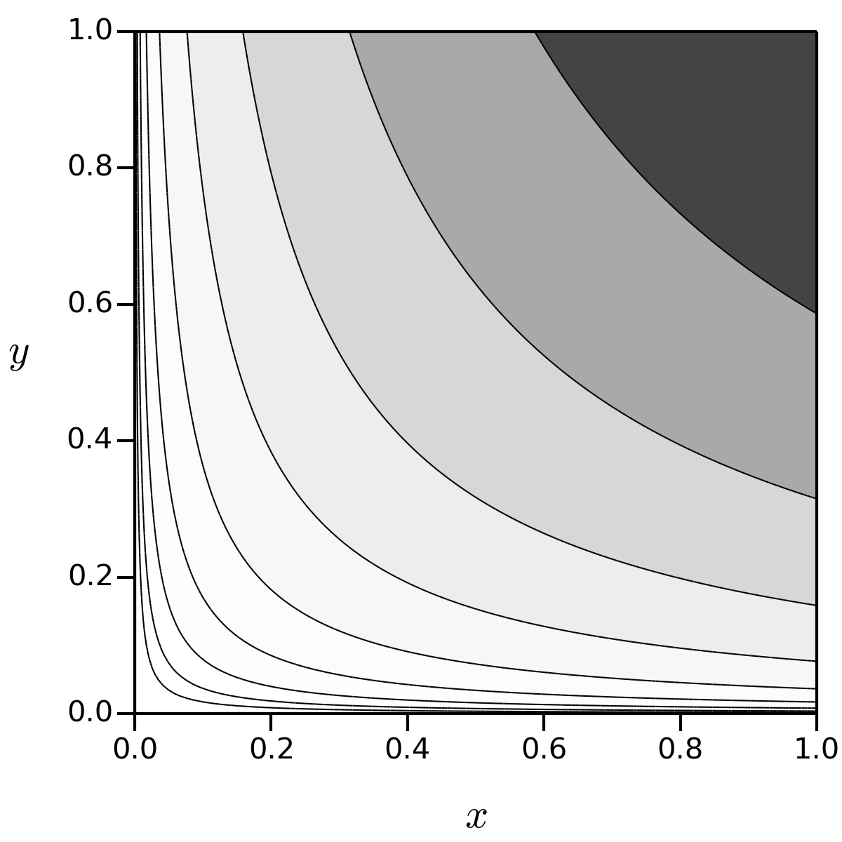
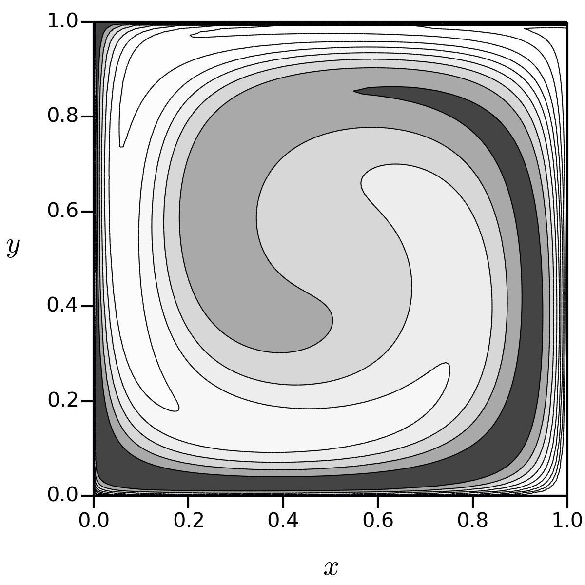
The initial condition is given by $\mathcal{U}(x,y,0)=\exp(xy)$ , and the solution is advanced for 10 nondimensional time units on a uniform grid with $N=12$ edges in each direction, i.e. there are $2N^{2}=288$ elements in total. As before, the time step is set such that the Courant number is one half the value of $\mathsf{CFL}_{\max}$ listed in Table 2; however, we emphasize that we are only interested in assessing the stability of the methods with this experiment, and the discrete solutions after 10 time units are not accurate for the coarse grids considered. To give some indication of the solution behavior and the time duration, Figure 6 shows the initial solution and the exact solution after only one unit of time.

To demonstrate that the SBP-SAT discretizations are energy stable, Figure 7 shows the change in normalized energy as the discrete solutions evolve from $t=0$ to $t=10$ . The normalized change in energy is given by

\frac{\bm{u}(t)^{T}\mathsf{H}_{g}\bm{u}(t)-\bm{u}_{0}^{T}\mathsf{H}_{g}\bm{u}_{0}}{\bm{u}_{0}^{T}\mathsf{H}_{g}\bm{u}_{0}}=\frac{\|\bm{u}(t)\|_{\mathsf{H}_{g}}^{2}}{\|\bm{u}_{0}\|_{\mathsf{H}_{g}}^{2}}-1

where $\bm{u}(t)$ denotes the discrete solution at time $t$ . As with the conservation metric, we consider a uniform triangulation with $N=12$ edges in each direction and 288 elements total.

Figures 7(a) and 7(b) show the change in energy for the SBP- $\Gamma$ and SBP- $\Omega$ families applied to the skew-symmetric discretization (18) with upwind SATs. The plots show that the SBP-SAT discretizations have nonincreasing energies, as expected from the analysis in Sections 4 and 5.2. In contrast, Figure 7(c) shows the change in energy for the SBP- $\Gamma$ family applied to the “divergence” form of the discretization, namely

\frac{d\mathsf{J}\bm{u}}{dt}+\mathsf{D}_{\xi}\Lambda_{\xi}\bm{u}+\mathsf{D}_{\eta}\Lambda_{\eta}\bm{u}=\bm{\mathrm{SAT}}_{\bm{u}}.

As the plots show, only the skew-symmetric discretizations have bounded energies³³ 3 For this problem the discretization of the divergence form leads to increasing energy, but this is not always the case. Indeed, when solving the constant-coefficient, curvilinear-coordinate problem we did not encounter increasing energy.

8 Conclusions

Multi-dimensional SBP operators offer time-stable, high-order, and conservative discretizations on complex domains, but only if boundary conditions and inter-element coupling can be imposed in a suitable manner. To this end, we have proposed a general framework for the development of SATs that lead to accurate, stable, and conservative schemes. We focused on developing a set of SATs that are simple to construct and that allow for the pointwise imposition of boundary conditions and inter-element coupling. This was accomplished by using interpolation/extrapolation operators and face-based cubatures to construct the coupling terms in the SATs. A key insight of this paper is that the $\mathsf{E}$ matrices and the coupling terms in the SATs can be decomposed in the same way; this insight significantly simplifies the development of this class of SATs.

Using these SATs, we showed how to derive conservative and time-stable discretizations for multi-dimensional SBP operators in the context of the linear advection equation with a spatially varying velocity field. In this context, conservation requires a particular relationship between the interpolated/extrapolated fluxes and the SATs. For a divergence-free problem, we satisfied this conservation condition by projecting the analytical advection field onto a field that satisfies a discrete form of the divergence-free equation. For nonlinear hyperbolic systems of PDEs, numerical flux functions can be used to satisfy the conservation condition.

The SAT methodology was illustrated using SBP operators on triangular elements. Two SBP families were considered: the SBP- $\Gamma$ family with $p+1$ nodes on each face and the SBP- $\Omega$ family with strictly interior nodes.

The accuracy, conservation, and stability properties of the SBP-SAT discretizations were verified using the linear advection equation with divergence-free velocity fields. Both the SBP- $\Omega$ and SBP- $\Gamma$ schemes were shown to be conservative to machine precision, and both produced non-increasing energy. For the same operator degree $p$ , the SBP- $\Omega$ scheme was found to be more accurate. Finally, we numerically demonstrated that the SBP-SAT discretizations presented result in superconvergent functional estimates.

Appendix A Satisfaction of the discrete divergence-free equation

In general, the analytical velocity, which we will denote here as $\hat{\bm{\lambda}}_{\xi}$ , does not satisfy the discretized divergence-free condition, (28). Therefore, we seek a discrete vector field that satisfies the discrete divergence-free condition and is as close as possible, in some norm, to the analytical field. This appendix describes how find such a discrete vector field.

First we solve for the face-normal velocities, $(\lambda_{n})_{i}=\left(\lambda_{\xi}n_{\xi}+\lambda_{\eta}n_{\eta}\right)_{i}$ , that appear in the elements of the $\mathsf{B}_{\lambda}$ matrices. A constraint on the $(\lambda_{n})_{i}$ for each element is obtained by substituting $\bm{v}=\bm{1}$ into the identity (29):

\sum_{j=1}^{\kappa}\left(\bm{1}_{\hat{\Gamma}_{j}}^{\mathrm{T}}\mathsf{B}_{\lambda,j}\mathsf{R}_{j}\right)\bm{1}=\sum_{j=1}^{\kappa}\sum_{i=1}^{n_{j}}b_{i}^{(j)}\left(\lambda_{n}^{(j)}\right)_{i}=\bm{1}^{T}\left(\Lambda_{\xi}\mathsf{Q}_{\xi}+\Lambda_{\eta}\mathsf{Q}_{\eta}\right)\bm{1}=0,

where the last equality follows from $\mathsf{Q}_{\xi}\bm{1}=\mathsf{Q}_{\eta}\bm{1}=\bm{0}$ . This constraint is simply a discretization of $\int_{\hat{\Gamma}}\bm{\lambda}\cdot\bm{n}\,\mathrm{d}\hat{\Gamma}=0$ on each element. There are fewer elements than face-normal velocities, so we solve a quadratic optimization problem that minimizes the Cartesian norm between the discrete and analytical values at the face nodes, $(\lambda_{n}^{(j)})_{i}$ and $(\hat{\lambda}_{n}^{(j)})_{i}$ , respectively, subject to the above constraint.

Once the $\mathsf{B}_{\lambda}$ matrices are determined, we solve for the diagonal matrices $\Lambda_{\xi}$ and $\Lambda_{\eta}$ . We follow a procedure analogous to the one used for $\mathsf{B}_{\lambda}$ ; in this case we minimize the Cartesian norm between the discrete and analytical values at the SBP nodes and (28) becomes the constraint. The optimization problems on each element are decoupled.

For the cases considered here, we verified that the $L^{2}$ error in the discrete velocity field is at least an order of magnitude smaller than the $L^{2}$ error in the scalar field $\mathcal{U}$ . Moreover, the error in the velocity field decreases with $h$ , the average mesh spacing, at a faster rate than the error in $\bm{u}$ , and the error in the velocity field has an insignificant impact on the solution error.

References

(1) Parsani, M., Carpenter, M. H., and Nielsen, E. J., “Entropy stable wall boundary conditions for the three-dimensional compressible Navier-Stokes equations,” Journal of Computational Physics, Vol. 292, No. C, 2015, pp. 88–113.
(2) Carpenter, M. H., Fisher, T. C., Nielsen, E. J., and Frankel, S. H., “Entropy Stable Spectral Collocation Schemes for the Navier–Stokes Equations: Discontinuous Interfaces,” SIAM Journal on Scientific Computing, Vol. 36, No. 5, 2014, pp. B835–B867.
(3) Fisher, T. C. and Carpenter, M. H., “High-order entropy stable finite difference schemes for nonlinear conservation laws: Finite domains,” Journal of Computational Physics, Vol. 252, No. 1, 2013, pp. 518–557.
(4) Kreiss, H.-O. and Scherer, G., “Finite element and finite difference methods for hyperbolic partial differential equations,” Mathematical aspects of finite elements in partial differential equations, Academic Press, New York/London, 1974, pp. 195–212.
(5) Strand, B., “Summation by parts for finite difference approximations for d/dx,” Journal of Computational Physics, Vol. 110, No. 1, 1994, pp. 47–67.
(6) Del Rey Fernández, D. C., Hicken, J. E., and Zingg, D. W., “Review of summation-by-parts operators with simultaneous approximation terms for the numerical solution of partial differential equations,” Computers & Fluids, Vol. 95, No. 22, 2014, pp. 171–196.
(7) Svärd, M. and Nordström, J., “Review of summation-by-parts schemes for initial-boundary-value-problems,” Journal of Computational Physics, Vol. 268, No. 1, 2014, pp. 17–38.
(8) Del Rey Fernández, D. C. and Zingg, D. W., “Generalized summation-by-parts operators for the second derivative with a variable coefficient,” SIAM Journal on Scientific Computing, Vol. 37, No. 6, 2015, pp. A2840–A2864.
(9) Del Rey Fernández, D. C., Boom, P. D., and Zingg, D. W., “A Generalized Framework for Nodal First Derivative Summation-By-Parts Operators,” Journal of Computational Physics, Vol. 266, No. 1, 2014, pp. 214–239.
(10) Gassner, G. J., “A skew-symmetric discontinuous Galerkin spectral element discretization and its relation to SBP-SAT finite difference methods,” SIAM Journal on Scientific Computing, Vol. 35, No. 3, 2013, pp. A1233–A1253.
(11) Carpenter, M. H. and Gottlieb, D., “Spectral methods on arbitrary grids,” Journal of Computational Physics, Vol. 129, No. 1, 1996, pp. 74–86.
(12) Nordström, J., Forsberg, K., Adamsson, C., and Eliasson, P., “Finite volume methods, unstructured meshes and strict stability for hyperbolic problems,” Applied Numerical Mathematics, Vol. 45, 2003, pp. 453–473.
(13) Hicken, J. E., Del Rey Fernández, D. C., and Zingg, D. W., “Multi-dimensional Summation-By-Parts Operators: General Theory and Application to Simplex Elements,” SIAM Journal on Scientific Computing, Vol. 38, No. 4, 2016, pp. A1935–A1958.
(14) Hicken, J. E., Del Rey Fernández, D. C., and Zingg, D. W., “Opportunities for efficient high-order methods based on the summation-by-parts property,” 22nd AIAA Computational Fluid Dynamics Conference, No. AIAA–2015–3198, Dallas, Texas, June 2015.
(15) Cools, R., “Monomial cubature rules since “Stroud”: a compilation — part 2,” Journal of Computational and Applied Mathematics, Vol. 112, No. 1–2, 1999, pp. 21 – 27.
(16) Carpenter, M. H., Gottlieb, D., and Abarbanel, S., “Time-stable boundary conditions for finite-difference schemes solving hyperbolic systems: Methodology and application to high-order compact schemes,” Journal of Computational Physics, Vol. 111, No. 2, 1994, pp. 220–236.
(17) Carpenter, M. H., Nordström, J., and Gottlieb, D., “A stable and conservative interface treatment of arbitrary spatial accuracy,” Journal of Computational Physics, Vol. 148, No. 2, 1999, pp. 341–365.
(18) Nordström, J. and Carpenter, M. H., “Boundary and interface conditions for high-order finite-difference methods applied to the Euler and Navier-Stokes equations,” Journal of Computational Physics, Vol. 148, No. 2, 1999, pp. 621–645.
(19) Nordström, J. and Carpenter, M. H., “High-order finite-difference methods, multidimensional linear problems, and curvilinear coordinates,” Journal of Computational Physics, Vol. 173, No. 1, 2001, pp. 149–174.
(20) Hesthaven, J. S. and Warburton, T., Nodal discontinuous Galerkin methods: algorithms, analysis, and applications, Springer-Verlag, New York, 2008.
(21) Harten, A., “On the symmetric form of systems of conservation laws with entropy,” Journal of Computational Physics, Vol. 49, No. 1, 1983, pp. 151–164.
(22) Hughes, T. J. R., Franca, L. P., and Mallet, M., “A new finite element formulation for computational fluid dynamics: I. symmetric forms of the compressible Navier-Stokes equations and the second law of thermodymaics,” Computer Methods in Applie Mechanics and Engineering, Vol. 54, No. 2, April 1986, pp. 223–234.
(23) Gassner, G. J., Winters, A. R., and Kopriva, D. A., “Split form nodal discontinuous Galerkin schemes with summation-by-parts property for the compressible Euler equations,” arXiv:1604.06618v2 [math.NA], 2016, pp. 28–50.
(24) Kopriva, D. A. and Gassner, G. J., “An energy stable discontinuous Galerkin spectral element discretization for variable coefficient advection problems,” SIAM Journal on Scientific Computing, Vol. 4, No. 36, 2014, pp. A2076–A2099.
(25) Gustafsson, B., Kreiss, H.-O., and Oliger, J., Time-Dependent Problems and Difference Methods, Pure and Applied Mathematics, Wiley, 2nd ed., 2013.
(26) Kreiss, H.-O. and Lorenz, J., Initial-Boundary Value Problems and the Navier-Stokes Equations, Vol. 47 of Classics in Applied Mathematics, SIAM, 2004.
(27) Thomas, P. D. and Lombard, C. K., “Geometric conservation law and its application to flow computations on moving grids,” AIAA Journal, Vol. 17, No. 10, Oct. 1979, pp. 1030–1037.
(28) Hicken, J. E. and Zingg, D. W., “Superconvergent functional estimates from summation-by-parts finite-difference discretizations,” SIAM Journal on Scientific Computing, Vol. 33, No. 2, 2011, pp. 893–922.

Simultaneous Approximation Terms for Multi-Dimensional Summation-by-Parts Operators

Abstract

1 Introduction

2 Notation and review of multi-dimensional summation-by-parts operators

Definition 1

3 Decomposition of 𝖤ξ\mathsf{E}_{\xi}

Assumption 1

Remark 1

Theorem 1

Proof

Theorem 2

Proof

Corollary 1

Remark 2

4 Linear variable-coefficient PDEs

4.1 Stability and conservation of the variable-coefficient linear advection equation

Remark 3

4.2 The generic SBP-SAT semi-discretization

4.2.1 Stability

Condition 1 (Stability)

4.2.2 Accuracy

Condition 2 (Accuracy)

4.2.3 Conservation

Condition 3 (Conservation)

4.3 Divergence-free advection field

Condition 3′ (Divergence-Free Conservation)

5 Concrete examples of SATs: symmetric and upwind SATs

Assumption 2

Remark 4

Remark 5

Remark 6

5.1 Symmetric SATs

Theorem 3

Proof

5.2 Upwind SATs

Theorem 4

Proof

5.3 Divergence-free advection field with upwind SATs

Remark 7

6 Example operators on the triangle

7 Numerical verifications

7.1 Constant-coefficient advection with a curvilinear coordinate mapping

7.1.1 Accuracy

7.1.2 Conservation

7.1.3 Stability

Remark 8

7.2 Robustness of SBP-SAT discretizations: advection in a confined domain

8 Conclusions

Appendix A Satisfaction of the discrete divergence-free equation

References

3 Decomposition of $\mathsf{E}_{\xi}$

Condition 3^′ (Divergence-Free Conservation)