A possible interpretation of the Higgs mass by the cosmological attractive relaxion

Recently, a novel type of resolution for the electroweak (EW) hierarchy problem ¹¹ 1 Many mechanisms have been proposed to solve the EW hierarchy problem, including the extra dimensions theory, the supersymmetry theory, and the compositeness of the Higgs boson [3, 4, 5, 6, 7]. However, all these new models lead to a technically natural EW scale [40], since the current experimental data from the colliders and indirect experiments have put their model parameters into fine-tuned regions. Or, we can just ignore the EW hierarchy problem if we believe the anthropic principle. has been proposed (relaxion mechanism) in Ref. [2], which is very different from the traditional approaches (either weak scale dynamics [3, 4, 5, 6, 7] or anthropics). In this relaxion mechanism, the relevant fields below the cutoff scale are just the standard model (SM) fields plus the axion field with unspecified inflation sector being involved, and the Higgs mass is dependent on the axion field [2], which is motivated from Abbott’s field-dependent idea to solve the cosmological constant problem [8]. Accordingly, the cosmological evolution of the Higgs mass and the specific axion potential choose the EW scale, which is smaller than the cutoff of the theory. The highest cutoff relaxed in Ref. [2] is about $10^{8}$ GeV. This relaxion mechanism can technically relax the EW hierarchy problem and has become a theoretical highlight in frontier studies of the hierarchy problem and exploring new physics beyond the SM [9, 10, 11, 12, 13, 14, 15, 16, 17, 18, 19, 20, 21, 22, 23, 24, 25]. Especially, this new mechanism opens a new window to understand some puzzles and key parameters in particle physics from the aspect of cosmological evolution.

Following this cosmological evolution idea, our toy model here takes advantage of the attractive properties of the “$\alpha$-attractors” [26, 27, 28, 29, 30, 31, 32, 33, 34, 35, 36, 37, 38] to fix the Higgs mass at today’s value rather than the increasing potential barriers of the axion potential in  [2]. In recent years, Linde and Kallosh have proposed a broad class of supergravity inflationary models based on conformal symmetry in the Jordan frame, where a universal attractor behavior exists in the Einstein frame [26, 27, 28, 29, 30, 31, 32, 33, 34, 35, 36, 37, 38]. These classes of supergravity inflationary models are called “$\alpha$-attractors”, since their potentials involve a free parameter $\alpha$ [31, 32, 33, 34, 35, 36, 37, 38]. These inflation models of “$\alpha$-attractors” mainly have two classes: one is the so-called T-models with the potential $f^{2}(\tanh(\phi/(\sqrt{6\alpha}\rm M_{\rm pl})))$ and the other is the so-called E-models with the potential $f^{2}(1-\exp(-\sqrt{2/3\alpha}\phi/\rm M_{\rm pl}))$ in the Einstein frame. In the limits of small $\alpha$ and large $e$-folding number $\text{N}_{e}$, these models have the same predictions [31, 32, 33, 34, 35, 36, 37, 38] corresponding to the central area of the $n_{\textrm{s}}-r$ plane favored by the data of Planck 2015 [39].

Our toy model here only tries to provide a possible cosmological interpretation of the light Higgs mass, and only the attractive inflation field is needed motivated from the above relaxion mechanism and the attractive inflation. Here, we do not consider the UV-completed theory for a fully natural theory. In addition, our models may be tested in particle physics experiments.

In Section 2, we first describe the cosmological scenario to explain the light mass of the Higgs boson by attractive inflation. In Section 3, we study the possible signals or constraints in future lepton colliders and the constraints from the muon anomalous magnetic moment. Then, in Section 4, we perform a detailed analysis of cosmological perturbations seeded by the inflation fields in a concrete model. Section 5 gives a brief summary.

In this section, we show a possible cosmological scenario to explain the light mass of the Higgs boson by attractive inflation. In our toy model, the field contents below the cutoff scale are just the SM fields and the inflaton field. The relevant potential can be written as

$$V(\phi,h)=\frac{\lambda_{SM}}{4}h^{4}+\frac{(g^{2}\phi^{2}-\text{M}^{2})}{2}h^{2}+V_{att},$$

(1)

where the field $h$ and $\rm\phi$ represent the Higgs field and the inflaton field, respectively. The second term in Eq.(1) generally can be the form of $(f(\phi)-\text{M}^{2})h^{2}/2$. In this scenario, the Higgs mass in the early universe is field dependent, namely, $m_{h}^{2}=g^{2}\phi^{2}-\rm M^{2}$. This is just the starting point of our discussion. We assume that the initial value of the inflation field $\phi$ starts at $\phi\gg\text{M}/g$, where M represents the cutoff scale in this toy model. Thus, the mass of the Higgs boson in the early universe is naturally set to be the order of the cutoff scale M. Here, $V_{att}$ means the attractive potential, which can drive the cosmological inflation and fix the current Higgs mass. Interestingly, the potentials in a broad class of supergravity inflation models (the so-called “$\alpha$-attractors”) [31, 32, 33, 34, 35, 36, 37, 38] can just satisfy the requirements. One class of potentials is given by [31, 32, 33, 34, 35, 36, 37, 38]

$$V_{att}=V_{\text{T}}=\text{M}^{4}\tanh^{2\text{T}}\biggl({\phi-\phi_{c}\over\sqrt{6\alpha}{\rm M_{\rm pl}}}\biggr),$$

(2)

where $\text{M}_{\rm pl}$ is the reduced Planck mass. This class of potential is just the potential in the T-models of “$\alpha$-attractors”. The potential $V_{\text{T}}$ can be obtained from canonical Kahler potential such as $(\Phi-\bar{\Phi})^{2}$ in the supergravity model. The non-minimal coupling case between the inflaton field and the gravitational field can also lead to the same predictions when compared to this type of attractive potential in some limits. The other type of attractive potential can be written as [31, 32, 33, 34, 35, 36, 37, 38]

$$V_{att}=V_{\text{E}}=\text{M}^{4}\left(1-e^{-{\sqrt{2\over 3\alpha}}(\phi-\phi_{c})/\text{M}_{\rm pl}}\right)^{2\text{E}}\ .$$

(3)

This potential can be motivated by considering a vector rather than a chiral multiplet for the inflation models in supergravity, and is just the potential in the so-called E-model. Here, the power exponents T and E in Eqs. (2) and (3) are integers and $\alpha$ is the free parameters. $\phi_{c}$ is a constant, which is related to the current Higgs boson mass.

We take the potential $V_{\text{T}}$ as an example to illuminate the cosmological origin of the light Higgs boson mass. Firstly, under the slow-roll approximation, the spectral index $n_{s}$, the tensor-to-scalar ratio $r$, and the e-folding number $\text{N}_{e}$ as functions of $\phi$ can be obtained:

	$\displaystyle n_{s}=1-{1\over 3\alpha}\biggl[4T~{\rm sech}^{2}{\sqrt{1\over 6\alpha}{\phi-\phi_{c}\over\text{M}_{\rm pl}}}$
	$\displaystyle+8\text{T}(1+\text{T})~{\rm csch}^{2}{\sqrt{2\over 3\alpha}{\phi-\phi_{c}\over\text{M}_{\rm pl}}}\biggr],$
	$\displaystyle r={64\text{T}^{2}~{\rm csch}^{2}{\sqrt{2\over 3\alpha}{\phi-\phi_{c}\over\text{M}_{\rm pl}}}\over 3\alpha},$
	$\displaystyle\text{N}_{e}=-{3\alpha\over 4\text{T}}\biggl[\cosh{\sqrt{2\over 3\alpha}{\phi_{\rm end}-\phi_{c}\over\text{M}_{\rm pl}}}-\cosh{\sqrt{2\over 3\alpha}{\phi-\phi_{c}\over\text{M}_{\rm pl}}}\biggr].$

For the E-models, the corresponding results are

	$\displaystyle n_{s}$	$\displaystyle=$	$\displaystyle 1-\frac{8\text{E}(\text{E}+e^{\sqrt{\frac{2}{3\alpha}}\frac{\phi-\phi_{c}}{\text{M}_{\rm pl}}})}{3\alpha(-1+e^{\sqrt{\frac{2}{3\alpha}}\frac{\phi-\phi_{c}}{\text{M}_{\rm pl}}})^{2}},$
	$\displaystyle r$	$\displaystyle=$	$\displaystyle\frac{64\text{E}^{2}}{3\alpha(-1+e^{\sqrt{\frac{2}{3\alpha}}\frac{\phi-\phi_{c}}{\text{M}_{\rm pl}}})^{2}},$
	$\displaystyle\text{N}_{e}$	$\displaystyle=$	$\displaystyle-\frac{3\alpha}{4\text{E}}\biggl[e^{\sqrt{\frac{2}{3\alpha}}\frac{\phi_{end}-\phi_{c}}{\text{M}_{\rm pl}}}-e^{\sqrt{\frac{2}{3\alpha}}\frac{\phi-\phi_{c}}{\text{M}_{\rm pl}}}+\sqrt{\frac{2}{3\alpha}}\frac{\phi-\phi_{end}}{\text{M}_{\rm pl}}\biggr].$

These types of potential in the small $\alpha$ limit are favored by the data from Planck 2015 [39].

Firstly, in the very early universe $\phi\gg\text{M}/g$, the effective mass-squared of the Higgs boson $m_{h}^{2}$ is positive and the vacuum expectation value (vev) of the Higgs field is zero. The final solution is insensitive to the initial condition of $\phi$ as long as the initial mass-squared of the Higgs $m_{h}^{2}$ is positive, since it is slow-rolling due to Hubble friction. The inflaton field $\phi$ drives the slow-roll inflation by the attractive potential $V_{att}=V_{\text{T}}=\text{M}^{4}\tanh^{2\text{T}}\biggl({\phi-\phi_{c}\over\sqrt{6\alpha}{\rm M_{\rm pl}}}\biggr)$ or $V_{att}=V_{\text{E}}=\text{M}^{4}\left(1-e^{-{\sqrt{2\over 3\alpha}}(\phi-\phi_{c})/\text{M}_{\rm pl}}\right)^{2\text{E}}$ as shown in Fig. 1. With the evolution of the universe, the inflaton field naturally crosses the critical point for the Higgs mass where $m_{h}^{2}=0$, namely, a transition point occurs when $\phi=\text{M}/g$. When the inflaton field across this critical point with $\phi<\text{M}/g$, the mass-squared term $m_{h}^{2}$ transits from a positive value to a negative value, and then the Higgs field acquires a vev. Thereby, the cosmological inflation can scan the physical mass of the Higgs boson, as shown in Fig. 1.

After reheating and dissipation²² 2 After the inflation ends, the reheating process may be important in these models [41], but we leave this for future work., the inflaton field $\phi$ is stuck in the vicinity of $\phi_{c}$. Thus, the Higgs mass evolves from a large field-dependent mass to the currrent $125$ GeV mass. In the early universe, the field dependent mass of the Higgs boson is $m_{h}^{2}=g^{2}\phi^{2}(t)-\text{M}^{2}$, where $\phi(t)\gg\phi_{e}$. During the cosmological evolution, the mass of the Higgs boson becomes much smaller. When the inflaton is stuck by the attractive potential of $\phi$ as shown in Fig. 1, the Higgs mass is fixed as $\mu^{2}=g^{2}\phi_{c}^{2}-\text{M}^{2}<0$. Here, $\mu^{2}$ is the coefficient of the $h^{2}$ in the SM with $m_{h}^{2}=-2\mu^{2}=(\rm 125GeV)^{2}$. This provides a cosmological interpretation of the light Higgs mass, and $\phi_{c}=\sqrt{\text{M}^{2}+\mu^{2}}/{g}$. For $\rm M=10^{6}$ GeV, $g=10^{-2}$, $\phi_{c}\approx 10^{8}$ GeV. We call the inflaton field $\phi$ the attractive relaxion, which has the above attractive inflation behavior.

In this section, we discuss the possible collider signals or constraints from particle physics experiments for two simple cases of Higgs portal interactions $f(\phi)h^{2}/2$.

In this section, we study a concrete attractive relaxion model, assuming a non-minimal coupling of the inflation field $\phi$ to gravity, namely $(1/2)\xi R\phi^{2}$ [44]. Such a non-minimal coupling may arise from some quantum gravity effects, such as the Higgs field with asymptotically safe gravity [45, 46]. We begin the discussion with the following action [44] in the Jordan frame:

	$\displaystyle S=\int d^{4}x\sqrt{-\hat{g}}(\frac{1-\xi\kappa^{2}(\phi-\phi_{c})^{2}}{2\kappa^{2}}R(\hat{g})$
	$\displaystyle-\frac{1}{2}(\hat{\nabla}\phi)^{2}-\frac{1}{2}(\hat{\nabla}h)^{2}-V(\phi,h),$		(8)

where

$$V(\phi,h)=\frac{\lambda_{SM}}{4}h^{4}+\frac{(g^{2}\phi^{2}-\text{M}^{2})}{2}h^{2}+\frac{\lambda}{4}(\phi-\phi_{c})^{4},$$

(9)

and $\kappa^{2}/8\pi=\text{G}$, which G is Newton’s gravitational constant.

Performing the Weyl conformal transformation with $\Omega^{2}=1-\xi\kappa^{2}(\phi-\phi_{c})^{2}$ and defining a new field $\varphi_{1}$ to make the kinetic term of $\phi$ be canonical as

$\displaystyle\varphi_{1}=\int\sqrt{\frac{1-(1-6\xi)\xi\kappa^{2}(\phi-\phi_{c})^{2}}{(1-\xi\kappa^{2}(\phi-\phi_{c})^{2})^{2}}}d\phi,$

(10)

or

$\displaystyle\frac{d\varphi_{1}}{d\phi}=\sqrt{\frac{1-(1-6\xi)\xi\kappa^{2}(\phi-\phi_{c})^{2}}{(1-\xi\kappa^{2}(\phi-\phi_{c})^{2})^{2}}},$

(11)

we obtain the following action in the Einstein frame:

	$\displaystyle S=\int d^{4}x\sqrt{-g}(\frac{1}{2\kappa^{2}}R-\frac{1}{2}(\nabla\varphi_{1})^{2}$
	$\displaystyle-\frac{1}{2}e^{-2F(\varphi_{1})}(\nabla h)^{2}-U(\varphi_{1},h)),$		(12)

with

	$\displaystyle F=\frac{1}{2}\ln|1-\xi\kappa^{2}(\phi-\phi_{c})^{2}|,$
	$\displaystyle U=e^{-4F(\varphi_{1})}V=\frac{V}{(1-\xi\kappa^{2}(\phi-\phi_{c})^{2})^{2}}.$

We use the longitudinal gauge (Newton gauge),

$$ds^{2}=-(1+2\Phi)dt^{2}+a^{2}(t)(1-2\Psi)\delta_{ij}dx^{i}dx^{j},$$

(13)

and take $\Phi=\Psi$ here.

Firstly, we derive the background field evolution equations for the cosmic expansion rate $H=\dot{a}/a$ and homogeneous parts of scalar fields by variation of the action in Eq.(12) :

$\displaystyle H^{2}=\frac{\kappa^{2}}{3}\left(\frac{1}{2}\dot{\varphi}_{1}^{2}+\frac{1}{2}e^{-2F}\dot{h}^{2}+U\right),$

(14)

$\displaystyle\dot{H}=-\frac{\kappa^{2}}{2}\left(\dot{\varphi}_{1}^{2}+e^{-2F}\dot{h}^{2}\right),$

(15)

$\displaystyle\ddot{\varphi}_{1}+3H\dot{\varphi}_{1}+U_{,\varphi_{1}}+F_{,\varphi_{1}}e^{-2F}\dot{h}^{2}=0,$

(16)

$\displaystyle\ddot{h}+3H\dot{h}+e^{2F}U_{,h}-2F_{,\varphi_{1}}\dot{\varphi}_{1}\dot{h}=0,$

(17)

Secondly, following the standard perturbative methods in cosmological inflation [47], we obtain the Fourier-transformed, first-order Einstein equations for the metric and field fluctuations as

	$\displaystyle\ddot{\Phi}+4H\dot{\Phi}+\kappa^{2}U\Phi$
	$\displaystyle=\frac{\kappa^{2}}{2}\left[\dot{\varphi}_{1}\delta\dot{\varphi}_{1}-(U_{,\varphi_{1}}+F_{,\varphi_{1}}e^{-2F}\dot{h}^{2})\delta\varphi_{1}+e^{-2F}\dot{h}\delta\dot{h}-U_{,h}\delta h\right],$

	$\displaystyle-\frac{\kappa^{2}}{2}(\dot{\varphi}_{1}\delta\dot{\varphi}_{1}+(3H\dot{\varphi}_{1}+U_{,\varphi_{1}}-F_{,\varphi_{1}}e^{-2F}\dot{h}^{2})\delta\varphi_{1}$
	$\displaystyle+e^{-2F}\dot{h}\delta\dot{h}+(U_{,h}+3H\dot{h}e^{-2F})\delta h)$
	$\displaystyle=\left(\frac{k^{2}}{a^{2}}-\dot{H}\right)\Phi,$

$\displaystyle\dot{\Phi}+H\Phi=\frac{\kappa^{2}}{2}\left(\dot{\varphi}_{1}\delta\varphi_{1}+e^{-2F}\dot{h}\delta h\right),$

			$\displaystyle\delta\ddot{\varphi}_{1}+3H\delta\dot{\varphi}_{1}+\left[\frac{k^{2}}{a^{2}}+U_{,\varphi_{1}\varphi_{1}}-\left(e^{-2F}\right)_{,\varphi_{1}\varphi_{1}}\frac{\dot{h}^{2}}{2}\right]\delta\varphi_{1}$
		$\displaystyle=$	$\displaystyle 4\dot{\varphi}_{1}\dot{\Phi}-2U_{,\varphi_{1}}\Phi-2F_{,\varphi_{1}}e^{-2F}\dot{h}\delta\dot{h}+U_{,\varphi_{1}h}\delta h,$

	$\displaystyle\delta\ddot{h}+(3H-2F_{,\varphi_{1}}\dot{\varphi}_{1})\delta\dot{h}+\left(\frac{k^{2}}{a^{2}}+e^{2F}U_{,hh}\right)\delta h-2F_{,\varphi_{1}}\dot{h}\delta\dot{\varphi}_{1}$
	$\displaystyle=4\dot{h}\dot{\Phi}-2e^{2F}U_{,h}\Phi-e^{2F}\left(2F_{,\varphi_{1}}U_{,h}+U_{,\varphi_{1}h}-2F_{,\varphi_{1}\varphi_{1}}\dot{\varphi_{1}}\dot{h}\right)\delta\varphi_{1}.$

For $\xi>0$, $F=\frac{1}{2}\ln(1-\xi\kappa^{2}(\phi-\phi_{c})^{2})$, then $e^{2F}=1-\xi\kappa^{2}(\phi-\phi_{c})^{2}$, $e^{-2F}=1/(1-\xi\kappa^{2}(\phi-\phi_{c})^{2})$, $F_{,\varphi_{1}}=F_{,\phi}/(d\varphi_{1}/d\phi)$, and $U_{,\varphi_{1}}=U_{,\phi}/(d\varphi_{1}/d\phi)$. Note that we should be careful in dealing with the original field $\phi$ and the new field $\varphi_{1}$.

Write

$$ds^{2}=a^{2}(t)[-d\tau^{2}+(\delta_{ij}+2B_{ij})dx^{i}dx^{j}],$$

(18)

then we have

$$\ddot{B}+3H\dot{B}+\frac{k^{2}}{a^{2}}B=0.$$

(19)

Setting $\text{M}_{\rm pl}=1$, then the tensor power spectrum is obtained as

$$P_{T}=\frac{4k^{3}}{\pi^{2}}B^{2},$$

(20)

and the scalar power spectrum is

$$P_{S}=\frac{k^{3}}{2\pi^{2}}\zeta^{2},$$

(21)

where the so-called Bardeen parameter is defined by

$$\zeta=\Phi-\frac{H^{2}}{\dot{H}}(\Phi+\frac{\dot{\Phi}}{H}).$$

(22)

Here, we take the single field slow-roll approximation. Then, the detailed conditions of the cosmological inflation are described by the following slow-roll parameters:

	$\displaystyle\epsilon$	$\displaystyle=\frac{1}{2}\left(\frac{dU/d{\varphi_{1}}}{U}\right)^{2},$		(23)
	$\displaystyle\eta$	$\displaystyle=\frac{d^{2}U/d{\varphi_{1}}^{2}}{U},$		(24)

where $\epsilon$ and $\eta$ represent the first and second derivatives of the inflation potential in the Einstein frame, respectively. The number of $e$-foldings $\text{N}_{e}$ is given by

$\displaystyle\text{N}_{e}$

$\displaystyle=$

$\displaystyle\frac{1}{\sqrt{2}}\int_{t_{i}}^{t_{f}}Hdt$

Thus, the amplitude of density perturbations in $k$-space under the slow-roll approximation is defined by the power spectrum:

$$P_{S}(k)=A_{S}\left(\frac{k}{k^{*}}\right)^{n_{s}-1},$$

(26)

where $A_{S}$ is the scalar amplitude at some “pivot point” $k^{*}$, which is given by

$$A_{S}=\frac{U}{24\pi^{2}\epsilon}\Bigg|_{k^{*}},$$

(27)

which can be measured from cosmic microwave background radiation(CMB) experiments. At the leading level, the scalar spectral index $n_{s}$ can be written as

$$n_{s}=1-6\epsilon+2\eta\,,$$

(28)

and the corresponding tensor-to-scalar ratio $r^{*}$ is

$$r^{*}=16\epsilon\,.$$

(29)

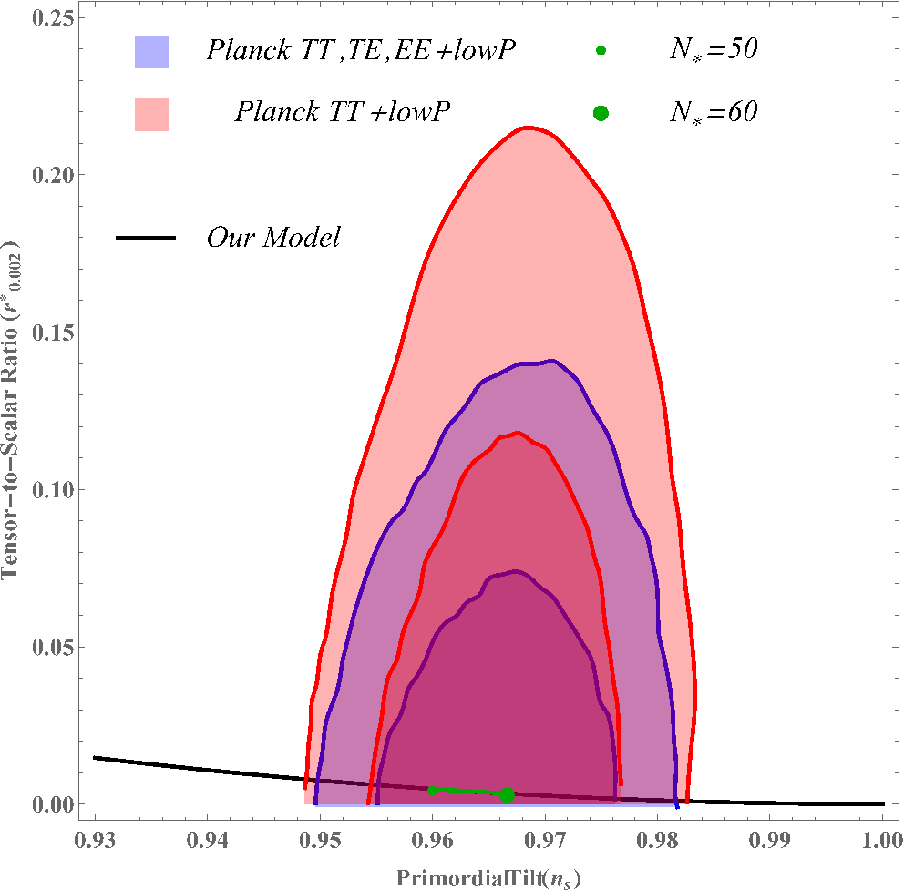
Using the recent Planck 2015 data $n_{s}=0.9655\pm 0.0062$ and $\ln(10^{10}A_{S})=3.089\pm 0.036$ [48], we can obtain the constraints on the model parameters, and fit the combined experimental results of Planck 2015 using this model in the $n_{s}-r$ plane as shown in Fig. 3, where we choose the pivot scale $k^{*}=0.002\rm{Mpc^{-1}}$, and $r_{0.002}^{*}<0.10$ at $95\%$C.L. Figure 3 shows that our prediction is well within the joint $95\%$ C.L. regions. Roughly speaking, during inflation, there may exist the effect of entropy perturbation from the Higgs field. After reheating, it can be converted to curvature perturbation if the Higgs field couples to the inflaton field. In particular, if the reheating process is realized by the so-called Higgs reheating, then this effect would be very manifest. But this only applies to the case when the coupling between the inflation field and the Higgs field is sufficiently strong. However, the coupling between them is weak in this attractive relaxion model, and thus the result for the curvature perturbation is almost unaffected³³ 3 Detailed discussions on the effects of the Higgs field are given in Ref. [46].. This non-minimal coupling model just corresponds to a special case of the T-models, which can explain the light Higgs mass from the cosmological evolution.

We have put forward a toy model, which aims at providing a possible interpretation of the Higgs mass by attractive inflation. Only the inflaton field is needed and a broad classes of inflation models with attractive potentials can satisfy the conditions. This proposal ties the puzzling light mass of the Higgs boson to an attractive inflaton field which plays an important role during cosmological evolution. The possible collider signals or constraints at the future lepton colliders, the possible constraints from the muon anomalous magnetic moment and the concrete models were also discussed in detail. The attractive relaxion idea here represents a new interplay between particle physics and cosmology, and these new ideas of cosmological evolution would open a new door to understand some key parameters of particle physics.

We thank Francis Duplessis for valuable discussions during the early work. FPH is pleased to recognize the hospitality of the Department of Astronomy when visiting at University of Science and Technology of China. FPH and XZ are supported by the NSFC (Grant Nos. 11121092, 11033005, 11375220) and by the CAS pilotB program. FPH is also supported by the China Postdoctoral Science Foundation under Grant No. 2016M590133. YFC are supported in part by the Chinese National Youth Thousand Talents Program, by the USTC start-up funding (Grant No. KY2030000049) and by the NSFC (Grant No. 11421303). HL is supported in part by the NSFC under Grant No. 11033005 and the youth innovation promotion association project and the Outstanding young scientists project of the Chinese Academy of Sciences.

References

- [2] P. W. Graham, D. E. Kaplan and S. Rajendran, Phys. Rev. Lett. 115, no. 22, 221801 (2015)
- [3] S. Dimopoulos and H. Georgi, Nucl. Phys. B 193, 150 (1981).
- [4] L. Randall and R. Sundrum, Phys. Rev. Lett. 83, 3370 (1999)
- [5] N. Arkani-Hamed, S. Dimopoulos and G. R. Dvali, Phys. Lett. B 429, 263 (1998)
- [6] L. Susskind, Phys. Rev. D 20, 2619 (1979).
- [7] S. Weinberg, Phys. Rev. D 19, 1277 (1979).
- [8] L. F. Abbott, Phys. Lett. B 150, 427 (1985).
- [9] A. Strumia, arXiv:1504.08331 [hep-ph].
- [10] J. R. Espinosa, C. Grojean, G. Panico, A. Pomarol, O. Pujol¨¤s and G. Servant, Phys. Rev. Lett. 115, no. 25, 251803 (2015)
- [11] E. Hardy, JHEP 1511, 077 (2015)
- [12] S. P. Patil and P. Schwaller, JHEP 1602, 077 (2016)
- [13] O. Antipin and M. Redi, JHEP 1512, 031 (2015)
- [14] J. Jaeckel, V. M. Mehta and L. T. Witkowski, Phys. Rev. D 93, no. 6, 063522 (2016)
- [15] R. S. Gupta, Z. Komargodski, G. Perez and L. Ubaldi, JHEP 1602, 166 (2016)
- [16] B. Batell, G. F. Giudice and M. McCullough, JHEP 1512, 162 (2015)
- [17] O. Matsedonskyi, JHEP 1601, 063 (2016)
- [18] J. Ellis, arXiv:1509.07336 [hep-ph].
- [19] L. Marzola and M. Raidal, arXiv:1510.00710 [hep-ph].
- [20] K. Choi and S. H. Im, JHEP 1601, 149 (2016)
- [21] D. E. Kaplan and R. Rattazzi, Phys. Rev. D 93, no. 8, 085007 (2016)
- [22] S. Di Chiara, K. Kannike, L. Marzola, A. Racioppi, M. Raidal and C. Spethmann, arXiv:1511.02858 [hep-ph].
- [23] N. Fonseca, L. de Lima, C. S. Machado and R. D. Matheus, arXiv:1601.07183 [hep-ph].
- [24] J. L. Evans, T. Gherghetta, N. Nagata and Z. Thomas, arXiv:1602.04812 [hep-ph].
- [25] A. Fowlie, C. Balazs, G. White, L. Marzola and M. Raidal, arXiv:1602.03889 [hep-ph].
- [26] R. Kallosh and A. Linde, JCAP 1306, 028 (2013)
- [27] R. Kallosh and A. Linde, JCAP 1306, 027 (2013)
- [28] R. Kallosh and A. Linde, JCAP 1307, 002 (2013)
- [29] S. Ferrara, R. Kallosh, A. Linde and M. Porrati, Phys. Rev. D 88, no. 8, 085038 (2013)
- [30] R. Kallosh, A. Linde and D. Roest, Phys. Rev. Lett. 112 (2014) 1, 011303
- [31] R. Kallosh, A. Linde and D. Roest, JHEP 1311, 198 (2013)
- [32] R. Kallosh, A. Linde and D. Roest, JHEP 1408, 052 (2014)
- [33] R. Kallosh, A. Linde and D. Roest, JHEP 1409, 062 (2014)
- [34] M. Galante, R. Kallosh, A. Linde and D. Roest, Phys. Rev. Lett. 114, no. 14, 141302 (2015)
- [35] R. Kallosh and A. Linde, Phys. Rev. D 91, no. 8, 083528 (2015)
- [36] A. Linde,
- [37] J. J. M. Carrasco, R. Kallosh and A. Linde,
- [38] J. J. M. Carrasco, R. Kallosh and A. Linde,
- [39] [Planck Collaboration], arXiv:1502.01589 [astro-ph.CO].
- [40] G. ’t Hooft in “Recent Developments in Gauge Theories. Proceedings, Nato Advanced Study Institute, Cargese, France, August 26 - September 8, 1979,” G. ’t Hooft, et al, ed., NATO Sci. Ser. B 59, pp.1 (1980).
- [41] Y. Ueno and K. Yamamoto, Phys. Rev. D 93, no. 8, 083524 (2016)
- [42] CEPC-SPPC Study Group, IHEP-CEPC-DR-2015-01, IHEP-TH-2015-01, HEP-EP-2015-01.
- [43] K. A. Olive et al. [Particle Data Group Collaboration], Chin. Phys. C 38, 090001 (2014).
- [44] F. P. Huang, C. S. Li, D. Y. Shao and J. Wang, Eur. Phys. J. C 74, no. 8, 2990 (2014)
- [45] Y. F. Cai and D. A. Easson, Int. J. Mod. Phys. D 21, 1250094 (2013)
- [46] Y. F. Cai, Y. C. Chang, P. Chen, D. A. Easson and T. Qiu, Phys. Rev. D 88, 083508 (2013)
- [47] V. F. Mukhanov, H. A. Feldman and R. H. Brandenberger, Phys. Rept. 215, 203 (1992).
- [48] [Planck Collaboration], arXiv:1502.02114 [astro-ph.CO].
- [49] S. Dodelson and E. Stewart, Phys. Rev. D 65, 101301 (2002) E. D. Stewart, Phys. Rev. D 65, 103508 (2002)