Oracle Based Active Set Algorithm for Scalable Elastic Net Subspace Clustering

We first introduce the concept of an oracle point.

Notice that the oracle point is unique since $\boldsymbol{c}^{*}$ is unique, and that the oracle point cannot be computed until the optimal solution $\boldsymbol{c}^{*}$ has been computed. The next result gives a critical relationship involving the oracle point that is exploited by our active-set method.

Theorem 2.1 shows that if the oracle point $\boldsymbol{\delta}$ is known, the solution $\boldsymbol{c}^{*}$ can be written out directly. Moreover, it follows from (5) and (6) that $\boldsymbol{\delta}=\textbf{0}$ if and only if $\textbf{b}=\textbf{0}$.

In Figure 1, we depict a two dimensional example of the solution to the elastic net problem (4) for different values of the tradeoff parameter $\lambda$. As expected, the solution $\boldsymbol{c}^{\ast}$ becomes denser as $\lambda$ decreases. Moreover, as predicted by Theorem 2.1, the magnitude of the coefficient $c^{*}_{j}$ is a decaying function of the angle between the corresponding dictionary atom $\boldsymbol{a}_{j}$ and the oracle point $\boldsymbol{\delta}$ (shown in red). If $\boldsymbol{a}_{j}$ is far enough from $\boldsymbol{\delta}$ such that $|\langle\boldsymbol{a}_{j},\boldsymbol{\delta}\rangle|\leq\lambda$ holds true, then the corresponding coefficient $c^{*}_{j}$ is zero. We call the region containing the nonzero coefficients the oracle region. We can formally define the oracle region by using the quantity $\mu(\cdot,\cdot)$ to denote the coherence of two vectors, i.e.,

The oracle region is composed of an antipodal pair of spherical caps of the unit ball of $I\!\!R^{D}$ that are located at the symmetric locations $\pm\boldsymbol{\delta}/\|\boldsymbol{\delta}\|_{2}$, both with an angular radius of $\theta=\arccos(\lambda/\|\boldsymbol{\delta}\|_{2})$ (see Figure 2). From the definition of the oracle region and Theorem 2.1, it follows that $c_{j}^{*}\neq 0$ if and only if $\boldsymbol{a}_{j}\in\Delta(\textbf{b},A)$. In other words, the support of the solution $\boldsymbol{c}^{*}$ are those vectors $\boldsymbol{a}_{j}$ in the oracle region.

The oracle region also captures the behavior of the solution when columns from the matrix $A$ are removed or new columns are added. This provides the key insight into designing an active-set method for solving the optimization.

The interpretation for Proposition 2.1 is that the solution $\boldsymbol{c}^{*}(\textbf{b},A)$ does not change (modulo padding with additional zeros) when new columns are added to the dictionary $A$, as long as the new columns are not inside the oracle region $\Delta(\textbf{b},A)$. From another perspective, $\boldsymbol{c}^{*}(\textbf{b},[A,A^{\prime}])$ does not change if one removes columns from the dictionary $[A,A^{\prime}]$ that are not in the oracle region $\Delta(\textbf{b},[A,A^{\prime}])$.

This result means that the solution to the elastic net problem will certainly be changed by adding new columns that lie within the oracle region to the dictionary.

In the next section, we describe an efficient algorithm for solving the elastic net problem (4) that is based on the geometric structure and concentration behavior of the solution.

Although the elastic net optimization problem [50] has been recently introduced for subspace clustering in [12, 13, 32], such prior work does not provide an efficient algorithm that can handle large-scale datasets. In fact, such prior work solves the elastic net problem using existing algorithms that require calculations involving the full data matrix $A$ (e.g., the accelerated proximal gradient (APG) [2] is used in [12] and the linearized alternating direction method (LADM) [25] is used in [32]). Here, we propose to solve the elastic net problem (4) with an active-set algorithm that is more efficient than both APG and LADM, and can handle large-scale datasets. We call our new method (see Algorithm 1) ORacle Guided Elastic Net solver, or ORGEN for short.

The basic idea behind ORGEN is to solve a sequence of reduced-scale subproblems defined by an active set that is itself determined from the oracle region. Let $T_{k}$ be the active set at iteration $k$. Then, the next active set $T_{k+1}$ is selected to contain the indices of columns that are in the oracle region $\Delta(\textbf{b},A_{T_{k}})$, where $A_{T_{k}}$ denotes the submatrix of $A$ with columns indexed by $T_{k}$. We use Figure 3 for a conceptual illustration. In Figure 3(a) we show the columns of $A$ that correspond to the active set $T_{k}$ by labeling the corresponding columns of $A_{T_{k}}$ in red. The oracle region $\Delta(\textbf{b},A_{T_{k}})$ is the union of the red arcs in Figure 3(b). Notice that at the bottom left there is one red dot that is not in $\Delta(\textbf{b},A_{T_{k}})$ and thus must not be included in $T_{k+1}$, and two blue dots that are not in $T_{k}$ but lie in the oracle region $\Delta(\textbf{b},A_{T_{k}})$ and thus must be included in $T_{k+1}$. In Figure 3(c) we illustrate $T_{k+1}$ by green dots. This iterative procedure is terminated once $T_{k+1}$ does not contain any new points, i.e., when $T_{k+1}\subseteq T_{k}$, at which time $T_{k+1}$ is the support for $\boldsymbol{c}^{*}(\textbf{b},A)$.

The next lemma helps explain why ORGEN converges.

The following convergence result holds for ORGEN.

The result follows from Lemma 2.1, because it implies that an active set can never be repeated. Since there are only finitely many distinct active sets, the algorithm must eventually terminate with $T_{k+1}\subseteq T_{k}$. The remaining part of the proof establishes that if $T_{k+1}\subseteq T_{k}$, then $\boldsymbol{c}^{*}(\textbf{b},A_{T_{k+1}})$ gives the nonzero entries of the solution.

ORGEN solves large-scale problems by solving a sequence of reduced-size problems in step 3 of Algorithm 1. If the active set $T_{k}$ is small, then step 3 is a small-scale problem that can be efficiently solved. However, there is no procedure in Algorithm 1 that explicitly controls the size of $T_{k}$. To address this concern, we propose an alternative to step 5 in which only a small number of new points—the ones most correlated with $\boldsymbol{\delta}$—are added. Specifically,

where $S_{k}$ holds the indices of the largest $n$ entries in $\{|\boldsymbol{a}_{j}^{\top}\boldsymbol{\delta}(\textbf{b},A_{T_{k}})|:j\notin T_{k},\,\boldsymbol{a}_{j}\in\Delta(\textbf{b},A_{T_{k}})\}$; ideally, $n$ should be chosen so that the size of $T_{k+1}$ is bounded by a predetermined value $N_{\max}$ that represents the maximum size subproblem that can be handled in step 3. If $N_{\max}$ is chosen large enough that the second set in the union in (9) is non-empty, then our convergence result still holds.

Our analysis is built upon the optimization problem $\min_{\boldsymbol{c}}f(\boldsymbol{c};\boldsymbol{x}_{j},X_{-j}^{\ell})$. Note that its solution is trivially subspace preserving since the dictionary $X_{-j}^{\ell}$ is contained in $\mathcal{S}_{\ell}$. We then treat all points from other subspaces as newly added columns to $X_{-j}^{\ell}$ and apply Propositions 2.1 and 2.2. We get the following geometric result.

We illustrate the geometry implied by Lemma 3.1 in Figure 4, where we assume $\mathcal{S}_{\ell}$ is a two dimensional subspace in $I\!\!R^{3}$. The dictionary $X_{-j}^{\ell}$ is represented by the blue dots in the plane and the oracle region $\Delta(\boldsymbol{x}_{j},X_{-j}^{\ell})$ is denoted as the two red circles. The green dots are all other points in the dictionary. Lemma 3.1 says that $\boldsymbol{c}^{*}(\boldsymbol{x}_{j},X_{-j})$ is subspace preserving if and only if all green dots lie outside of the red region.

To ensure that a solution is subspace preserving one desires a small oracle region, while to ensure connectedness one desires a large oracle region. These facts again highlight the trade-off between these two properties. Recall that the elastic net balances $\ell_{1}$ regularization (promotes sparse solutions) and $\ell_{2}$ regularization (promotes dense solutions). Thus, one should expect that the oracle region will decrease in size as $\lambda$ is increased from $0$ towards $1$. Theorem 3.1 formalizes this claim, but first we need the following definition that characterizes the distribution of the data in $X_{-j}^{\ell}$.

To understand the next result, we comment that the size of the oracle region $\Delta(\boldsymbol{x}_{j},X_{-j}^{\ell})$ is controlled by the quantity $\lambda/\|\boldsymbol{\delta}(\boldsymbol{x}_{j},X_{-j}^{\ell})\|_{2}$ as depicted in Figure 2.

The above theorem allows us to determine an upper bound for the size of the oracle region. This follows since a lower bound on the size of $\lambda/\|\boldsymbol{\delta}(\boldsymbol{x}_{j},X_{-j}^{\ell})\|_{2}$ implies an upper bound on the size of the oracle region (see (8) and Figure 2). Also notice that the right hand side of (11) is in the range $[0,r_{j})$ and is monotonically increasing with $\lambda$. Thus, it provides an upper bound on the area of the oracle region, which decreases as $\lambda$ increases. This highlights that the trade-off between the subspace-preserving and connectedness properties is controlled by $\lambda$.

A sufficient condition for a solution to be subspace preserving is obtained by combining the geometry in Lemma 3.1 with the bound on the size of the oracle region implied by Theorem 3.1.

Notice that in Theorem 3.2 the quantity $\boldsymbol{\delta}_{j}$ is determined from $X^{\ell}_{-j}$ and that it lies within the subspace $\mathcal{S}_{\ell}$ by definition of $\boldsymbol{\delta}(\boldsymbol{x}_{j},X_{-j}^{\ell})$. Thus the left-hand-side of (14) characterizes the separation between the oracle point—which is in $\mathcal{S}_{\ell}$—and the set of points outside of $\mathcal{S}_{\ell}$. On the right-hand-side, $r_{j}$ characterizes the distribution of points in $X_{-j}^{\ell}$. In particular, $r_{j}$ is large when points are well spread within $\mathcal{S}_{\ell}$ and not skewed toward any direction. Finally, note that the right-hand-side of (14) is an increasing function of $\lambda$, showing that the solution is more likely to be subspace preserving if more weight is placed on the $\ell_{1}$ regularizer relative to the $\ell_{2}$ regularizer.

Theorem 3.2 has a close relationship to the sufficient condition for SSC to give a subspace preserving solution (the case $\lambda=1$) [36]. Specifically, [36] shows that if $\max_{k:\boldsymbol{x}_{k}\notin\mathcal{S}_{\ell}}\mu(\boldsymbol{x}_{k},\boldsymbol{\delta}_{j})<r_{j}$, then SSC gives a subspace preserving solution. We can observe that condition (14) approaches the condition for SSC as $\lambda\rightarrow 1$.

The result stated in Theorem 3.2 is a special case of the following more general result.

The only difference between this result and that in Theorem 3.2 is that $\kappa_{j}$ is used instead of $r_{j}$ for characterizing the distribution of points in $X_{-j}^{\ell}$. We show in Lemma C.1 that $r_{j}\leq\kappa_{j}$, which makes Theorem 3.3 more general than Theorem 3.2. Geometrically, $r_{j}$ is large if the subspace $\mathcal{S}_{\ell}$ is well-covered by $X_{j}^{\ell}$, while $\kappa_{j}$ is large if the neighborhood of the oracle closest to $\boldsymbol{\delta}_{j}$ is well-covered, i.e., there is a point in $X_{-j}^{\ell}$ that is close to $\boldsymbol{\delta}_{j}$. Thus, while the condition in Theorem 3.2 requires each subspace to have global coverage by the data, the condition in Theorem 3.3 allows the data to be biased, and only requires a local region to be well-covered. In addition, condition (15) can be checked when the membership of the data points is known. This advantage allows us to check the tightness of the condition (15), which is studied in more details in the appendix. In contrast, condition (14) and previous work on SSC [36, 44] use the inradius $r_{j}$, which is generally NP-hard to calculate [36, 45].

We conducted synthetic experiments to illustrate the computational efficiency of the proposed algorithm ORGEN. Three popular solvers are exploited: the regularized feature sign search (RFSS) is an active set type method [21]; the LASSO version of the LARS algorithm [9] that is implemented in the sparse modeling software (SPAMS); and the gradient projection for sparse reconstruction (GPSR) algorithm proposed in [15]. These three solvers are used to solve the subproblem in step 3 of ORGEN, resulting in three implementations of ORGEN. We also used the three solvers as stand-alone solvers for comparison purposes.

In all experiments, the vector b and columns of $A$ are all generated independently and uniformly at random on the unit sphere of $I\!\!R^{100}$. The results are averages over $50$ trials.

In the first experiment, we test the scaling behavior of ORGEN by varying $N$; the results are shown in Figure 5(a). We can see that our active-set scheme improves the computational efficiency of all three solvers. Moreover, as $N$ grows, the improvement becomes more significant.

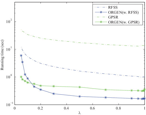
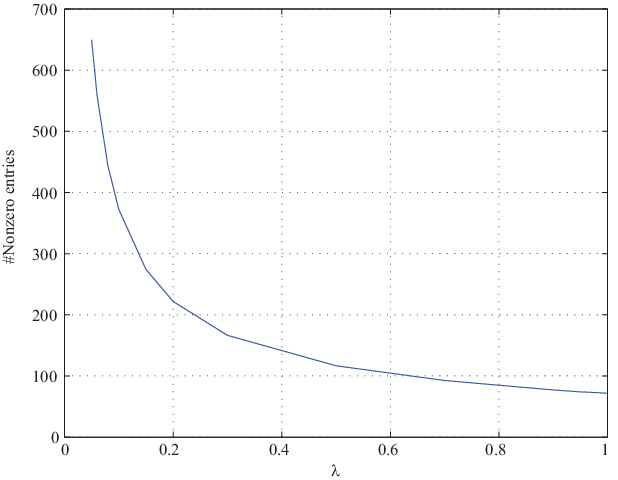
Next, we test the performance of ORGEN for various values of the parameter $\lambda$ that controls the tradeoff between the subspace preserving and connectedness properties; the running times and sparsity level are shown in Figures 5(b) and 5(c), respectively. The performance of SPAMS is not reported since it performs poorly even for moderately small values of $\lambda$. For all methods, the computational efficiency decreases as $\lambda$ becomes smaller. For the two versions of ORGEN, this is expected since the solution becomes denser as $\lambda$ becomes smaller (see Figure 5(c)). Thus the active sets become larger, which leads directly to larger and more time consuming subproblems in step 3.

In this section, we use ORGEN to solve the optimization problems arising in EnSC, where each subproblem in step 3 is solved using the RFSS method. To compute the coefficient vectors $\boldsymbol{c}^{*}(\boldsymbol{x}_{j},X_{-j})$, the parameter $\lambda$ is set to be the same for all $j$, while the parameter $\gamma$ is set as $\gamma=\alpha\gamma_{0}$ where $\alpha>1$ is a hyperparameter and $\gamma_{0}$ is the smallest value of $\gamma$ such that $\boldsymbol{c}^{*}(\boldsymbol{x}_{j},X_{-j})$ is nonzero. The algorithm is run for at most $2$ iterations, as we observe that this is sufficient for the purpose of subspace clustering and that subsequent iterations do not boost performance. We measure clustering performance by clustering accuracy, which is calculated as the best matching rate between the label predicted by the algorithm and that of the ground truth.

The second group consists of LRSC and SSC (with a different solver). We use the code provided by their respective authors, which uses the Alternating Direction Method of Multipliers (ADMM) to solve the optimization problems. To distinguish the two versions of SSC, we refer to this one as SSC-ADMM and to the previous one as SSC-SPAMS.

The final group consists of ENSC [32] and KMP [22], and are the closest in spirit to our method. Our method and ENSC both balance the $\ell_{1}$ and $\ell_{2}$ regularizations, but ENSC uses $h(\boldsymbol{e})=\|\boldsymbol{e}\|_{1}$ to penalize the noise (see (1)) and the linearized alternating direction method to minimize their objective. In KMP, the k-support norm is used to blend the $\ell_{1}$ and $\ell_{2}$ regularizers. We implemented ENSC and KMP according to the descriptions in their original papers.

We see that our proposed method achieves the best clustering performance on every dataset. Our method is also among the most efficient in terms of computing time. The methods SSC-ADMM, ENSC, LRSC and KMP cannot handle large-scale data because they perform calculations over the full data matrix and put the entire kernel matrix $X^{\top}X$ in memory, which is infeasible for large datasets. The method of SSC-SPAMS uses an active set method that can deal with massive data, however, it is computationally much less efficient than our solver ORGEN.

For understanding the advantages of our method, in Table 2 we report the sparsity of the representation coefficients, which is the number of nonzero entries in $\boldsymbol{c}_{j}$ averaged over all $j=1,\ldots,N$. For TSC, OMP and NSN, the sparsity is directly provided as a parameter of the algorithms. For SSC and our method EnSC-ORGEN, the sparsity is indirectly controlled by the parameters of the models. We can see that our method usually gives more nonzero entries than the sparsity based methods of TSC, OMP, NSN, and SSC. This shows the benefit of our method: while the number of correct connections built by OMP, NSN and SSC are in general upper-bounded by the dimension of the subspace, our method does not have this limit and is capable of constructing more correct connections and producing well-connected affinity graphs. On the other hand, the affinity graph of LRSC is dense, so although each cluster is self-connected, there are abundant wrong connections. This highlights the advantage of our method, which is flexible in controlling the number of nonzero entries by adjusting the trade-off parameter $\lambda$. Our results illustrate that this trade-off improves clustering accuracy.

Finally, ENSC and KMP are two representatives of other methods that also exploit the trade-off between $\ell_{1}$ and $\ell_{2}$ regularizations. A drawback of both works is that the solvers for their optimization problems are not as effective as our ORGEN algorithm, as they cannot deal with large datasets due to memory requirements. Moreover, we observe that their algorithms converge to modest accuracy in a few iterations but can be very slow in giving a high precision solution. This may explain why their clustering accuracy is not as good as that of EnSC-ORGEN. Especially, we see that ENSC gives dense solutions although the true solution is expected to be sparser, and this is explained by the fact that the solution paths of their solver are dense solutions.

References

- [1] A. Argyriou, R. Foygel, and N. Srebro. Sparse prediction with the -support norm. In Neural Information Processing Systems, pages 1466–1474, 2012.
- [2] A. Beck and M. Teboulle. A fast iterative shrinkage-thresholding algorithm for linear inverse problems. SIAM Journal on Imaging Sciences, 2(1):183–202, Mar 2009.
- [3] J. Bruna and S. Mallat. Invariant scattering convolution networks. IEEE Transactions on Pattern Analysis and Machine Intelligence, 35(8):1872–1886, 2013.
- [4] G. Chen and G. Lerman. Spectral curvature clustering (SCC). International Journal of Computer Vision, 81(3):317–330, 2009.
- [5] X. Chen and D. Cai. Large scale spectral clustering with landmark-based representation. In AAAI Conference on Artificial Intelligence, 2011.
- [6] J. Costeira and T. Kanade. A multibody factorization method for independently moving objects. International Journal of Computer Vision, 29(3):159–179, 1998.
- [7] C. De Mol, E. De Vito, and L. Rosasco. Elastic-net regularization in learning theory. Journal of Complexity, 25(2):201–230, 2009.
- [8] E. L. Dyer, A. C. Sankaranarayanan, and R. G. Baraniuk. Greedy feature selection for subspace clustering. Journal of Machine Learning Research, 14(1):2487–2517, 2013.
- [9] B. Efron, T. Hastie, I. Johnstone, and R. Tibshirani. Least angle regression. Annals of Statistics, 32(2):407–499, 2004.
- [10] E. Elhamifar and R. Vidal. Sparse subspace clustering. In IEEE Conference on Computer Vision and Pattern Recognition, 2009.
- [11] E. Elhamifar and R. Vidal. Sparse subspace clustering: Algorithm, theory, and applications. IEEE Transactions on Pattern Analysis and Machine Intelligence, 35(11):2765–2781, 2013.
- [12] Y. Fang, R. Wang, and B. Dai. Graph-oriented learning via automatic group sparsity for data analysis. In IEEE International Conference on Data Mining, pages 251–259, 2012.
- [13] Y. Fang, R. Wang, B. Dai, and X. Wu. Graph-based learning via auto-grouped sparse regularization and kernelized extension. IEEE Transactions on Knowledge and Data Engineering, 27(1):142–154, 2015.
- [14] P. Favaro, R. Vidal, and A. Ravichandran. A closed form solution to robust subspace estimation and clustering. In IEEE Conference on Computer Vision and Pattern Recognition, 2011.
- [15] M. Figueiredo, R. Nowak, and S. Wright. Gradient projection for sparse reconstruction: Application to compressed sensing and other inverse problems. IEEE Journal of Selected Topics in Signal Processing, 1(4):586–597, 2007.
- [16] E. Grave, G. Obozinski, and F. Bach. Trace lasso: a trace norm regularization for correlated designs. In Neural Information Processing Systems, 2011.
- [17] R. Gross, I. Matthews, J. F. Cohn, T. Kanade, and S. Baker. Multi-PIE. Image Vision Computing, 28(5):807–813, 2010.
- [18] R. Heckel and H. Bölcskei. Robust subspace clustering via thresholding. CoRR, abs/1307.4891, 2013.
- [19] J. Ho, M. H. Yang, J. Lim, K. Lee, and D. Kriegman. Clustering appearances of objects under varying illumination conditions. In IEEE Conference on Computer Vision and Pattern Recognition, 2003.
- [20] W. Hong, J. Wright, K. Huang, and Y. Ma. Multi-scale hybrid linear models for lossy image representation. IEEE Transactions on Image Processing, 15(12):3655–3671, 2006.
- [21] B. Jin, D. Lorenz, and S. Schiffler. Elastic-net regulariztion: error estimates and active set methods. Inverse Problems, 25(11), 2009.
- [22] H. Lai, Y. Pan, C. Lu, Y. Tang, and S. Yan. Efficient k-support matrix pursuit. In European Conference on Computer Vision, pages 617–631, 2014.
- [23] Y. LeCun, L. Bottou, Y. Bengio, and P. Haffner. Gradient-based learning applied to document recognition. Proceedings of the IEEE, 86(11):2278 – 2324, 1998.
- [24] C.-G. Li and R. Vidal. Structured sparse subspace clustering: A unified optimization framework. In IEEE Conference on Computer Vision and Pattern Recognition, pages 277–286, 2015.
- [25] Z. Lin, R. Liu, and Z. Su. Linearized alternating direction method with adaptive penalty for low rank representation. In Neural Information Processing Systems, 2011.
- [26] G. Liu, Z. Lin, S. Yan, J. Sun, and Y. Ma. Robust recovery of subspace structures by low-rank representation. IEEE Trans. Pattern Analysis and Machine Intelligence, 35(1):171–184, Jan 2013.
- [27] G. Liu, Z. Lin, and Y. Yu. Robust subspace segmentation by low-rank representation. In International Conference on Machine Learning, 2010.
- [28] C. Lu, Z. Lin, and S. Yan. Correlation adaptive subspace segmentation by trace lasso. In IEEE International Conference on Computer Vision, 2013.
- [29] C.-Y. Lu, H. Min, Z.-Q. Zhao, L. Zhu, D.-S. Huang, and S. Yan. Robust and efficient subspace segmentation via least squares regression. In European Conference on Computer Vision, 2012.
- [30] B. Nasihatkon and R. Hartley. Graph connectivity in sparse subspace clustering. In IEEE Conference on Computer Vision and Pattern Recognition, 2011.
- [31] S. A. Nene, S. K. Nayar, and H. Murase. Columbia object image library (COIL-100). Technical Report CUCS-006-96, 1996.
- [32] Y. Panagakis and C. Kotropoulos. Elastic net subspace clustering applied to pop/rock music structure analysis. Pattern Recognition Letters, 38:46–53, 2014.
- [33] D. Park, C. Caramanis, and S. Sanghavi. Greedy subspace clustering. In Neural Information Processing Systems, 2014.
- [34] X. Peng, L. Zhang, and Z. Yi. Scalable sparse subspace clustering. IEEE Conference on Computer Vision and Pattern Recognition, pages 430–437, 2013.
- [35] S. Rao, R. Tron, R. Vidal, and Y. Ma. Motion segmentation in the presence of outlying, incomplete, or corrupted trajectories. IEEE Transactions on Pattern Analysis and Machine Intelligence, 32(10):1832–1845, 2010.
- [36] M. Soltanolkotabi and E. J. Candès. A geometric analysis of subspace clustering with outliers. Annals of Statistics, 2013.
- [37] M. Tsakiris and R. Vidal. Filtrated spectral algebraic subspace clustering. In ICCV Workshop on Robust Subspace Learning and Computer Vision, pages 28–36, 2015.
- [38] R. Vidal. Subspace clustering. IEEE Signal Processing Magazine, 28(3):52–68, March 2011.
- [39] R. Vidal and P. Favaro. Low rank subspace clustering (LRSC). Pattern Recognition Letters, 43:47–61, 2014.
- [40] R. Vidal, Y. Ma, and S. Sastry. Generalized Principal Component Analysis (GPCA). IEEE Transactions on Pattern Analysis and Machine Intelligence, 27(12):1–15, 2005.
- [41] R. Vidal, Y. Ma, and S. Sastry. Generalized Principal Component Analysis. Springer Verlag, 2016.
- [42] R. Vidal, R. Tron, and R. Hartley. Multiframe motion segmentation with missing data using PowerFactorization, and GPCA. International Journal of Computer Vision, 79(1):85–105, 2008.
- [43] U. von Luxburg. A tutorial on spectral clustering. Statistics and Computing, 17, 2007.
- [44] Y.-X. Wang and H. Xu. Noisy sparse subspace clustering. In International Conference on Machine learning, 2013.
- [45] Y.-X. Wang, H. Xu, and C. Leng. Provable subspace clustering: When LRR meets SSC. In Neural Information Processing Systems, 2013.
- [46] C. You, D. Robinson, and R. Vidal. Scalable sparse subspace clustering by orthogonal matching pursuit. In IEEE Conference on Computer Vision and Pattern Recognition, 2016.
- [47] C. You and R. Vidal. Geometric conditions for subspace-sparse recovery. In International Conference on Machine Learning, pages 1585–1593, 2015.
- [48] C. You and R. Vidal. Subspace-sparse representation. Arxiv, abs/1507.01307, 2015.
- [49] T. Zhang, A. Szlam, Y. Wang, and G. Lerman. Hybrid linear modeling via local best-fit flats. International Journal of Computer Vision, 100(3):217–240, 2012.
- [50] H. Zou and T. Hastie. Regularization and variable selection via the elastic net. Journal of the Royal Statistical Society, Series B, 67:301–320, 2005.