Characterization and Inference of Graph Diffusion Processes from Observations of Stationary Signals

We consider a set of $N$ random variables (vertices) of interest. Our objective is, given a set of $M$ realizations (signals) of these variables, to infer a diffusion matrix adapted to the underlying graph topology on which unknown i.i.d. signals could have evolved to generate the given $M$ observations.

Graph shift operators are defined by Sandryhaila et al. [11, 12] as local operations that replace a signal value at each vertex of a graph with the linear combination of the signal values at the neighbors of that vertex. The adjacency matrix is an example of graph shift operator, as its entries are non-null if and only if there exists a corresponding edge in $\mathcal{E}$.

Graphs may have numerous properties that can be used as priors when inferring an unknown graph. In this paper, we are particularly interested in the sparsity of the graph, that measures the density of its edge, and in its simplicity. A graph is said to be simple if no vertex is connected to itself, i.e., if the diagonal entries of the associated adjacency matrix are null. These two properties are often desired in application domains. In the general case, we consider graphs that can have self-loops, i.e., non-null elements on the diagonal of W.

A signal on a graph can be seen as a vector that attaches a value to every vertex in $\mathcal{V}$.

A widely-considered matrix that allows the study of signals on a graph $\mathcal{G}$ is the normalized Laplacian of $\mathcal{G}$.

An interpretation of this matrix is obtained by considering the propagation of a signal x on $\mathcal{G}$ using Ł. By definition, $\textbf{\L}\textbf{x}=\textbf{I}\textbf{x}-(\textbf{D}^{-\frac{1}{2}}\textbf{W}\textbf{D}^{-\frac{1}{2}})\textbf{x}$. Therefore, the normalized Laplacian models the variation of a signal x when diffused through one step of a diffusion process represented by the graph shift operator $\textbf{T}_{\textbf{\L}}\triangleq\textbf{D}^{-\frac{1}{2}}\textbf{W}\textbf{D}^{-\frac{1}{2}}$. More generally, in this paper, we define diffusion matrices as follows:

The idea behind these constraints is that we want to model a diffusion process by a matrix. Such process propagates signal components from vertex to vertex and consequently consists of positive entries indicating what quantity of signal is sent to the neighboring vertices. Enforcing all eigenvalues to have their modulus be at most $1$ imposes a scale factor, and has the interesting consequence to cause the series $\left(\textbf{T}^{i}\textbf{x}\right)_{i}$ to be bounded, for any signal x.

Note that by construction, the largest eigenvalue of $\textbf{T}_{\textbf{\L}}$ is $1$. In our experiments, we will use this particular matrix $\textbf{T}_{\textbf{\L}}$ to diffuse signals on the graph. Other popular matrices could be used instead to diffuse signals. For example, any polynome of $\textbf{T}_{\textbf{\L}}$ could be used [13, 14, 15].

One of the cornerstones of signal processing on graphs is the analogy between the notion of frequency in classical signal processing and the eigenvalues of the Laplacian. The eigenvectors of the Laplacian of a binary ring graph correspond to the classical Fourier modes (see e.g., [16] for a detailed explanation). The lowest eigenvalues are analogous to low frequencies, while higher ones correspond to higher frequencies. Using this analogy, researchers have successfully been able to use graph signal processing techniques on non-ring graphs (e.g., [17, 18]).

To be able to do so, the Laplacian matrix of the studied graph must be diagonalizable. Although it is a sufficient, but not necessary, condition for diagonalization, we only consider undirected graphs in this article (see Definition 1), for which the normalized Laplacian as defined in Definition 3 is symmetric. Note that there also exist definitions of the Laplacian matrix when the graphs are directed [19].

To understand the link between diffusion of signals on the graph and the notion of smoothness on the graph introduced in Section II-C, we need to introduce the graph Fourier transform [20, 16], that transports a signal x defined on the graph into its spectral representation $\widehat{\textbf{x}}$:

This operator allows the transportation of signals into a spectral representation defined by the graph. Note that there exist other graph Fourier transform operators, based on the eigenvectors of the non-normalized Laplacian ${\bf L}\triangleq\textbf{D}-\textbf{W}$ or on those of the adjacency matrix [11].

An important property of the normalized Laplacian states that the eigenvalues of Ł lie in the closed interval [0, 2], with the multiplicity of eigenvalue $0$ being equal to the number of connected components in the graph, and $2$ being an eigenvalue for bipartite graphs only [20]. We obtain that the eigenvalues of $\textbf{T}_{\textbf{\L}}$ lie in the closed interval [-1, 1], with at least one of them being equal to $1$. Also, since $\textbf{T}_{\textbf{\L}}$ and Ł only differ by an identity, both matrices share the same set of eigenvectors. If the graph is connected then $\textbf{T}_{\textbf{\L}}$ has a single eigenvalue equal to $1$, being associated with a constant-sign eigenvector $\text{$\boldsymbol{\chi}$}_{1}$:

where D is the matrix of degrees introduced in Definition 3, and all other eigenvalues of $\textbf{T}_{\textbf{\L}}$ are strictly less than $1$.

Therefore, diffusing a signal x using $\textbf{T}_{\textbf{\L}}$ shrinks the spectral contribution of the eigenvectors of Ł associated with high eigenvalues more than those associated with lower ones.

It is worth noting that since one of the eigenvalues of $\textbf{T}_{\textbf{\L}}$ is equal to $1$, then the contribution of the associated eigenvector $\text{$\boldsymbol{\chi}$}_{1}$ does not change after diffusion. Therefore, after numerous diffusion steps, $\left(\text{$\text{$\widehat{\textbf{x}}$}(i)$}\right)_{i\in[2;\text{$N$}]}$ become close to null and x becomes stable on any non-bipartite graph. As a consequence, we consider in our experiments signals that are diffused a limited number of times.

A commonly desired property for signals on graphs is smoothness. Informally, a signal is said to be smooth on the graph if it has similar entries where the corresponding vertices are adjacent in the graph. In more details, given a diffusion matrix T for a graph $\mathcal{G}$, smoothness of a signal x can be measured via the following quantity:

From this equation, we can see that the lower $S(\textbf{x})$ is, the more regular are the entries of x on the graph. When using $\textbf{T}_{\textbf{\L}}$ as a diffusion matrix, signals that are low-frequency, i.e., that mostly have a spectral contribution of the lower eigenvectors of the Laplacian, have a low value of $S(\textbf{x})$ and are then smooth on the graph. As mentioned above, diffusion of signals using $\textbf{T}_{\textbf{\L}}$ shrinks the contribution of eigenvectors of Ł associated with higher eigenvalues more than the contribution of the ones associated with lower eigenvalues. Thence the property that diffused signals become low-frequency after some diffusion steps, and hence smooth on the graph. In addition to seeing diffusion as a link between graphs and signals naturally defined on them, this interesting property justifies the assumption, made in many papers, that signals should be smooth on a graph modeling their support [5, 6, 7].

Considering stationary signals is a very classical framework in traditional signal processing that facilitates the analysis of signals. Analogously, stationary processes on graphs have been recently defined to ease this analysis in the context of signal processing on graphs [8, 9, 10].

A random process on a graph is said to be (wide-sense) stationary if its first moment is constant over the vertex set and its covariance matrix is invariant with respect to the localization operator [10]. In particular, white noise is stationary for any graph, and any number of applications of a graph shift operator on such noise leaves the process stationary. This implies that the covariance matrix of stationary signals shares the same eigenvectors as this particular operator (see Section III-D for details).

Diffusion of signals is a particular case of stationary processing. The example we develop in this article when studying diffusion of signals through a matrix T can be generalized to any stationary process and any graph shift operator, with only few adaptations.

Using the previously introduced notions, we can formulate the problem we address in this paper as follows. Let $\textbf{X}=(\textbf{x}_{1},\dots,\textbf{x}_{\text{$M$}}),\textbf{x}_{i}\in\text{$\mathbb{R}$}^{\text{$N$}}$, be a $\text{$N$}\times\text{$M$}$ matrix of $M$ observations, one per column. Let $\textbf{Y}=(\textbf{y}_{1},\dots,\textbf{y}_{\text{$M$}}),\textbf{y}_{i}\in\text{$\mathbb{R}$}^{\text{$N$}}$, be a $\text{$N$}\times\text{$M$}$ unknown matrix of $M$ i.i.d. signals; i.e., the entries $\textbf{Y}(i,j)$ are zero-mean, independent random variables. Let $\textbf{k}\in\text{$\mathbb{R}$}_{+}^{\text{$M$}}$ be an unknown vector of $M$ positive numbers, corresponding to the number of times each signal is diffused before observation.

Given X, we aim to characterize the set of all diffusion matrices¹¹ 1 Throughout this article we will denote recovered/estimated quantities using a tilde. $\widetilde{\textbf{T}}$ such that there exist Y and k with:

This framework can be seen as a particular case of graph filters [12], containing only a monomial of the diffusion matrix. From a practical point of view, this corresponds to the setup where all signals are observed at a given time $t$, but have been initialized at various instants $t-\text{$\textbf{k}(i)$}$. More generally, all polynomials of the diffusion matrix share the same eigenvectors. The key underlying assumption in our work is that each observation is the result of passing white noise through a graph filter whose eigenvectors are the same as those of the normalized Laplacian. Consequently, our approach can be applied to any graph filter

for $M$ sequences $\mathcal{K}_{1},\dots,\mathcal{K}_{\text{$M$}}$.

To summarize the following sections, we infer a diffusion matrix in two steps. First, we characterize the convex set of solutions using the method in Section IV. Then, we select a point from this set using some criteria on the matrix we want to infer. The strategies we propose are given in Section V.

As stated in the introduction, obtaining the eigenvectors of the covariance matrix is a cornerstone of our approach. They allow us to define a polytope limiting the set of matrices that can be used to model a diffusion process.

Since the covariance matrix $\text{$\boldsymbol{\Sigma}$}\triangleq\text{$\mathbb{E}\left[\textbf{X}\text{$\textbf{X}^{\top}$}\right]$}$ is not obtainable in practical cases, a common approach involve estimating $\boldsymbol{\Sigma}$ using the sample covariance matrix $\widetilde{\text{$\boldsymbol{\Sigma}$}}$:

where $\textbf{M}(i,j)\triangleq\frac{1}{\text{$M$}}\sum\limits_{k=1}^{\text{$M$}}\textbf{X}(i,k)$ is an $\text{$N$}\times\text{$M$}$ matrix with each row containing the mean signal value for the associated vertex. An interesting property of this matrix is that its eigenvectors converge to those of the covariance matrix as the number of signals increases (see Section IV-B).

Other methods exist to infer a covariance matrix [23, 24, 25, 26] and may be interesting to consider in place of the sample covariance matrix. Methods for retrieving a sparse covariance matrix based on properties of its spectral norm are described in [23] and [24]. However, these works do not provide any information on the convergence rate of the eigenvectors of their solutions to the eigenvectors of the covariance matrix, as the number of signals increases. Similarly, [25] and [26] retrieve covariance matrices that converge in operator norm or in distribution. An intensive study of covariance estimation methods could be interesting to find techniques that improve the convergence of eigenvectors. This paper focuses on the use of the sample covariance matrix.

A widely-used approach to provide a graph is the graphical lasso [27], which recovers a sparse precision matrix (i.e., inverse covariance matrix) $\widetilde{\text{$\boldsymbol{\Theta}$}}$ under the assumption that the data are observations from a multivariate Gaussian distribution. The core of this method consists in solving the following problem,

where $\widetilde{\text{$\boldsymbol{\Sigma}$}}$ is the sample covariance matrix and $\lambda$ is a regularization parameter controlling sparsity.

Numerous variations of this technique have been developed [28, 29, 30, 31], and several applications have been using graphical lasso-based methods for inferring a sparse graph. Examples can be found for instance in the fields of neuroimaging [32, 33] or traffic modeling [34].

What makes this method interesting, in addition to its fast convergence to a sparse solution, is a previous result from Dempster [3]. In the covariance selection model, Dempster proposes that the inverse covariance matrix should have numerous null off-diagonal entries. An additional result from Wermuth [35] states that the non-null entries in the precision matrix correspond to existing edges in a graph that is representative of the studied data.

Therefore, in our experiments, we evaluate whether considering the result of the graphical lasso as a graph makes it admissible or not to model a diffusion process. However, when considering (6), we can see that the method does not impose any similarity between the eigenvectors of the covariance matrix and those of the inferred solution. For this reason, we do not expect this method to provide a solution that is admissible in our settings.

Close to the graphical lasso, [36] and [37] propose an algorithm to infer a precision matrix by adding generalized Laplacian constraints. While this allows for good recovery of the precision matrix, it proceeds in an iterative way by following a block descent algorithm that updates one row/column per iteration. As for the graphical lasso, it does not force the eigenvectors of the retrieved matrix to match those of the covariance matrix, and therefore does not match our stationarity assumption. Interestingly, these methods could also be mentioned in the next section, dedicated to smoothness-based methods. In particular, [36] has pointed out that minimizing the quantity $\trace(\text{$\text{$\widetilde{\text{$\boldsymbol{\Sigma}$}}$}$}\text{$\boldsymbol{\Theta}$})$ promotes smoothness of the solution when $\boldsymbol{\Theta}$ is a graph Laplacian. Additionally, [38] promotes sparsity of the inferred graph by applying a soft threshold to the precision matrix, and shows that the solution matches a smoothness assumption on signals.

Another approach to recover a graph is to assume that the signal components should be similar when the vertices on which they are defined are linked with a strong weight in W, thus enforcing natural signals on this graph to be low-frequency (smooth). Using the definition of smoothness of signals on a graph in (2), we can see that the smaller $S(\textbf{x})$, the more regular the components of x on the graph.

A first work taking this approach has been proposed by Lake and Tenenbaum [5], in which they solve a convex optimization problem to recover a sparse graph from data to learn the structure best representing some concepts. More recently, Dong et al. [6] have proposed a similar method that outperforms the one by Lake and Tenenbaum. In order to find a graph Laplacian that minimizes $S$ in (2) for a set of signals, the authors propose an iterative algorithm that converges to a local solution, based on the resolution of the following problem:

where $\textbf{L}^{*}$ is the non-normalized Laplacian recovered, $\|\cdot\|_{F}$ is the Frobenius norm, Y is a matrix in $\text{$\mathbb{R}$}^{\text{$N$}\times\text{$M$}}$ that can be considered as a noiseless version of signals X, and $\alpha$ and $\beta$ are regularization parameters controlling the distance between X and Y, and the sparsity of the solution.

Kalofolias [7] proposes a unifying framework to improve the previous solutions of Lake and Tenenbaum, and Dong et al., by proposing a better prior and reformulating the problem to optimize over entries of the (weighted) adjacency matrix rather than the Laplacian. An efficient implementation of his work is provided in the Graph Signal Processing Toolbox [39]. His approach consists in rewriting the problem as an $\ell_{1}$ minimization, that leads to naturally sparse solutions. Moreover, the author has shown that the method from Dong et al. could be encoded in his framework.

Graph inference with smoothness priors continues to receive a lot of interest. Recently, Chepuri et al. [40] have proposed to infer a sparse graph on which signals are smooth, using an edge selection strategy. Finally, enforcing the smoothness property for signals defined on a graph has also been considered by Shivaswamy and Jebara [41], where a method is proposed to jointly learn the kernel of an SVM classifier and optimize the spectrum of the Laplacian to improve this classification. Contrary to our approach, Shivaswamy and Jebara [41] study a semi-supervised case, in which the spectrum of the Laplacian is learned based on a set of labeled examples.

Recently we proposed a third approach to recover a graph from diffused signals. In [42], we study a particular case of the problem we consider here, namely when k is a known constant vector. Let $K$ denote the value in every entry of this vector. We show in [42] that the covariance matrix of signals diffused $K$ times on the graph is equal to $\textbf{T}^{2\text{$K$}}$. This implies that we need to recover a particular root of the covariance matrix to obtain T. In more details, if Y is a matrix of mutually independent signals with independent entries, $\textbf{X}=\textbf{T}^{\text{$K$}}\textbf{Y}$, and $\boldsymbol{\Sigma}$ is the covariance matrix of X, we have:

using the independence of Y and the symmetry of T.

Thanks to $K$ being known, one could then retrieve a matrix $\widetilde{\textbf{T}}$ by diagonalizing $\boldsymbol{\Sigma}$, taking the $2\text{$K$}$-square root of the obtained eigenvalues, and solving a linear optimization problem to recover their missing signs. This reconstruction process was illustrated on synthetic cases, where a graph $\mathcal{G}$ is generated, and $M$ i.i.d. signals are diffused on it using the associated matrix $\textbf{T}^{\text{$K$}}$ to obtain X[42]. Experiments demonstrate that when using $\text{$\text{$\widetilde{\text{$\boldsymbol{\Sigma}$}}$}$}=\textbf{T}^{2\text{$K$}}$ (which is the limit case when $M$ grows to infinity), we can successfully recover $\text{$\text{$\widetilde{\textbf{T}}$}$}=\textbf{T}$.

However, this previous work has two principal limitations:

1. 1.

   The number of diffusion steps k is constant and known, which is a limiting assumption since in practical applications signals may be obtained after a variable, unknown number of diffusion steps. In this work, we remove this assumption. Taking the $2\text{$K$}$-square root of the eigenvalues of $\boldsymbol{\Sigma}$ is therefore no longer possible.

2. 2.

   The number of observations $M$ is assumed to be infinite so that we have a perfect characterization of the eigenvectors of the covariance matrix. We also address this assumption in this paper and show that the higher $M$, the closer the recovered graph to the ground truth.

Ongoing work by Segarra et al. [43, 44], initiated in [45], takes a similar direction. The authors propose a two-step approach, where they first retrieve the eigenvectors of a graph shift operator, and then infer the missing eigenvalues based on some criteria. They also study the case of stationary graph processes, for which the covariance matrix shares the same eigenbasis as the graph Fourier transform operator, and use this information to infer a graph based on additional criteria.

However, while the characterization of the set of solutions is identical to ours, our works differ in the matrix selection strategy. Segarra et al. [43] focus on adjacency and Laplacian inference, while we aim at recovering a matrix modeling a diffusion process. Still, note that both of our works can be easily extended to any graph shift operator, by setting up the correct set of constraints. The authors of [43] solve a slightly different problem, where they minimize the $\ell_{1}$ norm of the inferred matrix under more constraints than ours, which describe a valid Laplacian matrix. In particular, they enforce the diagonal elements of the solution to be null, thus considering graphs that do not admit self-loops. In more details, they solve the following optimization problem:

where ${\bf S}^{*}$ is the inferred graph shift operator, $\mathcal{S}$ is the set of admissible solutions delimited by their constraints, and $\text{$\boldsymbol{\chi}$}_{1},\dots,\text{$\boldsymbol{\chi}$}_{\text{$N$}}$ are the eigenvectors of the covariance matrix. Contrary to their approach, we aim at inferring a matrix that can be simple (see Section V-A) or sparse (see Section V-B), rather than selecting a sparse matrix from the set of simple matrices. Among other differences, we propose in Section V-C a method to approximate the solution of any graph inference strategy to make it match our stationary assumption on signals. Our work also explores how the polytope of solutions can be used to evaluate which graph, among a set of given graphs, is the most adapted to given signals.

Shahrampour and Preciado [46, 47] study the context of network inference from stimulation of its vertices with noise. However, their method implies a series of node knockout operations that need to individually intervene on the vertices.

Also, we note that there exist methods that aim to recover a graph from the knowledge of its Laplacian spectrum [48]. However, we do not assume that such information is available.

Finally, a recent work by Shafipour et al. [49] has started to explore the problem of graph inference from non-stationary graph signals, which is a direct continuation of the work presented in this article and of the work by Segarra et al..

In the asymptotic case when $M$ is infinite, the covariance matrix $\boldsymbol{\Sigma}$ of the given signals X is equal to a (fixed) power $K$ of the diffusion matrix. Thus, under these asymptotic settings, $\boldsymbol{\mathcal{X}}$ can be obtained using Principal Component Analysis on X [50]. In the more global case when k is a vector, the covariance matrix of the signals is a linear combination of multiple powers of T, and has therefore the same set of eigenvectors, since all powers of a matrix share the same eigenvectors. This is also the case when considering graph filters as in (4).

In more details, if we consider signals $\textbf{x}_{i}=\textbf{T}^{\text{$\textbf{k}(i)$}}\textbf{y}_{i}$, we have the following development. We denote by $\textbf{X}(i)$ the signal at the $i^{\text{th}}$ column of X, and drop the constant factor and signals mean from (5) for readability:

which is a linear combination of various powers of T, all having the same eigenvectors $\boldsymbol{\mathcal{X}}$.

Let us first consider the limit case when the eigenvectors $\boldsymbol{\mathcal{X}}$ of $\boldsymbol{\Sigma}$ are available. Given the remarks in Section II-B, to recover an acceptable diffusion matrix $\widetilde{\textbf{T}}$, we must find eigenvalues $\text{$\text{$\widetilde{\text{$\boldsymbol{\Lambda}$}}$}$}=(\text{$\text{$\widetilde{\text{$\lambda$}_{1}}$}$},\dots,\text{$\text{$\widetilde{\text{$\lambda$}_{\text{$N$}}}$}$})$ such that:

• •

  $\forall i,j\in\{1,\ldots,\text{$N$}\};j\geq i:\text{$\text{$\text{$\widetilde{\textbf{T}}$}$}(i,j)$}\geq 0$;

• •

  Let $\text{$\boldsymbol{\chi}$}_{1}$ be the constant-sign eigenvector in $\boldsymbol{\mathcal{X}}$: $\text{$\text{$\widetilde{\text{$\lambda$}_{1}}$}$}=1$;

• •

  $\forall i\in\{1,\ldots,\text{$N$}\}:\text{$\text{$\widetilde{\text{$\lambda$}_{i}}$}$}\in[-1,1]$.

Note that these constraints are driven by the will to recover a diffusion matrix as defined in Definition 4. If we were considering the case of other graph shift operators, these constraints would be different and would yield the definition of different constraints in (13). As an example, diffusion using a Laplacian matrix would imply the definition of constraints that enforce the diagonal entries to be positive and off-diagonal ones to be negative (see [43]). Similarly, aiming to recover the diffusion matrix $\textbf{T}_{\textbf{\L}}\triangleq\textbf{D}^{-\frac{1}{2}}\textbf{W}\textbf{D}^{-\frac{1}{2}}$ associated with the normalized Laplacian would imply additional constraints.

To illustrate how these properties translate into a set of admissible diffusion matrices, let us consider the randomly generated $3\times 3$ symmetric adjacency matrix $\textbf{W}=\begin{pmatrix}0.417\penalty\ &0.302\penalty\ &0.186\\ 0.302\penalty\ &0.147\penalty\ &0.346\\ 0.186\penalty\ &0.346\penalty\ &0.397\\ \end{pmatrix}$. We compute its associated matrix $\textbf{T}_{\textbf{\L}}$ and corresponding eigenvectors $\boldsymbol{\mathcal{X}}$. This simulates a perfect retrieval of the eigenvectors of the covariance matrix of signals diffused by $\textbf{T}_{\textbf{\L}}$ on the graph. For all pairs $(\text{$\text{$\widetilde{\text{$\lambda$}_{2}}$}$},\text{$\text{$\widetilde{\text{$\lambda$}_{3}}$}$})\in[-1,1]\times[-1,1]$ (using a step of $10^{-2}$), Fig. 1 depicts those that allow the reconstruction of a diffusion matrix.

As we can see, the set of admissible matrices is convex (but non-strictly convex), delimited by affine equations. To characterize these equations, let us consider any entry of index $(i,j)$ in the upper triangular part of the matrix $\widetilde{\textbf{T}}$ we want to recover. Since $\boldsymbol{\mathcal{X}}$ is assumed to be known, by developing the matrix product $\text{$\text{$\widetilde{\textbf{T}}$}$}\triangleq\text{$\boldsymbol{\mathcal{X}}$}\begin{pmatrix}\text{$\text{$\widetilde{\text{$\lambda$}_{1}}$}$}&0&0\\ 0&\dots&0\\ 0&0&\text{$\text{$\widetilde{\text{$\lambda$}_{\text{$N$}}}$}$}\end{pmatrix}\text{$\text{$\boldsymbol{\mathcal{X}}$}^{\top}$}$, we can write every entry $\text{$\text{$\widetilde{\textbf{T}}$}$}(i,j)$ as a linear combination of variables $\text{$\text{$\widetilde{\text{$\lambda$}_{1}}$}$},\dots,\text{$\text{$\widetilde{\text{$\lambda$}_{N}}$}$}$ by developing the scalars in $\boldsymbol{\mathcal{X}}$. Let $\alpha_{ij1},\dots,\alpha_{ij\text{$N$}}$ be the factors associated with $\text{$\lambda$}_{1},\dots,\text{$\lambda$}_{N}$ for the equation associated with the entry $\text{$\text{$\widetilde{\textbf{T}}$}$}(i,j)$, i.e.:

As an example, let us consider a $3\times 3$ matrix T with known eigenvectors $\boldsymbol{\mathcal{X}}$. Using the decomposition of T, we can write $\textbf{T}(2,3)$ as follows:

Enforcing the value of all entries of the matrix to be positive thus defines the following set of $\frac{\text{$N$}(\text{$N$}+1)}{2}$ inequalities:

where $j\geq i$ comes from the symmetry property.

Our problem of recovering the correct set of eigenvalues to reconstruct the diffusion matrix thus becomes a problem of selecting a vector of dimension $\text{$N$}-1$ (since one eigenvalue is equal to $1$ due to the imposed scale) in the convex polytope delimited by (13). Since the number of possible solutions is infinite, it is an ill-posed problem. To cope with this issue, one then needs to incorporate additional information or a selection criterion to enforce desired properties on the reconstructed matrix. To illustrate the selection of a point in the polytope, Section V presents strategies based on different criteria, namely sparsity and simplicity.

Note that the polytope is in most cases not a singleton. The covariance matrix belongs to the set of admissible matrices, along with all its powers, which are different if the covariance matrix is not the identity. When additional constraints delimit the polytope, for example when enforcing the matrices to be simple, there exist situations when the solution is unique [43].

The results discussed above use the eigenvectors $\boldsymbol{\mathcal{X}}$ of the limit covariance matrix $\boldsymbol{\Sigma}$ as $M$ tends to infinity, directly obtained by diagonalizing the diffusion matrix of a ground truth graph under study. Next, we study the impact of the use of the sample covariance matrix $\widetilde{\text{$\boldsymbol{\Sigma}$}}$ of controlled signals respecting our assumptions on the estimation of these eigenvectors.

To understand the impact of using $\widetilde{\text{$\boldsymbol{\Sigma}$}}$ instead of $\boldsymbol{\Sigma}$, let us again consider an example $3\times 3$ matrix and the associated polytope, as we did in Section IV-A. We generate a random graph with $\text{$N$}=3$ vertices by drawing the entries of its adjacency matrix uniformly, and compute its matrix $\textbf{T}_{\textbf{\L}}$. Using $\textbf{T}_{\textbf{\L}}$, we diffuse $M$ i.i.d. signals (entries are drawn uniformly) a variable number of times (chosen uniformly in the interval [2, 5]) to obtain X. Then, we compute the sample covariance matrix of X, $\widetilde{\text{$\boldsymbol{\Sigma}$}}$, and its matrix of eigenvectors $\widetilde{\text{$\boldsymbol{\mathcal{X}}$}}$.

Fig. 2 depicts in white the ground truth polytope (i.e., the one delimited by equations (13) using the eigenvectors of $\boldsymbol{\Sigma}$) and the polytopes associated with $10$ different sample covariance matrices $\widetilde{\text{$\boldsymbol{\Sigma}$}}$, obtained from different realizations of X. From each of the eigenvector sets of these empirical covariance matrices, we determine the pairs $(\text{$\text{$\widetilde{\text{$\lambda$}_{2}}$}$},\text{$\text{$\widetilde{\text{$\lambda$}_{3}}$}$})$ that satisfy the criteria in Section IV-A. Then, we plot a histogram of the number of occurrences of these valid pairs.

As we can see, the recovered polytope more accurately reflects the true one as $M$ increases. This coincides with the fact that the empirical covariance matrix converges to the real one as $M$ tends to infinity.

In more details, we are interested in the convergence of the eigenvectors of the empirical covariance matrix $\text{$\text{$\widetilde{\text{$\boldsymbol{\mathcal{X}}$}}$}$}=\{\text{$\text{$\widetilde{\text{$\boldsymbol{\chi}$}_{1}}$}$},\dots,{\text{$\text{$\widetilde{\text{$\boldsymbol{\chi}$}}$}$}_{\text{$N$}}}\}$ to those of the actual covariance matrix $\boldsymbol{\mathcal{X}}$. Asymptotic results on this convergence are provided by Anderson [51], which extends earlier related results by Girshick [52] and Lawley [53]. Let $\textbf{e}_{i}\triangleq\text{$\text{$\boldsymbol{\mathcal{X}}$}^{\top}$}\text{$\text{$\widetilde{\text{$\boldsymbol{\chi}$}_{i}}$}$}$ be the vector of cosine similarities between $\widetilde{\text{$\boldsymbol{\chi}$}_{i}}$ and all eigenvectors of the actual covariance matrix. Anderson [51] states that, as the number of observations tends to infinity, entries in $\textbf{e}_{i}$ have a Gaussian distribution with a known variance. In particular, when all eigenvalues are distinct, the inner product between the $i^{\text{th}}$ (for all $i$) eigenvector of the covariance matrix, $\text{$\boldsymbol{\chi}$}_{i}$, and the $j^{\text{th}}$ (for all $j$) eigenvector of its estimate, $\widetilde{\text{$\boldsymbol{\chi}$}_{j}}$, is asymptotically Gaussian with zero mean and variance

where $\text{$\lambda$}_{i}$ is the eigenvalue associated with $\text{$\boldsymbol{\chi}$}_{i}$, and $\widetilde{\text{$\lambda$}_{j}}$ is the eigenvalue associated with $\widetilde{\text{$\boldsymbol{\chi}$}_{j}}$. As a consequence, the variance decreases like $\frac{1}{\text{$M$}}$, and it also depends on the squared difference between $\text{$\lambda$}_{i}$ and $\widetilde{\text{$\lambda$}_{j}}$. Additionally, [51] shows that the maximum likelihood estimate $\widetilde{\text{$\lambda$}_{i}}$ of $\text{$\lambda$}_{i}$ (for all $i$) is

where $\text{$Q$}_{i}$ is the multiplicity of eigenvalue $\text{$\lambda$}_{i}$, and $\mathcal{L}_{i}$ is the set of integers {$\text{$Q$}_{1}+\dots+\text{$Q$}_{i-1}+1,\dots,\text{$Q$}_{1}+\dots+\text{$Q$}_{i}$}, containing all indices of equal eigenvalues. In the simple case when all eigenvalues are distinct, (15) simplifies to

The eigenvalues of the empirical covariance matrix thus converge to those of the actual covariance matrix as $M$ increases. As $M$ tends to infinity, $\textbf{e}_{i}$ thus tends to the $i^{\text{th}}$ canonical vector, indicating collinearity between $\widetilde{\text{$\boldsymbol{\chi}$}_{i}}$ and $\text{$\boldsymbol{\chi}$}_{i}$. Additionally, [51] provides a similar result for the more general case when eigenvalues may be repeated.

As we can see from (14), the convergence of the eigenvectors of the sample covariance matrix to the eigenvectors of the true covariance matrix is impacted by the eigenvalues of the matrix used to diffuse the signals. We know that diffusing a signal $K$ times using T is equivalent to $\textbf{T}^{\text{$K$}}\textbf{x}$. When rewriting this equation in the spectral basis, we obtain $(\text{$\boldsymbol{\mathcal{X}}$}\text{$\boldsymbol{\Lambda}$}^{K}\text{$\text{$\boldsymbol{\mathcal{X}}$}^{\top}$})\textbf{x}$, where $\boldsymbol{\mathcal{X}}$ and $\boldsymbol{\Lambda}$ are the eigenvectors and eigenvalues of T. As we can see, the power distributes on the eigenvalues, and due to their location in the interval $]-1,1]$ (with the noticeable exception of bipartite graphs), the term $(\text{$\lambda$}_{i}-\text{$\text{$\widetilde{\text{$\lambda$}_{j}}$}$})^{2}$ in (14) gets smaller, and $M$ must grow to achieve the same precision.

To illustrate the impact of the number of diffusions on the convergence of the polytope, let us consider the following experiment. We generate $10^{4}$ occurrences of random adjacency matrices of $\text{$N$}=10$ vertices, by drawing their entries uniformly in [0, 1], and enforcing symmetry. Then, for each adjacency matrix, we compute the associated matrix $\textbf{T}_{\textbf{\L}}$, and for various values of $K$ and of $M$, we diffuse $M$ randomly generated signals $K$ times using $\textbf{T}_{\textbf{\L}}$. From the diffused signals, we compute the eigenvectors of the sample covariance matrix, and check if the eigenvalues of $\textbf{T}_{\textbf{\L}}$ are located in the polytope defined by these eigenvectors. Fig. 3 depicts the ratio of times it is the case, for each combination of $K$ and $M$.

The figure demonstrates that the number of diffusions has some imporance in the process. Too small values of $K$ encode too little information on the diffusion matrix in the signals, but values that are too high concentrate the eigenvalues too much around $0$. This corroborates that, as the eigenvalues concentrate around $0$, it is necessary to have a higher value of $M$ to achieve the same precision.

The first criterion we consider to select a point in the polytope is simplicity of the solution. In other words, we want to encourage the retrieval of a set $\widetilde{\text{$\boldsymbol{\Lambda}$}}$ of eigenvalues that, jointly with the eigenvectors $\boldsymbol{\mathcal{X}}$ of the covariance matrix, produce a diffusion matrix that has an empty diagonal. Such a matrix represents a process that maximizes the diffusion of a signal evolving on it, and does not retain any of its energy.

As shown in Section IV-A, since we are considering a diffusion matrix as defined in Definition 4, the polytope of solutions is defined by inequality constraints (13) that each enforce the positivity of an entry in the matrix to recover. A consequence is that if the matrix to be retrieved contains any null entry, then the point we want to select lies on an edge or a face of the polytope, since at least one inequality constraint holds with equality. Enforcing simplicity of the solution is therefore equivalent to selecting a point in the polytope that is located at the intersection of at least $N$ constraints. Using this observation and the fact that the trace of a matrix is equal to the sum of its eigenvalues, retrieving the eigenvalues that enforce simplicity of the corresponding matrix reduces to solving a linear programming problem, stated as follows:

where the two last constraints impose a scale factor.

Equation (17) is a linear program for which it is known that polynomial-time algorithms exist. The main bottleneck of this method is the definition of the $\frac{\text{$N$}(\text{$N$}+1)}{2}$ linear constraints in (13), that are computed in $\mathcal{O}(\text{$N$}^{3})$ time and space.

In many applications one may believe the graph underlying the observations is sparse. Similar to the case when trying to recover a simple graph, finding a sparse admissible solution can be formulated as finding a point at the intersection of multiple linear constraints. To find a sparse solution, we seek the set of admissible eigenvalues for which the maximum number of constraints in (13) are null. This reduces to minimizing the $\ell_{0}$ norm of the solution, which is an NP-hard problem [54].

A common approach to circumvent this problem is to approximate the minimizer of the $\ell_{0}$ norm by minimizing the $\ell_{1}$ norm instead [55, 56, 57]. In our case, we use the $L_{1,1}$ matrix norm, which is the sum of all entries, since they are all positive. In this section, we adopt this approach and consider again a linear programming problem as follows:

where $\textbf{1}_{\text{$N$}}$ is the vector of $N$ entries all equal to one.

The two methods introduced before consist in selecting a point in the polytope, given simplicity or sparsity priors. In this section, we take a different point of view. Many graph inference techniques exist in the literature (see Section III), all enforcing different properties of the graph that is retrieved. However, most of them do not impose the eigenvectors of the inferred solution to match those of the covariance matrix. The idea here is to adapt these solutions to stationary signals.

To do so, let us consider an inference method $m$ providing an adjacency or a Laplacian matrix from a set of signals $\textbf{X}=(\textbf{x}_{1},\dots,\textbf{x}_{\text{$M$}})$. Let $\textbf{T}_{m}$ be a diffusion matrix associated with the inferred matrix (for example, the one derived from the normalized Laplacian). Let $\text{$\boldsymbol{\mathcal{X}}$}_{\textbf{T}_{m}}$ be the eigenvectors of $\textbf{T}_{m}$, and let $\text{$\boldsymbol{\mathcal{X}}$}_{\text{$\boldsymbol{\Sigma}$}}$ be the eigenvectors of the covariance matrix.

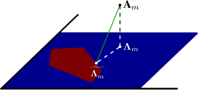
The idea here is to consider $\textbf{T}_{m}$ as if it were expressed in the eigenbasis of $\text{$\boldsymbol{\mathcal{X}}$}_{\text{$\boldsymbol{\Sigma}$}}$, to check whether it belongs or not to the polytope of admissible matrices. In other words, we want to find a matrix $\textbf{A}_{m}$ such that $\textbf{T}_{m}=\text{$\boldsymbol{\mathcal{X}}$}_{\text{$\boldsymbol{\Sigma}$}}\textbf{A}_{m}\text{$\boldsymbol{\mathcal{X}}$}_{\text{$\boldsymbol{\Sigma}$}}^{\top}$. Using the fact that $\text{$\boldsymbol{\mathcal{X}}$}_{\text{$\boldsymbol{\Sigma}$}}$ forms an orthonormal basis, we have $\textbf{A}_{m}=\text{$\boldsymbol{\mathcal{X}}$}_{\text{$\boldsymbol{\Sigma}$}}^{\top}\textbf{T}_{m}\text{$\boldsymbol{\mathcal{X}}$}_{\text{$\boldsymbol{\Sigma}$}}$. Unless $\text{$\boldsymbol{\mathcal{X}}$}_{\textbf{T}_{m}}$ and $\text{$\boldsymbol{\mathcal{X}}$}_{\text{$\boldsymbol{\Sigma}$}}$ are the same, $\textbf{A}_{m}$ is not necessarily a diagonal matrix. Therefore, $\textbf{A}_{m}$ lies in a space of dimension $\text{$N$}^{2}$, while the polytope is defined by $N$ variables.

Let us call $\text{$\boldsymbol{\Lambda}$}_{m}=(\text{$\lambda$}_{m_{1}},\dots,\text{$\lambda$}_{m_{\text{$N$}}})$ the vector of elements on the diagonal of $\textbf{A}_{m}$. Since the polytope of admissible diffusion matrices is defined in $\text{$\mathbb{R}$}^{\text{$N$}}$, $\text{$\boldsymbol{\Lambda}$}_{m}$ is the point of this set that forms the best estimate for $\textbf{A}_{m}$, defined in $\text{$\mathbb{R}$}^{\text{$N$}^{2}}$, after dimensionality reduction. In other words, $\text{$\boldsymbol{\Lambda}$}_{m}$ is the orthogonal projection of $\textbf{A}_{m}$ in the polytope. If $\text{$\boldsymbol{\Lambda}$}_{m}$ does not belong to the polytope of admissible diffusion matrices characterized by $\text{$\boldsymbol{\mathcal{X}}$}_{\text{$\boldsymbol{\Sigma}$}}$, then the method $m$ provides a solution that does not satisfy the conditions to be a diffusion process. To find the point in the polytope that is the closest to $\text{$\boldsymbol{\Lambda}$}_{m}$ in the sense of the Euclidean norm, we solve the following problem:

The solution to (19) gives us a set of eigenvalues $\text{$\text{$\widetilde{\text{$\boldsymbol{\Lambda}$}_{m}}$}$}=(\text{$\text{$\widetilde{\text{$\lambda$}_{m_{1}}}$}$},\dots,\text{$\text{$\widetilde{\text{$\lambda$}_{m_{\text{$N$}}}}$}$})$ that represent the best approximation of $\textbf{A}_{m}$ when restricting the search to admissible diffusion matrices. Therefore, the matrix $\text{$\text{$\widetilde{\textbf{T}_{m}}$}$}=\text{$\boldsymbol{\mathcal{X}}$}_{\text{$\boldsymbol{\Sigma}$}}\begin{pmatrix}\text{$\text{$\widetilde{\text{$\lambda$}_{m_{1}}}$}$}&0&0\\ 0&\dots&0\\ 0&0&\text{$\text{$\widetilde{\text{$\lambda$}_{m_{\text{$N$}}}}$}$}\end{pmatrix}\text{$\boldsymbol{\mathcal{X}}$}_{\text{$\boldsymbol{\Sigma}$}}^{\top}$ is the adaptation of the solution of method $m$ to stationary signals. We measure the distance between $\textbf{A}_{m}$, the projection of $\textbf{T}_{m}$ in the space defined by $\text{$\boldsymbol{\mathcal{X}}$}_{\text{$\boldsymbol{\Sigma}$}}$, and $\widetilde{\text{$\boldsymbol{\Lambda}$}_{m}}$, the closest point in the polytope, as follows:

where $\|\cdot\|_{F}$ is the Frobenius norm.

Fig. 4 summarizes provides a graphical illustration of the various steps to compute this distance.

In our experiments, we consider randomly generated graphs, produced by a random geometric model. These are frequently used to model connectivity in wireless networks [58].

Note that, by construction, such graphs are simple and relatively sparse. Therefore, we expect methods using such selection criteria to be able to retrieve them.

In some of our experiments, we also consider random graphs generated by an Erdős-Rényi model [59], in which two vertices are linked with a given probability independently from each other. Such graphs are defined as follows:

Once a graph is generated using the model presented above, and given a number $M$ of signals to produce, signals verifying our settings are created as follows:

1. 1.

   Create Y a $\text{$N$}\times\text{$M$}$ matrix with i.i.d. entries. We denote by $\textbf{Y}(i)$ the $i^{\text{th}}$ column of Y. In these experiments, entries of Y are drawn uniformly.

2. 2.

   Create k a vector of $M$ i.i.d. integer entries, comprised in the interval $\{1,\ldots,10\}$. These values are chosen not too high in reaction to a remark in Section II-B, not to obtain signals that are already stable. In these experiments, entries of k are also drawn uniformly.

3. 3.

   Compute the diffusion matrix $\textbf{T}_{\textbf{\L}}$ associated with $\mathcal{G}$.

4. 4.

   Create X a $\text{$N$}\times\text{$M$}$ matrix of signal as follows: $\forall i\in\{1,\ldots,M\}:\text{$\textbf{X}(i)$}\triangleq\textbf{T}_{\textbf{\L}}^{\text{$\textbf{k}(i)$}}\text{$\textbf{Y}(i)$}$.

Once these four steps are performed, the objective becomes: given X and some criteria on the graph to retrieve, infer an estimate $\widetilde{\textbf{T}}$ for the diffusion matrix of the signals. To summarize the previous sections, we proceed as follows:

1. 1.

   Find $\widetilde{\text{$\boldsymbol{\mathcal{X}}$}}$, an estimate for the eigenvectors of the diffusion matrix. Here, this is done by computing the eigenvectors of the sample covariance matrix.

2. 2.

   Using $\widetilde{\text{$\boldsymbol{\mathcal{X}}$}}$, compute the constraints in (13) that define the polytope of solutions.

3. 3.

   Select a point from the polytope, using one of the strategies in Section V.

To be able to evaluate the reconstruction error for our techniques, we use multiple metrics. Let T be the ground truth diffusion matrix, with eigenvalues $\text{$\boldsymbol{\Lambda}$}=(\text{$\lambda$}_{1},\dots,\text{$\lambda$}_{\text{$N$}})$, and let $\widetilde{\textbf{T}}$ be the one that is recovered using the assessed technique, with eigenvalues $\text{$\text{$\widetilde{\text{$\boldsymbol{\Lambda}$}}$}$}=(\text{$\text{$\widetilde{\text{$\lambda$}_{1}}$}$},\dots,\text{$\text{$\widetilde{\text{$\lambda$}_{\text{$N$}}}$}$})$.

The first metric we propose is the mean error per reconstructed entry (MEPRE):

This quantity measures the mean error for all entries in the reconstructed matrix, where we first normalize T and $\widetilde{\textbf{T}}$ using their Frobenius norm $\|\cdot\|_{F}$ to avoid biases related to scale.

The second metric we propose is the reconstruction error of the powered retrieved eigenvalues (REPRE). We define it as the Euclidean distance between the $K$th-power of the ground truth vector of eigenvalues $\text{$\boldsymbol{\Lambda}$}^{\text{$K$}}$ and the recovered ones $\widetilde{\text{$\boldsymbol{\Lambda}$}}$, for the best value of $K$ possible:

Here, the normalization using $\|\cdot\|_{\infty}$ comes from the constraint in Section IV-A that the highest eigenvalue should be equal to $1$. Therefore, it imposes a scale on the set of eigenvalues. Also, we divide the error by $N$ to make it independent of the number of vertices.

Since in the limit case $\text{$\boldsymbol{\Sigma}$}=\textbf{T}^{2\text{$K$}}$, for an unknown $\text{$K$}\in\text{$\mathbb{R}$}$, then the algorithms should be able to recover at least a power of T. Indeed, there is absolutely no way to distinguish for example one step of diffusion of a signal x using $\textbf{T}^{2\text{$K$}}$ (i.e., $\textbf{T}^{2\text{$K$}}\textbf{x}$) and two diffusion steps of x using $\textbf{T}^{\text{$K$}}$ (i.e., $\left(\textbf{T}^{\text{$K$}}\right)^{2}\textbf{x}$). A consequence is that, if the algorithm cannot fully retrieve T, a power of T should also be an acceptable answer.

These two metrics provide information on the ability of methods to infer a diffusion matrix that is close to the ground truth one, or one of its powers. More classical metrics are also considered to evaluate whether the most significant entries of the inferred matrices correspond to existing edges in the ground truth graph. Since such metrics are defined for binary, relatively sparse graphs, we evaluate them on thresholded versions of the inferred matrix. Entries of the inferred matrix that are above this threshold $t$ are set to $1$, and others are set to $0$. The resulting matrix is denoted in the following equations as $\text{$\text{$\widetilde{\textbf{T}}$}$}_{t}$. To find the optimal value, we perform an exhaustive search among all possible thesholds, and keep the one that maximizes the F-measure, defined below.

The first metric we consider is the Precision, measuring the fraction of relevant edges among those retrieved.

where $\|\cdot\|_{0,1}$ denotes the $L_{0,1}$ matrix norm, that counts the number of non-null entries.

A second metric we consider is the Recall, that measures the fraction of relevant edges effectively retrieved.

Both metrics are often combined into a single one, called F-measure, that can be considered as a harmonic mean of precision and recall.

Note that in practical cases, the optimal threshold is not available, and depends on a desired sparsity of the inferred matrix. In the following experiments, we show the compromise between true positive edges and false positive edges for all possible thresholds using ROC curves.

In the situation when the eigenvectors are not available, due to a limited number of signals, recovery methods must use estimated eigenvectors. Linear programming problems introduced in Section V must then be solved on a polytope defined by noisy eigenvectors. We have previously shown in Section IV-B that increasing the number of signals allows this approximate polytope to be more precise. The following experiments evaluate the quality of the solutions retrieved by the two methods introduced in Section V-A and Section V-B.

Fig. 5 illustrates the convergence of the Simple method to a solution, when the number of signals increases. In this experiment, we generate $1000$ random geometric graphs ($\text{$N$}=10$, $\text{$R$}=0.6$) and, for each of them, we diffuse $\text{$M$}\in\{10^{i}\}_{1\leq i\leq 6}$ signals using $\textbf{T}_{\textbf{\L}}$, as described in Section VI-A. For each configuration, we retrieve a diffusion matrix by solving the problem in (17) using the CVX [60] package for MATLAB [61], with default parameters. Then, we compute the mean errors, and measure the distance to the ground truth solutions in terms of trace value, which is the objective function in (17):

which in our case simplifies to $\diff_{\text{simple}}(\textbf{T}_{\textbf{\L}},\text{$\text{$\widetilde{\textbf{T}}$}$})\triangleq\frac{1}{\text{$N$}}\trace(\text{$\text{$\widetilde{\textbf{T}}$}$})$ since by construction $\trace(\textbf{T}_{\textbf{\L}})=0$.

References

- [1] F. D. V. Fallani, J. Richiardi, M. Chavez, and S. Achard, “Graph analysis of functional brain networks: Practical issues in translational neuroscience,” Phil. Trans. R. Soc. B, vol. 369, no. 1653, p. 20130521, 2014.
- [2] G. Camps-Valls, T. V. B. Marsheva, and D. Zhou, “Semi-supervised graph-based hyperspectral image classification,” Geoscience and Remote Sensing, IEEE Transactions on, vol. 45, no. 10, pp. 3044–3054, 2007.
- [3] A. P. Dempster, “Covariance selection,” Biometrics, pp. 157–175, 1972.
- [4] P. J. Bickel and E. Levina, “Covariance regularization by thresholding,” The Annals of Statistics, vol. 36, no. 6, pp. 2577–2604, 2008. [Online]. Available: http://www.jstor.org/stable/25464728
- [5] B. M. Lake and J. B. Tenenbaum, “Discovering structure by learning sparse graph,” in Proceedings of the 33rd Annual Cognitive Science Conference, 2010.
- [6] X. Dong, D. Thanou, P. Frossard, and P. Vandergheynst, “Learning laplacian matrix in smooth graph signal representations,” arXiv preprint arXiv:1406.7842, 2014.
- [7] V. Kalofolias, “How to learn a graph from smooth signals,” in Journal of Machine Learning Research (JMLR), ser. Workshop and Conference Proceedings, 2016.
- [8] B. Girault, “Stationary Graph Signals using an Isometric Graph Translation,” in Eusipco, Nice, France, Aug. 2015, pp. 1531–1535. [Online]. Available: https://hal.inria.fr/hal-01155902
- [9] N. Perraudin and P. Vandergheynst, “Stationary signal processing on graphs,” CoRR, vol. abs/1601.02522, 2016. [Online]. Available: http://arxiv.org/abs/1601.02522
- [10] A. G. Marques, S. Segarra, G. Leus, and A. Ribeiro, “Stationary graph processes and spectral estimation,” CoRR, vol. abs/1603.04667, 2016. [Online]. Available: http://arxiv.org/abs/1603.04667
- [11] A. Sandryhaila and J. Moura, “Discrete signal processing on graphs,” Signal Processing, IEEE Transactions on, vol. 61, no. 7, pp. 1644–656, 2013.
- [12] A. Sandryhaila and J. M. Moura, “Discrete signal processing on graphs: Frequency analysis,” IEEE Transactions on Signal Processing, vol. 62, no. 12, pp. 3042–3054, 2014.
- [13] J. Mei and J. M. F. Moura, “Signal processing on graphs: Estimating the structure of a graph,” in 2015 IEEE International Conference on Acoustics, Speech and Signal Processing, ICASSP 2015, South Brisbane, Queensland, Australia, April 19-24, 2015, 2015, pp. 5495–5499. [Online]. Available: http://dx.doi.org/10.1109/ICASSP.2015.7179022
- [14] D. Thanou, X. Dong, D. Kressner, and P. Frossard, “Learning heat diffusion graphs,” CoRR, vol. abs/1611.01456, 2016. [Online]. Available: http://arxiv.org/abs/1611.01456
- [15] H. Petric Maretic, D. Thanou, and P. Frossard, “Graph learning under sparsity priors,” in International Conference on Acoustics, Speech and Signal Processing (ICASSP), 2017.
- [16] D. I. Shuman, S. K. Narang, P. Frossard, A. Ortega, and P. Vandergheynst, “The emerging field of signal processing on graphs: Extending high-dimensional data analysis to networks and other irregular domains,” Signal Processing Magazine, IEEE, vol. 30, no. 3, pp. 83–98, 2013.
- [17] A. Agaskar and Y. M. Lu, “A spectral graph uncertainty principle,” Information Theory, IEEE Transactions on, vol. 59, no. 7, pp. 4338–4356, 2013.
- [18] N. Tremblay, “Réseaux et signal: des outils de traitement du signal pour l’analyse des réseaux,” Ph.D. dissertation, Ecole Normale Supérieure de Lyon, 2014.
- [19] F. Chung, “Laplacians and the cheeger inequality for directed graphs,” Annals of Combinatorics, vol. 9, no. 1, pp. 1–19, 2005. [Online]. Available: http://dx.doi.org/10.1007/s00026-005-0237-z
- [20] F. R. Chung, Spectral Graph Theory. American Mathematical Soc., 1997, vol. 92.
- [21] Y. Shen, B. Baingana, and G. B. Giannakis, “Topology inference of directed graphs using nonlinear structural vector autoregressive model,” in International Conference on Acoustics, Speech and Signal Processing (ICASSP), 2017.
- [22] S. Sardellitti, S. Barbarossa, and P. Di Lorenzo, “Graph topology inference based on transform learning,” in Signal and Information Processing (GlobalSIP), 2016 IEEE Global Conference on. IEEE, 2016, pp. 356–360.
- [23] T. Cai and W. Liu, “Adaptive thresholding for sparse covariance matrix estimation,” Journal of the American Statistical Association, vol. 106, no. 494, pp. 672–684, 2011.
- [24] T. T. Cai, H. H. Zhou et al., “Optimal rates of convergence for sparse covariance matrix estimation,” The Annals of Statistics, vol. 40, no. 5, pp. 2389–2420, 2012.
- [25] W. B. Wu and M. Pourahmadi, “Banding sample autocovariance matrices of stationary processes,” Statistica Sinica, pp. 1755–1768, 2009.
- [26] H. Xiao, W. B. Wu et al., “Covariance matrix estimation for stationary time series,” The Annals of Statistics, vol. 40, no. 1, pp. 466–493, 2012.
- [27] J. Friedman, T. Hastie, and R. Tibshirani, “Sparse inverse covariance estimation with the graphical lasso,” Biostatistics, vol. 9, no. 3, pp. 432–441, 2008.
- [28] A. J. Rothman, P. J. Bickel, E. Levina, J. Zhu et al., “Sparse permutation invariant covariance estimation,” Electronic Journal of Statistics, vol. 2, pp. 494–515, 2008.
- [29] D. M. Witten, J. H. Friedman, and N. Simon, “New insights and faster computations for the graphical lasso,” Journal of Computational and Graphical Statistics, vol. 20, no. 4, pp. 892–900, 2011.
- [30] R. Mazumder and T. Hastie, “The graphical lasso: New insights and alternatives,” Electronic Journal of Statistics, vol. 6, p. 2125, 2012.
- [31] K. M. Tan, D. Witten, and A. Shojaie, “The cluster graphical lasso for improved estimation of gaussian graphical models,” Computational Statistics & Data Analysis, vol. 85, pp. 23–36, 2015.
- [32] S. Huang, J. Li, L. Sun, J. Liu, T. Wu, K. Chen, A. Fleisher, E. Reiman, and J. Ye, “Learning brain connectivity of alzheimer’s disease from neuroimaging data,” in Advances in Neural Information Processing Systems, 2009, pp. 808–816.
- [33] S. Yang, Q. Sun, S. Ji, P. Wonka, I. Davidson, and J. Ye, “Structural graphical lasso for learning mouse brain connectivity,” in Proceedings of the 21th ACM SIGKDD International Conference on Knowledge Discovery and Data Mining, 2015, pp. 1385–1394.
- [34] S. Sun, R. Huang, and Y. Gao, “Network-scale traffic modeling and forecasting with graphical lasso and neural networks,” Journal of Transportation Engineering, vol. 138, no. 11, pp. 1358–1367, 2012.
- [35] N. Wermuth, “Analogies between multiplicative models in contingency tables and covariance selection,” Biometrics, pp. 95–108, 1976.
- [36] E. Pavez and A. Ortega, “Generalized laplacian precision matrix estimation for graph signal processing,” in Acoustics, Speech and Signal Processing (ICASSP), 2016 IEEE International Conference on. IEEE, 2016, pp. 6350–6354.
- [37] H. E. Egilmez, E. Pavez, and A. Ortega, “Graph learning from data under structural and laplacian constraints,” CoRR, vol. abs/1611.05181, 2016. [Online]. Available: http://arxiv.org/abs/1611.05181
- [38] M. G. Rabbat, “Inferring sparse graphs from smooth signals with theoretical guarantees,” in International Conference on Acoustics, Speech and Signal Processing (ICASSP), 2017.
- [39] N. Perraudin, J. Paratte, D. Shuman, L. Martin, V. Kalofolias, P. Vandergheynst, and D. K. Hammond, “Gspbox: A toolbox for signal processing on graphs,” ArXiv e-prints, 2014.
- [40] S. P. Chepuri, S. Liu, G. Leus, and A. O. H. III, “Learning sparse graphs under smoothness prior,” in International Conference on Acoustics, Speech and Signal Processing (ICASSP), 2017.
- [41] P. K. Shivaswamy and T. Jebara, “Laplacian spectrum learning,” in Machine Learning and Knowledge Discovery in Databases. Springer, 2010, pp. 261–276.
- [42] B. Pasdeloup, M. Rabbat, V. Gripon, D. Pastor, and G. Mercier, “Graph reconstruction from the observation of diffused signals,” in Proceedings of the 53rd Annual Allerton Conference on Communication, Control, and Computing, 2015.
- [43] S. Segarra, A. G. Marques, G. Mateos, and A. Ribeiro, “Network topology inference from spectral templates,” CoRR, vol. abs/1608.03008, 2016. [Online]. Available: http://arxiv.org/abs/1608.03008
- [44] ——, “Robust network topology inference,” in International Conference on Acoustics, Speech and Signal Processing (ICASSP), 2017.
- [45] ——, “Network topology identification from spectral templates,” CoRR, vol. abs/1604.02610, 2016. [Online]. Available: http://arxiv.org/abs/1604.02610
- [46] S. Shahrampour and V. M. Preciado, “Reconstruction of directed networks from consensus dynamics,” in American Control Conference (ACC), 2013. IEEE, 2013, pp. 1685–1690.
- [47] ——, “Topology identification of directed dynamical networks via power spectral analysis,” IEEE Transactions on Automatic Control, vol. 60, no. 8, pp. 2260–2265, 2015.
- [48] M. Ipsen and A. S. Mikhailov, “Evolutionary reconstruction of networks,” Physical Review E, vol. 66, no. 4, p. 046109, 2002.
- [49] R. Shafipour, A. G. Marques, G. Mateos, and A. Ribeiro, “Network topology inference from non-stationary graph signals,” in International Conference on Acoustics, Speech and Signal Processing (ICASSP), 2017.
- [50] K. Pearson, “On lines and planes of closest fit to system of points in space,” Philiosophical Magazine, vol. 2, pp. 559–572, 1901.
- [51] T. W. Anderson, “Asymptotic theory for principal component analysis,” Ann. Math. Statist., vol. 34, no. 1, pp. 122–148, 03 1963. [Online]. Available: http://dx.doi.org/10.1214/aoms/1177704248
- [52] M. A. Girshick, “On the sampling theory of roots of determinantal equations,” Ann. Math. Statist., vol. 10, no. 3, pp. 203–224, 09 1939. [Online]. Available: http://dx.doi.org/10.1214/aoms/1177732180
- [53] D. N. Lawley, “Tests of significance for the latent roots of covariance and correlation matrices,” Biometrika, vol. 43, no. 1/2, pp. 128–136, 1956. [Online]. Available: http://www.jstor.org/stable/2333586
- [54] E. Amaldi and V. Kann, “On the approximability of minimizing nonzero variables or unsatisfied relations in linear systems,” Theoretical Computer Science, vol. 209, no. 1, pp. 237–260, 1998.
- [55] S. S. Chen, D. L. Donoho, and M. A. Saunders, “Atomic decomposition by basis pursuit,” SIAM Review, vol. 43, no. 1, pp. 129–159, 2001.
- [56] R. Gribonval and M. Nielsen, “Sparse representations in unions of bases,” Information Theory, IEEE Transactions on, vol. 49, no. 12, pp. 3320–3325, 2003.
- [57] F. Rinaldi, “Mathematical programming methods for minimizing the zero-norm over polyhedral sets,” Ph.D. dissertation, Sapienza, University of Rome, 2009.
- [58] M. Nekovee, “Worm epidemics in wireless ad hoc networks,” New Journal of Physics, vol. 9, no. 6, p. 189, 2007.
- [59] P. Erdős and A. Rényi, “On random graphs I,” Publ. Math. Debrecen, vol. 6, pp. 290–297, 1959.
- [60] M. Grant and S. Boyd, “CVX: MATLAB software for disciplined convex programming, version 2.1,” http://cvxr.com/cvx, Mar. 2014.
- [61] MATLAB, version 7.14.0 (R2012a). Natick, Massachusetts: The MathWorks Inc., 2012.
- [62] B. Girault, “Signal processing on graphs-contributions to an emerging field,” Ph.D. dissertation, Lyon, École normale supérieure, 2015.
- [63] H. B. Mann and D. R. Whitney, “On a test of whether one of two random variables is stochastically larger than the other,” Ann. Math. Statist., vol. 18, no. 1, pp. 50–60, 03 1947. [Online]. Available: http://dx.doi.org/10.1214/aoms/1177730491